MOTION AND Bร„CKLUND TRANSFORMATIONS OF DISCRETE PLANE CURVES
Jun-ichi Inoguchi1, Kenji Kajiwara2, Nozomu Matsuura3 and Yasuhiro Ohta4
1: Department of Mathematical Sciences, Yamagata University,

1-4-12 Kojirakawa-machi, Yamagata 990-8560, Japan.

inoguchi@sci.kj.yamagata-u.ac.jp

2: Institute of Mathematics for Industry, Kyushu University, 744 Motooka, Fukuoka 819-8581, Japan.

kaji@imi.kyushu-u.ac.jp

3: Department of Applied Mathematics, Fukuoka University,

Nanakuma, Fukuoka 814-0180, Japan.

nozomu@fukuoka-u.ac.jp

4: Department of Mathematics, Kobe University, Rokko, Kobe 657-8501, Japan.

ohta@math.sci.kobe-u.ac.jp

3 March 2011; Revised on 4 October 2011

Abstract

We construct explicit solutions to the discrete motion of discrete plane curves that has been introduced by one of the authors recently. Explicit formulas in terms the ฯ„๐œ\tau function are presented. Transformation theory of the motions of both smooth and discrete curves is developed simultaneously.

2010 Mathematics Subject Classification: 53A04, 37K25, 37K10, 35Q53.

Keywords and Phrases:

discrete curves; discrete motion; discrete potential mKdV equation; discrete integrable systems; ฯ„๐œ\tau function; Bรคcklund transformation.ใ€€

1 Introduction

Differential geometry has a close relationship with the theory of integrable systems. In fact, many integrable differential or difference equations arise as compatibility conditions of some geometric objects. For instance, it is well known that the compatibility condition of pseudospherical surfaces gives rise to the sine-Gordon equation under the Chebyshev net parametrization. For more information on such connections we refer to a monograph [37] by Rogers and Schief.

The above connection between the differential geometry of surfaces and integrable systems has been known since the nineteenth century (although the theory of integrable systems was not yet established). However, it is curious that the link between the differential geometry of curves and integrable systems has been noticed rather recently. Actually Lamb[28] and Goldstein and Petrich [14] discovered an interesting connection between integrable systems and the differential geometry of plane curves. Namely, they found that the modified Kortewegโ€“de Vries equation (mKdV equation) appears as the compatibility condition of a certain motion of plane curves. Here a motion of curves means an isoperimetric time evolution of arc-length parametrized plane curves. More precisely, the compatibility condition implies that the curvature function of a motion should satisfy the mKdV equation. As a result, the angle function of the motion satisfies the potential modified Kortewegโ€“de Vries equation (potential mKdV equation).

On the other hand, in the theory of integrable systems, much attention has been paid to discretization of integrable differential equations preserving integrability, after the pioneering work of Ablowitz and Ladik[1] and Hirota[16, 17, 18, 19, 20]. Later, Date, Jimbo and Miwa developed a unified algebraic approach from the view of so-called the KP theory[5, 6, 7, 8, 9, 27, 32]. For other approaches to discrete integrable systems, see, for example, [38, 33]. Thus one can expect the existence of discretized differential geometric objects governed by discrete integrable systems. This idea has been realized by the works of Bobenko and Pinkall[3] and Doliwa[10] where the discrete analogue of classical surface theory has been proposed, and it is now actively studied under the name of discrete differential geometry[4].

In the case of the discrete analogue of curves, Doliwa and Santini studied continuous motion of discrete curves in the 3-sphere, and obtained the Ablowitzโ€“Ladik hierarchy in [11], where a semi-discrete (discrete in space variable and continuous in time variable) analogue of the mKdV equation is derived as the simplest case. Their formulation includes the plane curves as a limiting case. Hisakado et al proposed a discretization of arc-length parametrized plane curves[23], and obtained another semi-discretization of the mKdV equation. Hoffmann and Kutz[26, 25] considered discretization of the curvature function. By using their discrete curvature function and Mรถbius geometry, they obtained a semi-discrete mKdV equation that is the same as the one in [11].

The discretization of the time variable of discrete curve motion in the 3-sphere was studied in [12, 13], where the evolution corresponded to the discrete sine-Gordon equation[18]. As is well known, binormal motion of space curves induces the nonlinear Schrรถdinger equation via Hasimoto transformation [15, 28]. Discretization of this curve motion has been formulated in [24, 36].

Recently one of the authors of the present paper formulated a full discretization of the motion of plane discrete curves[31] in a purely Euclidean geometric manner, where the discrete potential mKdV equation proposed by Hirota[21] is deduced as the compatibility condition. It admits a natural continuous limit to the potential mKdV equation describing continuous motion of a smooth plane curves.

In the smooth curve theory, the potential function coincides with the angle function of a curve, a primitive function of the curvature. However, in the discrete case, the potential function and the angle function become different objects. In this framework, the primal geometric object is the potential function rather than the curvature (see [12, 31] and Section 2 of the present paper). Natural and systematic construction of the discrete motion of the curves is expected by using the theory of discrete integrable systems.

The purpose of this paper is to construct explicit solutions to discrete motion of discrete plane curves by using the theory of ฯ„๐œ\tau functions. This paper is organized as follows. In Section 2, we prepare fundamental ingredients of plane curve geometry and motions (isoperimetric time evolutions) of plane curves described by the potential mKdV equation. Next we give a brief review of the discrete motion of discrete curves[31]. In Section 3, we shall give a construction of motions for both smooth and discrete curves by the theory of ฯ„๐œ\tau functions. More precisely we introduce a system of bilinear equations of Hirota type, which can be obtained by a certain reduction of the discrete two-dimensional Toda lattice hierarchy[27, 39, 40]. We shall give a representation formula for curve motions in terms of the ฯ„๐œ\tau function.

One of the central topics in classical differential geometry is the transformation theory of curves and surfaces. The best known example might be the Bรคcklund transformations of pseudospherical surfaces. The original Bรคcklund transformation was defined as a tangential line congruence satisfying the constant distance property and constant normal angle property (see [37] ). In plane curve geometry, Bรคcklund transformations on arc-length parametrized plane curves can be defined as arc-length preserving transformations satisfying the constant distance property. Such transformations can be extended to transformations on smooth curve motions via the transformation of solutions to the potential mKdV equation. Motivated by this fact, we shall introduce Bรคcklund transformations for discrete motion of discrete curves in Section 4 (compare with [25]). In particular we shall give another type of Bรคcklund transformation on motions of both smooth and discrete curves, which is related to the discrete sine-Gordon equation. In Section 5, we shall construct and exhibit some explicit solutions of curve motions, namely, the multi-soliton and multi-breather solutions. We also present some pictures of discrete motions of discrete curves. We finally give some explicit formulas for the Bรคcklund transformations of both smooth and discrete curve motions via the ฯ„๐œ\tau functions.

2 Motion of plane curves

Let ฮณโ€‹(x)๐›พ๐‘ฅ\gamma(x) be an arc-length parametrized curve in the Euclidean plane โ„2superscriptโ„2\mathbb{R}^{2}. Then the Frenet equation of ฮณ๐›พ\gamma is

ฮณโ€ฒโ€ฒ=[0โˆ’ฮบฮบ0]โ€‹ฮณโ€ฒ.superscript๐›พโ€ฒโ€ฒdelimited-[]0๐œ…๐œ…0superscript๐›พโ€ฒ\gamma^{\prime\prime}=\left[\begin{array}[]{cc}0&-\kappa\\ \kappa&0\end{array}\right]\gamma^{\prime}. (2.1)

Here โ€ฒ denotes the differentiation with respect to x๐‘ฅx, and the function ฮบ๐œ…\kappa is the curvature of ฮณ๐›พ\gamma. Let us consider the following motion in time t๐‘กt, i.e., isoperimetric time evolution:

โˆ‚โˆ‚tโ€‹ฮณโ€ฒ=[0ฮบโ€ฒโ€ฒ+ฮบ32โˆ’ฮบโ€ฒโ€ฒโˆ’ฮบ320]โ€‹ฮณโ€ฒ.๐‘กsuperscript๐›พโ€ฒdelimited-[]0superscript๐œ…โ€ฒโ€ฒsuperscript๐œ…32superscript๐œ…โ€ฒโ€ฒsuperscript๐œ…320superscript๐›พโ€ฒ\frac{\partial}{\partial t}\gamma^{\prime}=\left[\begin{array}[]{cc}0&\kappa^{\prime\prime}+\dfrac{\kappa^{3}}{2}\\ -\kappa^{\prime\prime}-\dfrac{\kappa^{3}}{2}&0\end{array}\right]\gamma^{\prime}. (2.2)

Then the potential function ฮธโ€‹(x,t)๐œƒ๐‘ฅ๐‘ก\theta(x,t) defined by ฮบ=ฮธโ€ฒ๐œ…superscript๐œƒโ€ฒ\kappa=\theta^{\prime} satisfies the potential mKdV equation[14, 28]:

ฮธt+12โ€‹(ฮธx)3+ฮธxโ€‹xโ€‹x=0.subscript๐œƒ๐‘ก12superscriptsubscript๐œƒ๐‘ฅ3subscript๐œƒ๐‘ฅ๐‘ฅ๐‘ฅ0\theta_{t}+\frac{1}{2}(\theta_{x})^{3}+\theta_{xxx}=0. (2.3)

The function ฮธ๐œƒ\theta is called the angle function of ฮณ๐›พ\gamma in differential geometry. Note that ฮณโ€ฒsuperscript๐›พโ€ฒ\gamma^{\prime} can be expressed as

ฮณโ€ฒ=[cosโกฮธsinโกฮธ].superscript๐›พโ€ฒdelimited-[]๐œƒ๐œƒ\gamma^{\prime}=\left[\begin{array}[]{l}\cos\theta\\ \sin\theta\end{array}\right]. (2.4)

For any non-zero constant ฮป๐œ†\lambda, the set of equations

โˆ‚โˆ‚xโ€‹(ฮธ~+ฮธ2)=2โ€‹ฮปโ€‹sinโกฮธ~โˆ’ฮธ2,๐‘ฅ~๐œƒ๐œƒ22๐œ†~๐œƒ๐œƒ2\displaystyle\frac{\partial}{\partial x}\left(\frac{\widetilde{\theta}+\theta}{2}\right)=2\lambda\sin\frac{\widetilde{\theta}-\theta}{2}, (2.5)
โˆ‚โˆ‚tโ€‹(ฮธ~+ฮธ2)=โˆ’ฮปโ€‹{(ฮธx)2+8โ€‹ฮป2}โ€‹sinโกฮธ~โˆ’ฮธ2+2โ€‹ฮปโ€‹ฮธxโ€‹xโ€‹cosโกฮธ~โˆ’ฮธ2+4โ€‹ฮป2โ€‹ฮธx,๐‘ก~๐œƒ๐œƒ2๐œ†superscriptsubscript๐œƒ๐‘ฅ28superscript๐œ†2~๐œƒ๐œƒ22๐œ†subscript๐œƒ๐‘ฅ๐‘ฅ~๐œƒ๐œƒ24superscript๐œ†2subscript๐œƒ๐‘ฅ\displaystyle\frac{\partial}{\partial t}\left(\frac{\widetilde{\theta}+\theta}{2}\right)=-\lambda\left\{\left(\theta_{x}\right)^{2}+8\lambda^{2}\right\}\sin\frac{\widetilde{\theta}-\theta}{2}+2\lambda\theta_{xx}\cos\frac{\widetilde{\theta}-\theta}{2}+4\lambda^{2}\theta_{x}, (2.6)

defines a solution ฮธ~~๐œƒ\widetilde{\theta} to the potential mKdV equation[41]. The solution ฮธ~~๐œƒ\widetilde{\theta} is called a Bรคcklund transform of ฮธ๐œƒ\theta.

Definition 2.1

A map ฮณ:โ„คโ†’โ„2;nโ†ฆฮณn:๐›พformulae-sequenceโ†’โ„คsuperscriptโ„2maps-to๐‘›subscript๐›พ๐‘›\gamma:~{}\mathbb{Z}\rightarrow\mathbb{R}^{2};~{}n\mapsto\gamma_{n} is said to be a discrete curve of segment length ansubscript๐‘Ž๐‘›a_{n} if

|ฮณn+1โˆ’ฮณnan|=1.subscript๐›พ๐‘›1subscript๐›พ๐‘›subscript๐‘Ž๐‘›1\left|\frac{\gamma_{n+1}-\gamma_{n}}{a_{n}}\right|=1. (2.7)

We introduce the angle function ฮจnsubscriptฮจ๐‘›\Psi_{n} of a discrete curve ฮณ๐›พ\gamma by

ฮณn+1โˆ’ฮณnan=[cosโกฮจnsinโกฮจn].subscript๐›พ๐‘›1subscript๐›พ๐‘›subscript๐‘Ž๐‘›delimited-[]subscriptฮจ๐‘›subscriptฮจ๐‘›\frac{\gamma_{n+1}-\gamma_{n}}{a_{n}}=\left[\begin{array}[]{l}\cos\Psi_{n}\\ \sin\Psi_{n}\end{array}\right]. (2.8)

A discrete curve ฮณ๐›พ\gamma satisfies

ฮณn+1โˆ’ฮณnan=Rโ€‹(Kn)โ€‹ฮณnโˆ’ฮณnโˆ’1anโˆ’1,subscript๐›พ๐‘›1subscript๐›พ๐‘›subscript๐‘Ž๐‘›๐‘…subscript๐พ๐‘›subscript๐›พ๐‘›subscript๐›พ๐‘›1subscript๐‘Ž๐‘›1\frac{\gamma_{n+1}-\gamma_{n}}{a_{n}}=R(K_{n})~{}\frac{\gamma_{n}-\gamma_{n-1}}{a_{n-1}}, (2.9)

for Kn=ฮจnโˆ’ฮจnโˆ’1subscript๐พ๐‘›subscriptฮจ๐‘›subscriptฮจ๐‘›1K_{n}=\Psi_{n}-\Psi_{n-1}, where Rโ€‹(Kn)๐‘…subscript๐พ๐‘›R(K_{n}) denotes the rotation matrix given by

Rโ€‹(Kn)=(cosโกKnโˆ’sinโกKnsinโกKncosโกKn).๐‘…subscript๐พ๐‘›subscript๐พ๐‘›subscript๐พ๐‘›subscript๐พ๐‘›subscript๐พ๐‘›R(K_{n})=\left(\begin{array}[]{cc}\cos K_{n}&-\sin K_{n}\\ \sin K_{n}&\cos K_{n}\end{array}\right). (2.10)

Now let us recall the following discrete motion of discrete curve ฮณnm:โ„ค2โ†’โ„2:superscriptsubscript๐›พ๐‘›๐‘šโ†’superscriptโ„ค2superscriptโ„2\gamma_{n}^{m}:\ \mathbb{Z}^{2}\rightarrow\mathbb{R}^{2} introduced by Matsuura[31]:

|ฮณn+1mโˆ’ฮณnman|=1,subscriptsuperscript๐›พ๐‘š๐‘›1subscriptsuperscript๐›พ๐‘š๐‘›subscript๐‘Ž๐‘›1\displaystyle\left|\frac{\gamma^{m}_{n+1}-\gamma^{m}_{n}}{a_{n}}\right|=1, (2.11)
ฮณn+1mโˆ’ฮณnman=Rโ€‹(Knm)โ€‹ฮณnmโˆ’ฮณnโˆ’1manโˆ’1,subscriptsuperscript๐›พ๐‘š๐‘›1subscriptsuperscript๐›พ๐‘š๐‘›subscript๐‘Ž๐‘›๐‘…subscriptsuperscript๐พ๐‘š๐‘›subscriptsuperscript๐›พ๐‘š๐‘›subscriptsuperscript๐›พ๐‘š๐‘›1subscript๐‘Ž๐‘›1\displaystyle\frac{\gamma^{m}_{n+1}-\gamma^{m}_{n}}{a_{n}}=R(K^{m}_{n})~{}\frac{\gamma^{m}_{n}-\gamma^{m}_{n-1}}{a_{n-1}}, (2.12)
ฮณnm+1โˆ’ฮณnmbm=Rโ€‹(Wnm)โ€‹ฮณn+1mโˆ’ฮณnman,subscriptsuperscript๐›พ๐‘š1๐‘›subscriptsuperscript๐›พ๐‘š๐‘›subscript๐‘๐‘š๐‘…subscriptsuperscript๐‘Š๐‘š๐‘›subscriptsuperscript๐›พ๐‘š๐‘›1subscriptsuperscript๐›พ๐‘š๐‘›subscript๐‘Ž๐‘›\displaystyle\frac{\gamma^{m+1}_{n}-\gamma^{m}_{n}}{b_{m}}=R(W^{m}_{n})~{}\frac{\gamma^{m}_{n+1}-\gamma^{m}_{n}}{a_{n}}, (2.13)

where ansubscript๐‘Ž๐‘›a_{n} and bmsubscript๐‘๐‘šb_{m} are arbitrary functions of n๐‘›n and m๐‘šm, respectively. Compatibility of the system (2.11)โ€“(2.13) implies the existence of the potential function ฮ˜nmsuperscriptsubscriptฮ˜๐‘›๐‘š\Theta_{n}^{m} defined by

Wnm=ฮ˜nm+1โˆ’ฮ˜n+1m2,Knm=ฮ˜n+1mโˆ’ฮ˜nโˆ’1m2,formulae-sequencesubscriptsuperscript๐‘Š๐‘š๐‘›subscriptsuperscriptฮ˜๐‘š1๐‘›subscriptsuperscriptฮ˜๐‘š๐‘›12subscriptsuperscript๐พ๐‘š๐‘›subscriptsuperscriptฮ˜๐‘š๐‘›1subscriptsuperscriptฮ˜๐‘š๐‘›12W^{m}_{n}=\frac{\Theta^{m+1}_{n}-\Theta^{m}_{n+1}}{2},\quad K^{m}_{n}=\frac{\Theta^{m}_{n+1}-\Theta^{m}_{n-1}}{2}, (2.14)

and it follows that ฮ˜nmsuperscriptsubscriptฮ˜๐‘›๐‘š\Theta_{n}^{m} satisfies the discrete potential mKdV equation[21]:

tanโก(ฮ˜n+1m+1โˆ’ฮ˜nm4)=bm+anbmโˆ’anโ€‹tanโก(ฮ˜nm+1โˆ’ฮ˜n+1m4).superscriptsubscriptฮ˜๐‘›1๐‘š1superscriptsubscriptฮ˜๐‘›๐‘š4subscript๐‘๐‘šsubscript๐‘Ž๐‘›subscript๐‘๐‘šsubscript๐‘Ž๐‘›superscriptsubscriptฮ˜๐‘›๐‘š1superscriptsubscriptฮ˜๐‘›1๐‘š4\tan\left(\frac{\Theta_{n+1}^{m+1}-\Theta_{n}^{m}}{4}\right)=\frac{b_{m}+a_{n}}{b_{m}-a_{n}}~{}\tan\left(\frac{\Theta_{n}^{m+1}-\Theta_{n+1}^{m}}{4}\right). (2.15)

Note that the angle function ฮจnmsuperscriptsubscriptฮจ๐‘›๐‘š\Psi_{n}^{m} can be expressed as

ฮจnm=ฮ˜n+1m+ฮ˜nm2.superscriptsubscriptฮจ๐‘›๐‘šsuperscriptsubscriptฮ˜๐‘›1๐‘šsuperscriptsubscriptฮ˜๐‘›๐‘š2\Psi_{n}^{m}=\frac{\Theta_{n+1}^{m}+\Theta_{n}^{m}}{2}. (2.16)
Remark 2.2

The potential discrete mKdV equation (2.15) has also been known as the superposition formula for the modified KdV equation (2.3)[41] and the sine-Gordon equation [2, 37].

3 The ฯ„๐œ\tau function representation of plane curves

In this section, we give a representation formula for curve motions in terms of ฯ„๐œ\tau functions.

Let ฯ„nm=ฯ„nmโ€‹(x,t;y)superscriptsubscript๐œ๐‘›๐‘šsuperscriptsubscript๐œ๐‘›๐‘š๐‘ฅ๐‘ก๐‘ฆ\tau_{n}^{m}=\tau_{n}^{m}(x,t;y) be a complex-valued function dependent on two discrete variables m๐‘šm and n๐‘›n, and three continuous variables x๐‘ฅx, t๐‘กt and y๐‘ฆy, which satisfies the following system of bilinear equations:

12DxDyฯ„nmโ‹…ฯ„nm=โˆ’(ฯ„โˆ—)nm2,\displaystyle\frac{1}{2}D_{x}D_{y}~{}\tau_{n}^{m}\cdot\tau_{n}^{m}=-\left(\tau^{*}{}_{n}^{m}\right)^{2}, (3.1)
Dx2ฯ„nmโ‹…ฯ„โˆ—=nm0,\displaystyle D_{x}^{2}~{}\tau_{n}^{m}\cdot\tau^{*}{}_{n}^{m}=0, (3.2)
(Dx3+Dt)ฯ„nmโ‹…ฯ„โˆ—=nm0,\displaystyle\left(D_{x}^{3}+D_{t}\right)~{}\tau_{n}^{m}\cdot\tau^{*}{}_{n}^{m}=0, (3.3)
Dyฯ„n+1mโ‹…ฯ„nm=โˆ’anฯ„โˆ—ฯ„โˆ—n+1m,nm\displaystyle D_{y}~{}\tau_{n+1}^{m}\cdot\tau_{n}^{m}=-a_{n}\tau^{*}{}_{n+1}^{m}\tau^{*}{}_{n}^{m}, (3.4)
Dyฯ„nm+1โ‹…ฯ„nm=โˆ’bmฯ„โˆ—ฯ„โˆ—n+1m,nm\displaystyle D_{y}~{}\tau_{n}^{m+1}\cdot\tau_{n}^{m}=-b_{m}\tau^{*}{}_{n+1}^{m}\tau^{*}{}_{n}^{m}, (3.5)
bmโ€‹ฯ„โˆ—โ€‹ฯ„n+1mnm+1โˆ’anโ€‹ฯ„โˆ—โ€‹ฯ„nm+1n+1m+(anโˆ’bm)โ€‹ฯ„โˆ—โ€‹ฯ„nmn+1m+1=0.subscript๐‘๐‘šsuperscript๐œsubscriptsuperscriptsuperscriptsubscript๐œ๐‘›1๐‘š๐‘š1๐‘›subscript๐‘Ž๐‘›superscript๐œsubscriptsuperscriptsuperscriptsubscript๐œ๐‘›๐‘š1๐‘š๐‘›1subscript๐‘Ž๐‘›subscript๐‘๐‘šsuperscript๐œsubscriptsuperscriptsuperscriptsubscript๐œ๐‘›๐‘š๐‘š1๐‘›10\displaystyle b_{m}\tau^{*}{}_{n}^{m+1}\tau_{n+1}^{m}-a_{n}\tau^{*}{}_{n+1}^{m}\tau_{n}^{m+1}+(a_{n}-b_{m})\tau^{*}{}_{n+1}^{m+1}\tau_{n}^{m}=0. (3.6)

Here, โˆ— denotes the complex conjugate, and Dxsubscript๐ท๐‘ฅD_{x}, Dysubscript๐ท๐‘ฆD_{y} and Dtsubscript๐ท๐‘กD_{t} are Hirotaโ€™s bilinear differential operators (D๐ทD-operators) defined by

Dxiโ€‹Dyjโ€‹Dtkโ€‹fโ‹…g=(โˆ‚xโˆ’โˆ‚xโ€ฒ)iโ€‹(โˆ‚yโˆ’โˆ‚yโ€ฒ)jโ€‹(โˆ‚tโˆ’โˆ‚tโ€ฒ)kโ€‹fโ€‹(x,y,t)โ€‹gโ€‹(xโ€ฒ,yโ€ฒ,tโ€ฒ)|x=xโ€ฒ,y=yโ€ฒ,t=tโ€ฒ.โ‹…superscriptsubscript๐ท๐‘ฅ๐‘–superscriptsubscript๐ท๐‘ฆ๐‘—superscriptsubscript๐ท๐‘ก๐‘˜๐‘“๐‘”evaluated-atsuperscriptsubscript๐‘ฅsubscriptsuperscript๐‘ฅโ€ฒ๐‘–superscriptsubscript๐‘ฆsubscriptsuperscript๐‘ฆโ€ฒ๐‘—superscriptsubscript๐‘กsubscriptsuperscript๐‘กโ€ฒ๐‘˜๐‘“๐‘ฅ๐‘ฆ๐‘ก๐‘”superscript๐‘ฅโ€ฒsuperscript๐‘ฆโ€ฒsuperscript๐‘กโ€ฒformulae-sequence๐‘ฅsuperscript๐‘ฅโ€ฒformulae-sequence๐‘ฆsuperscript๐‘ฆโ€ฒ๐‘กsuperscript๐‘กโ€ฒD_{x}^{i}D_{y}^{j}D_{t}^{k}~{}f\cdot g=\left.(\partial_{x}-\partial_{x^{\prime}})^{i}(\partial_{y}-\partial_{y^{\prime}})^{j}(\partial_{t}-\partial_{t^{\prime}})^{k}~{}f(x,y,t)g(x^{\prime},y^{\prime},t^{\prime})\right|_{x=x^{\prime},y=y^{\prime},t=t^{\prime}}~{}. (3.7)

For the calculus of the D๐ทD-operators, we refer to [22]. In general, the functions satisfying the bilinear equations of Hirota type are called ฯ„๐œ\tau functions.

Theorem 3.1

Let ฯ„nmsuperscriptsubscript๐œ๐‘›๐‘š\tau_{n}^{m} be a solution to equations (3.1)โ€“(3.6). Define a real function ฮ˜nmโ€‹(x,t;y)superscriptsubscriptฮ˜๐‘›๐‘š๐‘ฅ๐‘ก๐‘ฆ\Theta_{n}^{m}(x,t;y) and an โ„2superscriptโ„2\mathbb{R}^{2}-valued function ฮณnmโ€‹(x,t;y)superscriptsubscript๐›พ๐‘›๐‘š๐‘ฅ๐‘ก๐‘ฆ\gamma_{n}^{m}(x,t;y) by

ฮ˜nmโ€‹(x,t;y):=2โˆ’1โ€‹logโกฯ„nmฯ„โˆ—nm,\displaystyle\Theta_{n}^{m}(x,t;y):=\frac{2}{\sqrt{-1}}\log\frac{\tau_{n}^{m}}{\tau^{*}{}_{n}^{m}}, (3.8)
ฮณnmโ€‹(x,t;y):=[โˆ’12(logฯ„nmฯ„โˆ—)nmy12โ€‹โˆ’1โ€‹(logโกฯ„nmฯ„โˆ—nm)y].\displaystyle\gamma_{n}^{m}(x,t;y):=\left[\begin{array}[]{c}{\displaystyle-\frac{1}{2}\left(\log\tau_{n}^{m}\tau^{*}{}_{n}^{m}\right)_{y}}\\[5.69054pt] {\displaystyle\frac{1}{2\sqrt{-1}}\left(\log\frac{\tau_{n}^{m}}{\tau^{*}{}_{n}^{m}}\right)_{y}}\end{array}\right]. (3.11)
  1. (1)1(\mathrm{1})

    For any m,nโˆˆโ„ค๐‘š๐‘›โ„คm,n\in\mathbb{Z} and yโˆˆโ„๐‘ฆโ„y\in\mathbb{R}, the functions ฮธโ€‹(x,t)=ฮ˜nmโ€‹(x,t;y)๐œƒ๐‘ฅ๐‘กsuperscriptsubscriptฮ˜๐‘›๐‘š๐‘ฅ๐‘ก๐‘ฆ\theta(x,t)=\Theta_{n}^{m}(x,t;y) and ฮณโ€‹(x,t)=ฮณnmโ€‹(x,t;y)๐›พ๐‘ฅ๐‘กsuperscriptsubscript๐›พ๐‘›๐‘š๐‘ฅ๐‘ก๐‘ฆ\gamma(x,t)=\gamma_{n}^{m}(x,t;y) satisfy equations (2.1)โ€“(2.3).

  2. (2)2(\mathrm{2})

    For any x,t,yโˆˆโ„๐‘ฅ๐‘ก๐‘ฆโ„x,t,y\in\mathbb{R}, the functions ฮ˜nm=ฮ˜nmโ€‹(x,t;y)superscriptsubscriptฮ˜๐‘›๐‘šsuperscriptsubscriptฮ˜๐‘›๐‘š๐‘ฅ๐‘ก๐‘ฆ\Theta_{n}^{m}=\Theta_{n}^{m}(x,t;y) and ฮณnm=ฮณnmโ€‹(x,t;y)superscriptsubscript๐›พ๐‘›๐‘šsuperscriptsubscript๐›พ๐‘›๐‘š๐‘ฅ๐‘ก๐‘ฆ\gamma_{n}^{m}=\gamma_{n}^{m}(x,t;y) satisfy equations (2.11)โ€“(2.15).

Proof.โ€ƒ(1) Express ฮณnm=(Xnm,Ynm)t\gamma_{n}^{m}={}^{t}(X_{n}^{m},Y_{n}^{m}). Then by using equation (3.1) together with its complex conjugate, we have

(Xnm)โ€ฒsuperscriptsubscriptsuperscript๐‘‹๐‘š๐‘›โ€ฒ\displaystyle\left(X^{m}_{n}\right)^{\prime} =\displaystyle= โˆ’12log(ฯ„โˆ—ฯ„nmnm)xโ€‹y=โˆ’12[12DxDyฯ„โˆ—โ‹…nmฯ„โˆ—nm(ฯ„โˆ—)nm2+12โ€‹Dxโ€‹Dyโ€‹ฯ„nmโ‹…ฯ„nm(ฯ„nm)2]\displaystyle-\frac{1}{2}\log(\tau^{*}{}^{m}_{n}\tau^{m}_{n})_{xy}=-\frac{1}{2}\left[\frac{\frac{1}{2}D_{x}D_{y}~{}\tau^{*}{}^{m}_{n}\cdot\tau^{*}{}^{m}_{n}}{(\tau^{*}{}^{m}_{n})^{2}}+\frac{\frac{1}{2}D_{x}D_{y}~{}\tau^{m}_{n}\cdot\tau^{m}_{n}}{(\tau^{m}_{n})^{2}}\right]
=\displaystyle= 12โ€‹[(ฯ„nmฯ„โˆ—nm)2+(ฯ„โˆ—nmฯ„nm)2]=cosโกฮ˜nm.\displaystyle\frac{1}{2}\left[\left(\frac{\tau_{n}^{m}}{\tau^{*}{}^{m}_{n}}\right)^{2}+\left(\frac{\tau^{*}{}_{n}^{m}}{\tau^{m}_{n}}\right)^{2}\right]=\cos\Theta_{n}^{m}.

Similarly we obtain (Ynm)โ€ฒ=sinโกฮ˜nmsuperscriptsubscriptsuperscript๐‘Œ๐‘š๐‘›โ€ฒsuperscriptsubscriptฮ˜๐‘›๐‘š\left(Y^{m}_{n}\right)^{\prime}=\sin\Theta_{n}^{m}. Differentiating (ฮณnm)โ€ฒ=(cosฮ˜nm,sinฮ˜nm)t(\gamma_{n}^{m})^{\prime}={}^{{\rm t}}(\cos\Theta_{n}^{m},\sin\Theta_{n}^{m}) by x๐‘ฅx and noticing that ฮบ=ฮ˜โ€ฒ๐œ…superscriptฮ˜โ€ฒ\kappa=\Theta^{\prime} , we obtain equation (2.1):

(ฮณnm)โ€ฒโ€ฒ=(ฮ˜nm)โ€ฒโ€‹(โˆ’sinโกฮ˜nmcosโกฮ˜nm)=(0โˆ’ฮบฮบ0)โ€‹(ฮณnm)โ€ฒ.superscriptsuperscriptsubscript๐›พ๐‘›๐‘šโ€ฒโ€ฒsuperscriptsuperscriptsubscriptฮ˜๐‘›๐‘šโ€ฒsuperscriptsubscriptฮ˜๐‘›๐‘šsuperscriptsubscriptฮ˜๐‘›๐‘š0๐œ…๐œ…0superscriptsuperscriptsubscript๐›พ๐‘›๐‘šโ€ฒ(\gamma_{n}^{m})^{\prime\prime}=\left(\Theta_{n}^{m}\right)^{\prime}\left(\begin{array}[]{c}-\sin\Theta_{n}^{m}\\ \cos\Theta_{n}^{m}\end{array}\right)=\left(\begin{array}[]{cc}0&-\kappa\\ \kappa&0\end{array}\right)(\gamma_{n}^{m})^{\prime}.

On the other hand, differentiating (ฮณnm)โ€ฒsuperscriptsuperscriptsubscript๐›พ๐‘›๐‘šโ€ฒ(\gamma_{n}^{m})^{\prime} by t๐‘กt, we have

(ฮณnm)tโ€ฒ=(ฮ˜nm)tโ€‹(โˆ’sinโกฮ˜nmcosโกฮ˜nm)=(ฮ˜nm)tโ€‹(0โˆ’110)โ€‹(ฮณnm)โ€ฒ.subscriptsuperscriptsuperscriptsubscript๐›พ๐‘›๐‘šโ€ฒ๐‘กsubscriptsuperscriptsubscriptฮ˜๐‘›๐‘š๐‘กsuperscriptsubscriptฮ˜๐‘›๐‘šsuperscriptsubscriptฮ˜๐‘›๐‘šsubscriptsuperscriptsubscriptฮ˜๐‘›๐‘š๐‘ก0110superscriptsuperscriptsubscript๐›พ๐‘›๐‘šโ€ฒ(\gamma_{n}^{m})^{\prime}_{t}=\left(\Theta_{n}^{m}\right)_{t}\left(\begin{array}[]{c}-\sin\Theta_{n}^{m}\\ \cos\Theta_{n}^{m}\end{array}\right)=\left(\Theta_{n}^{m}\right)_{t}\left(\begin{array}[]{cc}0&-1\\ 1&0\end{array}\right)(\gamma_{n}^{m})^{\prime}.

By using the bilinear equations (3.2) and (3.3), (ฮ˜nm)tsubscriptsuperscriptsubscriptฮ˜๐‘›๐‘š๐‘ก(\Theta_{n}^{m})_{t} can be rewritten as

(ฮ˜nm)tsubscriptsuperscriptsubscriptฮ˜๐‘›๐‘š๐‘ก\displaystyle(\Theta_{n}^{m})_{t} =\displaystyle= 2โˆ’1โ€‹Dtฯ„nmโ‹…ฯ„โˆ—nmฯ„nmฯ„โˆ—nm=โˆ’2โˆ’1โ€‹Dx3ฯ„nmโ‹…ฯ„โˆ—nmฯ„nmฯ„โˆ—nm\displaystyle\frac{2}{\sqrt{-1}}\frac{D_{t}~{}\tau_{n}^{m}\cdot\tau^{*}{}_{n}^{m}}{\tau_{n}^{m}\tau^{*}{}_{n}^{m}}=-\frac{2}{\sqrt{-1}}\frac{D_{x}^{3}~{}\tau_{n}^{m}\cdot\tau^{*}{}_{n}^{m}}{\tau_{n}^{m}\tau^{*}{}_{n}^{m}} (3.12)
=\displaystyle= โˆ’2โˆ’1[(logฯ„nmฯ„โˆ—nm)xโ€‹xโ€‹x+3(logฯ„nmฯ„โˆ—nm)x(logฯ„nmฯ„โˆ—)nmxโ€‹x+{(logฯ„nmฯ„โˆ—nm)x}3]\displaystyle-\frac{2}{\sqrt{-1}}\left[\left(\log\frac{\tau_{n}^{m}}{\tau^{*}{}_{n}^{m}}\right)_{xxx}+3\left(\log\frac{\tau_{n}^{m}}{\tau^{*}{}_{n}^{m}}\right)_{x}\left(\log\tau_{n}^{m}\tau^{*}{}_{n}^{m}\right)_{xx}+\left\{\left(\log\frac{\tau_{n}^{m}}{\tau^{*}{}_{n}^{m}}\right)_{x}\right\}^{3}\right]
=\displaystyle= โˆ’2โˆ’1โ€‹[(logโกฯ„nmฯ„โˆ—nm)xโ€‹xโ€‹xโˆ’2โ€‹{(logโกฯ„nmฯ„โˆ—nm)x}3]=โˆ’ฮบxโ€‹xโˆ’ฮบ32,\displaystyle-\frac{2}{\sqrt{-1}}\left[\left(\log\frac{\tau_{n}^{m}}{\tau^{*}{}_{n}^{m}}\right)_{xxx}-2\left\{\left(\log\frac{\tau_{n}^{m}}{\tau^{*}{}_{n}^{m}}\right)_{x}\right\}^{3}\right]=-\kappa_{xx}-\frac{\kappa^{3}}{2},

which yields equation (2.2). Here we have used the relation

0=Dx2ฯ„nmโ‹…ฯ„โˆ—nmฯ„nmฯ„โˆ—nm=(logฯ„nmฯ„โˆ—)nmxโ€‹x+(logฯ„nmฯ„โˆ—nm)x2,0=\frac{D_{x}^{2}~{}\tau_{n}^{m}\cdot\tau^{*}{}_{n}^{m}}{\tau_{n}^{m}\tau^{*}{}_{n}^{m}}=\left(\log\tau_{n}^{m}\tau^{*}{}_{n}^{m}\right)_{xx}+\left(\log\frac{\tau_{n}^{m}}{\tau^{*}{}_{n}^{m}}\right)_{x}^{2},

which is a consequence of equation (3.2). The potential mKdV equation (2.3) follows immediately from equation (3.12) by noticing that ฮบ=ฮ˜โ€ฒ๐œ…superscriptฮ˜โ€ฒ\kappa=\Theta^{\prime}.

(2) From equation (3.4) and its complex conjugate we have

(logโกฯ„n+1mฯ„nm)y=โˆ’anโ€‹ฯ„โˆ—ฯ„โˆ—n+1mnmฯ„n+1mโ€‹ฯ„nm,(logโกฯ„โˆ—n+1mฯ„โˆ—nm)y=โˆ’anโ€‹ฯ„n+1mโ€‹ฯ„nmฯ„โˆ—ฯ„โˆ—n+1mnm.\left(\log\frac{\tau_{n+1}^{m}}{\tau_{n}^{m}}\right)_{y}=-a_{n}~{}\frac{\tau^{*}{}_{n+1}^{m}\tau^{*}{}_{n}^{m}}{\tau_{n+1}^{m}\tau_{n}^{m}},\qquad\left(\log\frac{\tau^{*}{}_{n+1}^{m}}{\tau^{*}{}_{n}^{m}}\right)_{y}=-a_{n}~{}\frac{\tau_{n+1}^{m}\tau_{n}^{m}}{\tau^{*}{}_{n+1}^{m}\tau^{*}{}_{n}^{m}}. (3.13)

Adding these two equations we obtain

(logฯ„n+1mฯ„โˆ—)n+1myโˆ’(logฯ„nmฯ„โˆ—)nmy=โˆ’an(ฯ„โˆ—ฯ„โˆ—n+1mnmฯ„n+1mโ€‹ฯ„nm+ฯ„n+1mโ€‹ฯ„nmฯ„โˆ—ฯ„โˆ—n+1mnm),\left(\log\tau_{n+1}^{m}\tau^{*}{}_{n+1}^{m}\right)_{y}-\left(\log\tau_{n}^{m}\tau^{*}{}_{n}^{m}\right)_{y}=-a_{n}\left(\frac{\tau^{*}{}_{n+1}^{m}\tau^{*}{}_{n}^{m}}{\tau_{n+1}^{m}\tau_{n}^{m}}+\frac{\tau_{n+1}^{m}\tau_{n}^{m}}{\tau^{*}{}_{n+1}^{m}\tau^{*}{}_{n}^{m}}\right), (3.14)

which yields

Xn+1mโˆ’Xnman=cosโกฮจnm,ฮจnm=1โˆ’1โ€‹logโก(ฯ„n+1mโ€‹ฯ„nmฯ„โˆ—ฯ„โˆ—n+1mnm)=ฮ˜n+1m+ฮ˜nm2.\frac{X_{n+1}^{m}-X_{n}^{m}}{a_{n}}=\cos\Psi_{n}^{m},\quad\Psi_{n}^{m}=\frac{1}{\sqrt{-1}}\log\left(\frac{\tau_{n+1}^{m}\tau_{n}^{m}}{\tau^{*}{}_{n+1}^{m}\tau^{*}{}_{n}^{m}}\right)=\frac{\Theta_{n+1}^{m}+\Theta_{n}^{m}}{2}. (3.15)

Subtracting the second equation from the first equation in (3.13) we have

Yn+1mโˆ’Ynman=sinโกฮจnm.superscriptsubscript๐‘Œ๐‘›1๐‘šsuperscriptsubscript๐‘Œ๐‘›๐‘šsubscript๐‘Ž๐‘›superscriptsubscriptฮจ๐‘›๐‘š\displaystyle\frac{Y_{n+1}^{m}{}-Y_{n}^{m}}{a_{n}}=\sin\Psi_{n}^{m}.

Therefore we obtain

ฮณn+1mโˆ’ฮณnman=(cosโกฮจnmsinโกฮจnm),superscriptsubscript๐›พ๐‘›1๐‘šsuperscriptsubscript๐›พ๐‘›๐‘šsubscript๐‘Ž๐‘›superscriptsubscriptฮจ๐‘›๐‘šsuperscriptsubscriptฮจ๐‘›๐‘š\frac{\gamma_{n+1}^{m}-\gamma_{n}^{m}}{a_{n}}=\left(\begin{array}[]{c}\vskip 3.0pt plus 1.0pt minus 1.0pt\cos\Psi_{n}^{m}\\ \sin\Psi_{n}^{m}\end{array}\right), (3.16)

which gives equation (2.11). Next, from equation (3.16) we see that

ฮณn+1mโˆ’ฮณnman=Rโ€‹(ฮจnmโˆ’ฮจnโˆ’1m)โ€‹ฮณnmโˆ’ฮณnโˆ’1manโˆ’1,ฮจnmโˆ’ฮจnโˆ’1m=ฮ˜n+1mโˆ’ฮ˜nโˆ’1m2=Knm,formulae-sequencesuperscriptsubscript๐›พ๐‘›1๐‘šsuperscriptsubscript๐›พ๐‘›๐‘šsubscript๐‘Ž๐‘›๐‘…superscriptsubscriptฮจ๐‘›๐‘šsuperscriptsubscriptฮจ๐‘›1๐‘šsuperscriptsubscript๐›พ๐‘›๐‘šsuperscriptsubscript๐›พ๐‘›1๐‘šsubscript๐‘Ž๐‘›1superscriptsubscriptฮจ๐‘›๐‘šsuperscriptsubscriptฮจ๐‘›1๐‘šsuperscriptsubscriptฮ˜๐‘›1๐‘šsuperscriptsubscriptฮ˜๐‘›1๐‘š2superscriptsubscript๐พ๐‘›๐‘š\frac{\gamma_{n+1}^{m}-\gamma_{n}^{m}}{a_{n}}=R(\Psi_{n}^{m}-\Psi_{n-1}^{m})~{}\frac{\gamma_{n}^{m}-\gamma_{n-1}^{m}}{a_{n-1}},\quad\Psi_{n}^{m}-\Psi_{n-1}^{m}=\frac{\Theta_{n+1}^{m}-\Theta_{n-1}^{m}}{2}=K_{n}^{m}, (3.17)

which is nothing but equation (2.12). Similarly, starting from equation (3.5) and its complex conjugate we obtain

ฮณnm+1โˆ’ฮณnmbm=(cosโกฮฆnmsinโกฮฆnm),ฮฆnm=1โˆ’1โ€‹logโก(ฯ„nm+1โ€‹ฯ„nmฯ„โˆ—ฯ„โˆ—nm+1nm)=ฮ˜nm+1+ฮ˜nm2,\frac{\gamma_{n}^{m+1}-\gamma_{n}^{m}}{b_{m}}=\left(\begin{array}[]{c}\vskip 3.0pt plus 1.0pt minus 1.0pt\cos\Phi_{n}^{m}\\ \sin\Phi_{n}^{m}\end{array}\right),\qquad\Phi_{n}^{m}=\frac{1}{\sqrt{-1}}\log\left(\frac{\tau_{n}^{m+1}\tau_{n}^{m}}{\tau^{*}{}_{n}^{m+1}\tau^{*}{}_{n}^{m}}\right)=\frac{\Theta_{n}^{m+1}+\Theta_{n}^{m}}{2}, (3.18)

which yields

ฮณnm+1โˆ’ฮณnmbm=Rโ€‹(ฮฆnmโˆ’ฮจnm)โ€‹ฮณn+1mโˆ’ฮณnman,ฮฆnmโˆ’ฮจnm=ฮ˜nm+1โˆ’ฮ˜n+1m2=Wnm.formulae-sequencesuperscriptsubscript๐›พ๐‘›๐‘š1superscriptsubscript๐›พ๐‘›๐‘šsubscript๐‘๐‘š๐‘…superscriptsubscriptฮฆ๐‘›๐‘šsuperscriptsubscriptฮจ๐‘›๐‘šsuperscriptsubscript๐›พ๐‘›1๐‘šsuperscriptsubscript๐›พ๐‘›๐‘šsubscript๐‘Ž๐‘›superscriptsubscriptฮฆ๐‘›๐‘šsuperscriptsubscriptฮจ๐‘›๐‘šsuperscriptsubscriptฮ˜๐‘›๐‘š1superscriptsubscriptฮ˜๐‘›1๐‘š2superscriptsubscript๐‘Š๐‘›๐‘š\frac{\gamma_{n}^{m+1}-\gamma_{n}^{m}}{b_{m}}=R(\Phi_{n}^{m}-\Psi_{n}^{m})~{}\frac{\gamma_{n+1}^{m}-\gamma_{n}^{m}}{a_{n}},\quad\Phi_{n}^{m}-\Psi_{n}^{m}=\frac{\Theta_{n}^{m+1}-\Theta_{n+1}^{m}}{2}=W_{n}^{m}. (3.19)

This is equivalent to equation (2.13).

Finally let us derive the discrete potential mKdV equation (2.15). Dividing equation (3.6) and its complex conjugate by ฯ„โˆ—ฯ„โˆ—n+1mnm+1\tau^{*}{}_{n+1}^{m}\tau^{*}{}_{n}^{m+1} we have

bmโ€‹expโก(โˆ’1โ€‹ฮ˜n+1m2)โˆ’anโ€‹expโก(โˆ’1โ€‹ฮ˜nm+12)=โˆ’(anโˆ’bm)โ€‹ฯ„โˆ—โ€‹ฯ„nmn+1m+1ฯ„โˆ—ฯ„โˆ—nm+1n+1m,bmโ€‹expโก(โˆ’1โ€‹ฮ˜nm+12)โˆ’anโ€‹expโก(โˆ’1โ€‹ฮ˜n+1m2)=โˆ’(anโˆ’bm)โ€‹ฯ„n+1m+1ฯ„โˆ—nmฯ„โˆ—ฯ„โˆ—nm+1n+1m,\begin{array}[]{l}\vskip 6.0pt plus 2.0pt minus 2.0pt{\displaystyle b_{m}\exp\left(\frac{\sqrt{-1}~{}\Theta^{m}_{n+1}}{2}\right)-a_{n}\exp\left(\frac{\sqrt{-1}~{}\Theta^{m+1}_{n}}{2}\right)=-(a_{n}-b_{m})\frac{\tau^{*}{}^{m+1}_{n+1}\tau^{m}_{n}}{\tau^{*}{}^{m+1}_{n}\tau^{*}{}^{m}_{n+1}},}\\ {\displaystyle b_{m}\exp\left(\frac{\sqrt{-1}~{}\Theta^{m+1}_{n}}{2}\right)-a_{n}\exp\left(\frac{\sqrt{-1}~{}\Theta^{m}_{n+1}}{2}\right)=-(a_{n}-b_{m})\frac{\tau^{m+1}_{n+1}\tau^{*}{}^{m}_{n}}{\tau^{*}{}^{m+1}_{n}\tau^{*}{}^{m}_{n+1}}},\end{array} (3.20)

respectively. Dividing these two equations we obtain

bmโ€‹expโก(โˆ’1โ€‹ฮ˜n+1m2)โˆ’anโ€‹expโก(โˆ’1โ€‹ฮ˜nm+12)bmโ€‹expโก(โˆ’1โ€‹ฮ˜nm+12)โˆ’anโ€‹expโก(โˆ’1โ€‹ฮ˜n+1m2)=expโก[โˆ’โˆ’1โ€‹(ฮ˜n+1m+1โˆ’ฮ˜nm)2],subscript๐‘๐‘š1subscriptsuperscriptฮ˜๐‘š๐‘›12subscript๐‘Ž๐‘›1subscriptsuperscriptฮ˜๐‘š1๐‘›2subscript๐‘๐‘š1subscriptsuperscriptฮ˜๐‘š1๐‘›2subscript๐‘Ž๐‘›1subscriptsuperscriptฮ˜๐‘š๐‘›121subscriptsuperscriptฮ˜๐‘š1๐‘›1subscriptsuperscriptฮ˜๐‘š๐‘›2\frac{b_{m}\exp\left(\frac{\sqrt{-1}~{}\Theta^{m}_{n+1}}{2}\right)-a_{n}\exp\left(\frac{\sqrt{-1}~{}\Theta^{m+1}_{n}}{2}\right)}{b_{m}\exp\left(\frac{\sqrt{-1}~{}\Theta^{m+1}_{n}}{2}\right)-a_{n}\exp\left(\frac{\sqrt{-1}~{}\Theta^{m}_{n+1}}{2}\right)}=\exp\left[-\frac{\sqrt{-1}~{}\left(\Theta^{m+1}_{n+1}-\Theta^{m}_{n}\right)}{2}\right], (3.21)

which is easily verified to be equivalent to equation (2.15). Thus we have completed the proof of Theorem 3.1. โ€ƒโ€ƒโ–กโ–ก\square

Corollary 3.2

(Representation formula)
The function ฮณnmsuperscriptsubscript๐›พ๐‘›๐‘š\gamma_{n}^{m} can be expressed in terms of the potential function ฮ˜nmsuperscriptsubscriptฮ˜๐‘›๐‘š\Theta_{n}^{m} as follows:

ฮณnmโ€‹(x,t;y)=[โˆซxcosโกฮ˜nmโ€‹(xโ€ฒ,t;y)โ€‹๐‘‘xโ€ฒโˆซxsinโกฮ˜nmโ€‹(xโ€ฒ,t;y)โ€‹๐‘‘xโ€ฒ]=[โˆ‘nโ€ฒnโˆ’1anโ€ฒโ€‹cosโก(ฮ˜nโ€ฒmโ€‹(x,t;y)+ฮ˜nโ€ฒ+1mโ€‹(x,t;y)2)โˆ‘nโ€ฒnโˆ’1anโ€ฒโ€‹sinโก(ฮ˜nโ€ฒmโ€‹(x,t;y)+ฮ˜nโ€ฒ+1mโ€‹(x,t;y)2)].superscriptsubscript๐›พ๐‘›๐‘š๐‘ฅ๐‘ก๐‘ฆdelimited-[]superscript๐‘ฅsuperscriptsubscriptฮ˜๐‘›๐‘šsuperscript๐‘ฅโ€ฒ๐‘ก๐‘ฆdifferential-dsuperscript๐‘ฅโ€ฒsuperscript๐‘ฅsuperscriptsubscriptฮ˜๐‘›๐‘šsuperscript๐‘ฅโ€ฒ๐‘ก๐‘ฆdifferential-dsuperscript๐‘ฅโ€ฒdelimited-[]subscriptsuperscript๐‘›1superscript๐‘›โ€ฒsubscript๐‘Žsuperscript๐‘›โ€ฒsuperscriptsubscriptฮ˜superscript๐‘›โ€ฒ๐‘š๐‘ฅ๐‘ก๐‘ฆsuperscriptsubscriptฮ˜superscript๐‘›โ€ฒ1๐‘š๐‘ฅ๐‘ก๐‘ฆ2subscriptsuperscript๐‘›1superscript๐‘›โ€ฒsubscript๐‘Žsuperscript๐‘›โ€ฒsuperscriptsubscriptฮ˜superscript๐‘›โ€ฒ๐‘š๐‘ฅ๐‘ก๐‘ฆsuperscriptsubscriptฮ˜superscript๐‘›โ€ฒ1๐‘š๐‘ฅ๐‘ก๐‘ฆ2\gamma_{n}^{m}(x,t;y)=\left[\begin{array}[]{l}\vskip 6.0pt plus 2.0pt minus 2.0pt{\displaystyle\int^{x}\cos\Theta_{n}^{m}(x^{\prime},t;y)~{}dx^{\prime}}\\ {\displaystyle\int^{x}\sin\Theta_{n}^{m}(x^{\prime},t;y)~{}dx^{\prime}}\end{array}\right]=\left[\begin{array}[]{l}\vskip 6.0pt plus 2.0pt minus 2.0pt{\displaystyle\sum^{n-1}_{n^{\prime}}a_{n^{\prime}}\cos\left(\frac{\Theta_{n^{\prime}}^{m}(x,t;y)+\Theta_{n^{\prime}+1}^{m}(x,t;y)}{2}\right)}\\ {\displaystyle\sum^{n-1}_{n^{\prime}}a_{n^{\prime}}\sin\left(\frac{\Theta_{n^{\prime}}^{m}(x,t;y)+\Theta_{n^{\prime}+1}^{m}(x,t;y)}{2}\right)}\end{array}\right]. (3.22)

Proof. The first equation is a consequence of

โˆ‚โˆ‚xโ€‹ฮณnmโ€‹(x,t;y)=[cosโกฮ˜nmโ€‹(x,t;y)sinโกฮ˜nmโ€‹(x,t;y)],๐‘ฅsuperscriptsubscript๐›พ๐‘›๐‘š๐‘ฅ๐‘ก๐‘ฆdelimited-[]superscriptsubscriptฮ˜๐‘›๐‘š๐‘ฅ๐‘ก๐‘ฆsuperscriptsubscriptฮ˜๐‘›๐‘š๐‘ฅ๐‘ก๐‘ฆ\frac{\partial}{\partial x}\gamma_{n}^{m}(x,t;y)=\left[\begin{array}[]{c}\vskip 3.0pt plus 1.0pt minus 1.0pt\cos\Theta_{n}^{m}(x,t;y)\\ \sin\Theta_{n}^{m}(x,t;y)\end{array}\right], (3.23)

and the second equation follows from equation (3.16).โ€ƒโ€ƒโ–กโ–ก\square

It should be noted here that the bilinear equations (3.1)โ€“(3.6) are derived from the reduction of the equations

12โ€‹Dxโ€‹Dyโ€‹ฯ„nmโ€‹(s)โ‹…ฯ„nmโ€‹(s)=โˆ’ฯ„nmโ€‹(s+1)โ€‹ฯ„nmโ€‹(sโˆ’1),โ‹…12subscript๐ท๐‘ฅsubscript๐ท๐‘ฆsuperscriptsubscript๐œ๐‘›๐‘š๐‘ superscriptsubscript๐œ๐‘›๐‘š๐‘ superscriptsubscript๐œ๐‘›๐‘š๐‘ 1superscriptsubscript๐œ๐‘›๐‘š๐‘ 1\displaystyle\frac{1}{2}D_{x}D_{y}~{}\tau_{n}^{m}(s)\cdot\tau_{n}^{m}(s)=-\tau_{n}^{m}(s+1)\tau_{n}^{m}(s-1), (3.24)
(Dx2โˆ’Dz)โ€‹ฯ„nmโ€‹(s+1)โ‹…ฯ„nmโ€‹(s)=0,โ‹…superscriptsubscript๐ท๐‘ฅ2subscript๐ท๐‘งsuperscriptsubscript๐œ๐‘›๐‘š๐‘ 1superscriptsubscript๐œ๐‘›๐‘š๐‘ 0\displaystyle\left(D_{x}^{2}-D_{z}\right)~{}\tau_{n}^{m}(s+1)\cdot\tau_{n}^{m}(s)=0, (3.25)
(Dx3+Dt+3โ€‹Dxโ€‹Dz)โ€‹ฯ„nmโ€‹(s+1)โ‹…ฯ„nmโ€‹(s)=0,โ‹…superscriptsubscript๐ท๐‘ฅ3subscript๐ท๐‘ก3subscript๐ท๐‘ฅsubscript๐ท๐‘งsuperscriptsubscript๐œ๐‘›๐‘š๐‘ 1superscriptsubscript๐œ๐‘›๐‘š๐‘ 0\displaystyle\left(D_{x}^{3}+D_{t}+3D_{x}D_{z}\right)~{}\tau_{n}^{m}(s+1)\cdot\tau_{n}^{m}(s)=0, (3.26)
Dyโ€‹ฯ„n+1mโ€‹(s)โ‹…ฯ„nmโ€‹(s)=โˆ’anโ€‹ฯ„n+1mโ€‹(s+1)โ€‹ฯ„nmโ€‹(sโˆ’1),โ‹…subscript๐ท๐‘ฆsuperscriptsubscript๐œ๐‘›1๐‘š๐‘ superscriptsubscript๐œ๐‘›๐‘š๐‘ subscript๐‘Ž๐‘›superscriptsubscript๐œ๐‘›1๐‘š๐‘ 1superscriptsubscript๐œ๐‘›๐‘š๐‘ 1\displaystyle D_{y}~{}\tau_{n+1}^{m}(s)\cdot\tau_{n}^{m}(s)=-a_{n}\tau_{n+1}^{m}(s+1)\tau_{n}^{m}(s-1), (3.27)
Dyโ€‹ฯ„nm+1โ€‹(s)โ‹…ฯ„nmโ€‹(s)=โˆ’bmโ€‹ฯ„n+1mโ€‹(s+1)โ€‹ฯ„nmโ€‹(sโˆ’1),โ‹…subscript๐ท๐‘ฆsuperscriptsubscript๐œ๐‘›๐‘š1๐‘ superscriptsubscript๐œ๐‘›๐‘š๐‘ subscript๐‘๐‘šsuperscriptsubscript๐œ๐‘›1๐‘š๐‘ 1superscriptsubscript๐œ๐‘›๐‘š๐‘ 1\displaystyle D_{y}~{}\tau_{n}^{m+1}(s)\cdot\tau_{n}^{m}(s)=-b_{m}\tau_{n+1}^{m}(s+1)\tau_{n}^{m}(s-1), (3.28)
bmโ€‹ฯ„nm+1โ€‹(s+1)โ€‹ฯ„n+1mโ€‹(s)โˆ’anโ€‹ฯ„n+1mโ€‹(s+1)โ€‹ฯ„nm+1โ€‹(s)+(anโˆ’bm)โ€‹ฯ„n+1m+1โ€‹(s+1)โ€‹ฯ„nmโ€‹(s)=0,subscript๐‘๐‘šsuperscriptsubscript๐œ๐‘›๐‘š1๐‘ 1superscriptsubscript๐œ๐‘›1๐‘š๐‘ subscript๐‘Ž๐‘›superscriptsubscript๐œ๐‘›1๐‘š๐‘ 1superscriptsubscript๐œ๐‘›๐‘š1๐‘ subscript๐‘Ž๐‘›subscript๐‘๐‘šsuperscriptsubscript๐œ๐‘›1๐‘š1๐‘ 1superscriptsubscript๐œ๐‘›๐‘š๐‘ 0\displaystyle b_{m}\tau_{n}^{m+1}(s+1)\tau_{n+1}^{m}(s)-a_{n}\tau_{n+1}^{m}(s+1)\tau_{n}^{m+1}(s)+(a_{n}-b_{m})\tau_{n+1}^{m+1}(s+1)\tau_{n}^{m}(s)=0, (3.29)

for ฯ„nmโ€‹(s)=ฯ„nmโ€‹(x,z,t;y;s)superscriptsubscript๐œ๐‘›๐‘š๐‘ superscriptsubscript๐œ๐‘›๐‘š๐‘ฅ๐‘ง๐‘ก๐‘ฆ๐‘ \tau_{n}^{m}(s)=\tau_{n}^{m}(x,z,t;y;s), which are included in the discrete two-dimensional Toda lattice hierarchy[27, 39, 40]. In fact, imposing the conditions

โˆ‚โˆ‚zฯ„nm(s)=Bฯ„nm(s),ฯ„nm(s+1)=Cฯ„โˆ—(s)nm,B,Cโˆˆโ„,\frac{\partial}{\partial z}\tau_{n}^{m}(s)=B~{}\tau_{n}^{m}(s),\quad\tau_{n}^{m}(s+1)=C~{}\tau^{*}{}_{n}^{m}(s),\quad B,C\in\mathbb{R}, (3.30)

and denoting ฯ„nm=ฯ„nmโ€‹(0)superscriptsubscript๐œ๐‘›๐‘šsuperscriptsubscript๐œ๐‘›๐‘š0\tau_{n}^{m}=\tau_{n}^{m}(0), then equations (3.24)โ€“(3.29) yield equations (3.1)โ€“(3.6), respectively.

4 Bรคcklund transformations

We start with the following fundamental fact on plane curves.

Proposition 4.1

Let ฮณโ€‹(x)๐›พ๐‘ฅ\gamma(x) be an arc-length parametrized curve with angle function ฮธโ€‹(x)๐œƒ๐‘ฅ\theta(x). Take a non-zero constant ฮป๐œ†\lambda and a solution ฮธ~โ€‹(x)~๐œƒ๐‘ฅ\widetilde{\theta}(x) to

(ฮธ~+ฮธ2)โ€ฒ=2โ€‹ฮปโ€‹sinโกฮธ~โˆ’ฮธ2.superscript~๐œƒ๐œƒ2โ€ฒ2๐œ†~๐œƒ๐œƒ2\left(\frac{\widetilde{\theta}+\theta}{2}\right)^{\prime}=2\lambda\sin\frac{\widetilde{\theta}-\theta}{2}. (4.1)

Then

ฮณ~โ€‹(x)=ฮณโ€‹(x)+1ฮปโ€‹Rโ€‹(ฮธ~โ€‹(x)โˆ’ฮธโ€‹(x)2)โ€‹ฮณโ€ฒโ€‹(x)~๐›พ๐‘ฅ๐›พ๐‘ฅ1๐œ†๐‘…~๐œƒ๐‘ฅ๐œƒ๐‘ฅ2superscript๐›พโ€ฒ๐‘ฅ\widetilde{\gamma}(x)=\gamma(x)+\frac{1}{\lambda}R~{}\left(\frac{\widetilde{\theta}(x)-\theta(x)}{2}\right)~{}\gamma^{\prime}(x) (4.2)

is an arc-length parametrized curve with angle function ฮธ~โ€‹(x)~๐œƒ๐‘ฅ\widetilde{\theta}(x). In other words, if ฮณโ€‹(x)๐›พ๐‘ฅ\gamma(x) is a solution to equation (2.1), then ฮณ~โ€‹(x)~๐›พ๐‘ฅ\widetilde{\gamma}(x) is another solution to equation (2.1) with ฮบ~โ€‹(x)=ฮธ~โ€ฒโ€‹(x)~๐œ…๐‘ฅsuperscript~๐œƒโ€ฒ๐‘ฅ\widetilde{\kappa}(x)=\widetilde{\theta}^{\prime}(x). The curve ฮณ~~๐›พ\widetilde{\gamma} is called a Bรคcklund transform of ฮณ๐›พ\gamma.

Proposition 4.1 can be verified easily by direct computation. We next extend the Bรคcklund transformation to those of the motion of a curve.

Proposition 4.2

Let ฮณโ€‹(x,t)๐›พ๐‘ฅ๐‘ก\gamma(x,t) be a motion of an arc-length parametrized curve determined by equations (2.2) and (2.3). Take a Bรคcklund transform ฮธ~โ€‹(x,t)~๐œƒ๐‘ฅ๐‘ก\widetilde{\theta}(x,t) defined by equations (2.5) and (2.6) of ฮธโ€‹(x,t)๐œƒ๐‘ฅ๐‘ก\theta(x,t). Then

ฮณ~โ€‹(x,t)=ฮณโ€‹(x,t)+1ฮปโ€‹Rโ€‹(ฮธ~โ€‹(x,t)โˆ’ฮธโ€‹(x,t)2)โ€‹ฮณโ€ฒโ€‹(x,t)~๐›พ๐‘ฅ๐‘ก๐›พ๐‘ฅ๐‘ก1๐œ†๐‘…~๐œƒ๐‘ฅ๐‘ก๐œƒ๐‘ฅ๐‘ก2superscript๐›พโ€ฒ๐‘ฅ๐‘ก\widetilde{\gamma}(x,t)=\gamma(x,t)+\frac{1}{\lambda}R~{}\left(\frac{\widetilde{\theta}(x,t)-\theta(x,t)}{2}\right)~{}\gamma^{\prime}(x,t) (4.3)

is a motion of an arc-length parametrized curve with the angle function ฮธ~โ€‹(x,t)~๐œƒ๐‘ฅ๐‘ก\widetilde{\theta}(x,t).

Proof. By the preceding proposition, ฮณ~~๐›พ\widetilde{\gamma} satisfies the isoperimetric condition |ฮณ~โ€ฒ|=1superscript~๐›พโ€ฒ1|\widetilde{\gamma}^{\prime}|=1. Computing the t๐‘กt-derivative of ฮณ~~๐›พ\widetilde{\gamma} by using (2.6), we can show that ฮณ~~๐›พ\widetilde{\gamma} satisfies equation (2.2) with ฮบ~=ฮธ~โ€ฒ~๐œ…superscript~๐œƒโ€ฒ\widetilde{\kappa}=\widetilde{\theta}^{\prime}โ€ƒโ€ƒโ–กโ–ก\square


Now we introduce a Bรคcklund transformation of a discrete curve.

Proposition 4.3

Let ฮณnsubscript๐›พ๐‘›\gamma_{n} be a discrete curve of segment length ansubscript๐‘Ž๐‘›a_{n}. Let ฮ˜nsubscriptฮ˜๐‘›\Theta_{n} be the potential function defined by

ฮณn+1โˆ’ฮณnan=[cosโกฮจnsinโกฮจn],ฮจn=ฮ˜n+1+ฮ˜n2.formulae-sequencesubscript๐›พ๐‘›1subscript๐›พ๐‘›subscript๐‘Ž๐‘›delimited-[]subscriptฮจ๐‘›subscriptฮจ๐‘›subscriptฮจ๐‘›subscriptฮ˜๐‘›1subscriptฮ˜๐‘›2\frac{\gamma_{n+1}-\gamma_{n}}{a_{n}}=\left[\begin{array}[]{c}\cos\Psi_{n}\\ \sin\Psi_{n}\end{array}\right],\quad\Psi_{n}=\frac{\Theta_{n+1}+\Theta_{n}}{2}. (4.4)

For a non-zero constant ฮป๐œ†\lambda, take a solution ฮ˜~nsubscript~ฮ˜๐‘›\widetilde{\Theta}_{n} to the following equation:

tanโก(ฮ˜~n+1โˆ’ฮ˜n4)=1ฮป+an1ฮปโˆ’anโ€‹tanโก(ฮ˜~nโˆ’ฮ˜n+14).subscript~ฮ˜๐‘›1subscriptฮ˜๐‘›41๐œ†subscript๐‘Ž๐‘›1๐œ†subscript๐‘Ž๐‘›subscript~ฮ˜๐‘›subscriptฮ˜๐‘›14\tan\left(\frac{\widetilde{\Theta}_{n+1}-\Theta_{n}}{4}\right)=\frac{\frac{1}{\lambda}+a_{n}}{\frac{1}{\lambda}-a_{n}}\tan\left(\frac{\widetilde{\Theta}_{n}-\Theta_{n+1}}{4}\right). (4.5)

Then

ฮณ~n=ฮณn+1ฮปโ€‹Rโ€‹(ฮ˜~nโˆ’ฮ˜n+12)โ€‹ฮณn+1โˆ’ฮณnansubscript~๐›พ๐‘›subscript๐›พ๐‘›1๐œ†๐‘…subscript~ฮ˜๐‘›subscriptฮ˜๐‘›12subscript๐›พ๐‘›1subscript๐›พ๐‘›subscript๐‘Ž๐‘›\widetilde{\gamma}_{n}=\gamma_{n}+\frac{1}{\lambda}~{}R\left(\frac{\widetilde{\Theta}_{n}-\Theta_{n+1}}{2}\right)~{}\frac{\gamma_{n+1}-\gamma_{n}}{a_{n}} (4.6)

is a discrete curve with the potential function ฮ˜~nsubscript~ฮ˜๐‘›\widetilde{\Theta}_{n}.

Proof. It suffices to show that

ฮณ~n+1โˆ’ฮณ~nan=[cosโกฮจ~nsinโกฮจ~n],ฮจ~n=ฮ˜~n+1+ฮ˜~n2formulae-sequencesubscript~๐›พ๐‘›1subscript~๐›พ๐‘›subscript๐‘Ž๐‘›delimited-[]subscript~ฮจ๐‘›subscript~ฮจ๐‘›subscript~ฮจ๐‘›subscript~ฮ˜๐‘›1subscript~ฮ˜๐‘›2\frac{\widetilde{\gamma}_{n+1}-\widetilde{\gamma}_{n}}{a_{n}}=\left[\begin{array}[]{c}\cos\widetilde{\Psi}_{n}\\ \sin\widetilde{\Psi}_{n}\end{array}\right],\quad\widetilde{\Psi}_{n}=\frac{\widetilde{\Theta}_{n+1}+\widetilde{\Theta}_{n}}{2} (4.7)

for ฮณ~nsubscript~๐›พ๐‘›\widetilde{\gamma}_{n} defined by equation (4.6). This follows from equations (4.4) and (4.5).โ€ƒโ–กโ–ก\square


We next extend the Bรคcklund transformation to those of the motion of a discrete curve. In order to do so, we first present the Bรคcklund transformation to the discrete potential mKdV equation.

Lemma 4.4

Let ฮ˜nmsuperscriptsubscriptฮ˜๐‘›๐‘š\Theta_{n}^{m} be a solution to the discrete potential mKdV equation (2.15). A function ฮ˜~nmsuperscriptsubscript~ฮ˜๐‘›๐‘š\widetilde{\Theta}_{n}^{m} satisfying the following system of equations

tanโก(ฮ˜~n+1mโˆ’ฮ˜nm4)=1ฮป+an1ฮปโˆ’anโ€‹tanโก(ฮ˜~nmโˆ’ฮ˜n+1m4),superscriptsubscript~ฮ˜๐‘›1๐‘šsuperscriptsubscriptฮ˜๐‘›๐‘š41๐œ†subscript๐‘Ž๐‘›1๐œ†subscript๐‘Ž๐‘›superscriptsubscript~ฮ˜๐‘›๐‘šsuperscriptsubscriptฮ˜๐‘›1๐‘š4\displaystyle\tan\left(\frac{\widetilde{\Theta}_{n+1}^{m}-\Theta_{n}^{m}}{4}\right)=\frac{\frac{1}{\lambda}+a_{n}}{\frac{1}{\lambda}-a_{n}}\tan\left(\frac{\widetilde{\Theta}_{n}^{m}-\Theta_{n+1}^{m}}{4}\right), (4.8)
tanโก(ฮ˜~nm+1โˆ’ฮ˜nm4)=1ฮป+bm1ฮปโˆ’bmโ€‹tanโก(ฮ˜~nmโˆ’ฮ˜nm+14),superscriptsubscript~ฮ˜๐‘›๐‘š1superscriptsubscriptฮ˜๐‘›๐‘š41๐œ†subscript๐‘๐‘š1๐œ†subscript๐‘๐‘šsuperscriptsubscript~ฮ˜๐‘›๐‘šsuperscriptsubscriptฮ˜๐‘›๐‘š14\displaystyle\tan\left(\frac{\widetilde{\Theta}_{n}^{m+1}-\Theta_{n}^{m}}{4}\right)=\frac{\frac{1}{\lambda}+b_{m}}{\frac{1}{\lambda}-b_{m}}\tan\left(\frac{\widetilde{\Theta}_{n}^{m}-\Theta_{n}^{m+1}}{4}\right), (4.9)

gives another solution to equation (2.15). We call ฮ˜~nmsuperscriptsubscript~ฮ˜๐‘›๐‘š\widetilde{\Theta}_{n}^{m} a Bรคcklund transform of ฮ˜nmsuperscriptsubscriptฮ˜๐‘›๐‘š\Theta_{n}^{m}.

Proof. First note that equation (2.15) is equivalent to

eUnm+1+Unmโˆ’eUn+1m+1+Un+1m=anbmโ€‹(eUn+1m+Unmโˆ’eUn+1m+1+Unm+1),superscript๐‘’superscriptsubscript๐‘ˆ๐‘›๐‘š1superscriptsubscript๐‘ˆ๐‘›๐‘šsuperscript๐‘’superscriptsubscript๐‘ˆ๐‘›1๐‘š1superscriptsubscript๐‘ˆ๐‘›1๐‘šsubscript๐‘Ž๐‘›subscript๐‘๐‘šsuperscript๐‘’superscriptsubscript๐‘ˆ๐‘›1๐‘šsuperscriptsubscript๐‘ˆ๐‘›๐‘šsuperscript๐‘’superscriptsubscript๐‘ˆ๐‘›1๐‘š1superscriptsubscript๐‘ˆ๐‘›๐‘š1e^{U_{n}^{m+1}+U_{n}^{m}}-e^{U_{n+1}^{m+1}+U_{n+1}^{m}}=\frac{a_{n}}{b_{m}}\left(e^{U_{n+1}^{m}+U_{n}^{m}}-e^{U_{n+1}^{m+1}+U_{n}^{m+1}}\right), (4.10)

where we put โˆ’1โ€‹ฮ˜nm2=Unm1superscriptsubscriptฮ˜๐‘›๐‘š2superscriptsubscript๐‘ˆ๐‘›๐‘š\frac{\sqrt{-1}\Theta_{n}^{m}}{2}=U_{n}^{m} for notational simplicity. Similarly, equations (4.8) and (4.9) are rewritten as

eU~nm+Unmโˆ’eU~n+1m+Un+1m=ฮปโ€‹anโ€‹(eUn+1m+Unmโˆ’eU~n+1m+U~nm),superscript๐‘’superscriptsubscript~๐‘ˆ๐‘›๐‘šsuperscriptsubscript๐‘ˆ๐‘›๐‘šsuperscript๐‘’superscriptsubscript~๐‘ˆ๐‘›1๐‘šsuperscriptsubscript๐‘ˆ๐‘›1๐‘š๐œ†subscript๐‘Ž๐‘›superscript๐‘’superscriptsubscript๐‘ˆ๐‘›1๐‘šsuperscriptsubscript๐‘ˆ๐‘›๐‘šsuperscript๐‘’superscriptsubscript~๐‘ˆ๐‘›1๐‘šsuperscriptsubscript~๐‘ˆ๐‘›๐‘š\displaystyle e^{\widetilde{U}_{n}^{m}+U_{n}^{m}}-e^{\widetilde{U}_{n+1}^{m}+U_{n+1}^{m}}=\lambda a_{n}\left(e^{U_{n+1}^{m}+U_{n}^{m}}-e^{\widetilde{U}_{n+1}^{m}+\widetilde{U}_{n}^{m}}\right), (4.11)
eU~nm+Unmโˆ’eU~nm+1+Unm+1=ฮปโ€‹bmโ€‹(eUnm+1+Unmโˆ’eU~nm+1+U~nm),superscript๐‘’superscriptsubscript~๐‘ˆ๐‘›๐‘šsuperscriptsubscript๐‘ˆ๐‘›๐‘šsuperscript๐‘’superscriptsubscript~๐‘ˆ๐‘›๐‘š1superscriptsubscript๐‘ˆ๐‘›๐‘š1๐œ†subscript๐‘๐‘šsuperscript๐‘’superscriptsubscript๐‘ˆ๐‘›๐‘š1superscriptsubscript๐‘ˆ๐‘›๐‘šsuperscript๐‘’superscriptsubscript~๐‘ˆ๐‘›๐‘š1superscriptsubscript~๐‘ˆ๐‘›๐‘š\displaystyle e^{\widetilde{U}_{n}^{m}+U_{n}^{m}}-e^{\widetilde{U}_{n}^{m+1}+U_{n}^{m+1}}=\lambda b_{m}\left(e^{U_{n}^{m+1}+U_{n}^{m}}-e^{\widetilde{U}_{n}^{m+1}+\widetilde{U}_{n}^{m}}\right), (4.12)

respectively, where โˆ’1โ€‹ฮ˜~nm2=U~nm1superscriptsubscript~ฮ˜๐‘›๐‘š2superscriptsubscript~๐‘ˆ๐‘›๐‘š\frac{\sqrt{-1}\widetilde{\Theta}_{n}^{m}}{2}=\widetilde{U}_{n}^{m}. Subtracting equation (4.12) from equation (4.11), we have

eU~nm+1+Unm+1โˆ’eU~n+1m+Un+1m=ฮปโ€‹(anโ€‹eUn+1m+Unmโˆ’bmโ€‹eUnm+1+Unm)โˆ’ฮปโ€‹(anโ€‹eU~n+1m+U~nmโˆ’bmโ€‹eU~nm+1+U~nm).superscript๐‘’superscriptsubscript~๐‘ˆ๐‘›๐‘š1superscriptsubscript๐‘ˆ๐‘›๐‘š1superscript๐‘’superscriptsubscript~๐‘ˆ๐‘›1๐‘šsuperscriptsubscript๐‘ˆ๐‘›1๐‘š๐œ†subscript๐‘Ž๐‘›superscript๐‘’superscriptsubscript๐‘ˆ๐‘›1๐‘šsuperscriptsubscript๐‘ˆ๐‘›๐‘šsubscript๐‘๐‘šsuperscript๐‘’superscriptsubscript๐‘ˆ๐‘›๐‘š1superscriptsubscript๐‘ˆ๐‘›๐‘š๐œ†subscript๐‘Ž๐‘›superscript๐‘’superscriptsubscript~๐‘ˆ๐‘›1๐‘šsuperscriptsubscript~๐‘ˆ๐‘›๐‘šsubscript๐‘๐‘šsuperscript๐‘’superscriptsubscript~๐‘ˆ๐‘›๐‘š1superscriptsubscript~๐‘ˆ๐‘›๐‘še^{\widetilde{U}_{n}^{m+1}+U_{n}^{m+1}}-e^{\widetilde{U}_{n+1}^{m}+U_{n+1}^{m}}=\lambda\left(a_{n}e^{U_{n+1}^{m}+U_{n}^{m}}-b_{m}e^{U_{n}^{m+1}+U_{n}^{m}}\right)-\lambda\left(a_{n}e^{\widetilde{U}_{n+1}^{m}+\widetilde{U}_{n}^{m}}-b_{m}e^{\widetilde{U}_{n}^{m+1}+\widetilde{U}_{n}^{m}}\right). (4.13)

Similarly, subtracting equation (4.12)nโ†’n+1 from equation (4.11)mโ†’m+1, we get

eU~nm+1+Unm+1โˆ’eU~n+1m+Un+1m=ฮปโ€‹(anโ€‹eUn+1m+1+Unm+1โˆ’bmโ€‹eUn+1m+1+Un+1m)โˆ’ฮปโ€‹(anโ€‹eU~n+1m+1+U~nm+1โˆ’bmโ€‹eU~n+1m+1+U~n+1m).superscript๐‘’superscriptsubscript~๐‘ˆ๐‘›๐‘š1superscriptsubscript๐‘ˆ๐‘›๐‘š1superscript๐‘’superscriptsubscript~๐‘ˆ๐‘›1๐‘šsuperscriptsubscript๐‘ˆ๐‘›1๐‘š๐œ†subscript๐‘Ž๐‘›superscript๐‘’superscriptsubscript๐‘ˆ๐‘›1๐‘š1superscriptsubscript๐‘ˆ๐‘›๐‘š1subscript๐‘๐‘šsuperscript๐‘’superscriptsubscript๐‘ˆ๐‘›1๐‘š1superscriptsubscript๐‘ˆ๐‘›1๐‘š๐œ†subscript๐‘Ž๐‘›superscript๐‘’superscriptsubscript~๐‘ˆ๐‘›1๐‘š1superscriptsubscript~๐‘ˆ๐‘›๐‘š1subscript๐‘๐‘šsuperscript๐‘’superscriptsubscript~๐‘ˆ๐‘›1๐‘š1superscriptsubscript~๐‘ˆ๐‘›1๐‘še^{\widetilde{U}_{n}^{m+1}+U_{n}^{m+1}}-e^{\widetilde{U}_{n+1}^{m}+U_{n+1}^{m}}=\lambda\left(a_{n}e^{U_{n+1}^{m+1}+U_{n}^{m+1}}-b_{m}e^{U_{n+1}^{m+1}+U_{n+1}^{m}}\right)-\lambda\left(a_{n}e^{\widetilde{U}_{n+1}^{m+1}+\widetilde{U}_{n}^{m+1}}-b_{m}e^{\widetilde{U}_{n+1}^{m+1}+\widetilde{U}_{n+1}^{m}}\right). (4.14)

Subtracting equation (4.14) from equation (4.13) yields

anโ€‹(eU~n+1m+U~nmโˆ’eU~n+1m+1+U~nm+1)โˆ’bmโ€‹(eU~nm+1+U~nmโˆ’eU~n+1m+1+U~n+1m)=anโ€‹(eUn+1m+Unmโˆ’eUn+1m+1+Unm+1)โˆ’bmโ€‹(eUnm+1+Unmโˆ’eUn+1m+1+Un+1m).subscript๐‘Ž๐‘›superscript๐‘’superscriptsubscript~๐‘ˆ๐‘›1๐‘šsuperscriptsubscript~๐‘ˆ๐‘›๐‘šsuperscript๐‘’superscriptsubscript~๐‘ˆ๐‘›1๐‘š1superscriptsubscript~๐‘ˆ๐‘›๐‘š1subscript๐‘๐‘šsuperscript๐‘’superscriptsubscript~๐‘ˆ๐‘›๐‘š1superscriptsubscript~๐‘ˆ๐‘›๐‘šsuperscript๐‘’superscriptsubscript~๐‘ˆ๐‘›1๐‘š1superscriptsubscript~๐‘ˆ๐‘›1๐‘šsubscript๐‘Ž๐‘›superscript๐‘’superscriptsubscript๐‘ˆ๐‘›1๐‘šsuperscriptsubscript๐‘ˆ๐‘›๐‘šsuperscript๐‘’superscriptsubscript๐‘ˆ๐‘›1๐‘š1superscriptsubscript๐‘ˆ๐‘›๐‘š1subscript๐‘๐‘šsuperscript๐‘’superscriptsubscript๐‘ˆ๐‘›๐‘š1superscriptsubscript๐‘ˆ๐‘›๐‘šsuperscript๐‘’superscriptsubscript๐‘ˆ๐‘›1๐‘š1superscriptsubscript๐‘ˆ๐‘›1๐‘š\begin{split}&a_{n}\left(e^{\widetilde{U}_{n+1}^{m}+\widetilde{U}_{n}^{m}}-e^{\widetilde{U}_{n+1}^{m+1}+\widetilde{U}_{n}^{m+1}}\right)-b_{m}\left(e^{\widetilde{U}_{n}^{m+1}+\widetilde{U}_{n}^{m}}-e^{\widetilde{U}_{n+1}^{m+1}+\widetilde{U}_{n+1}^{m}}\right)\\ &=a_{n}\left(e^{U_{n+1}^{m}+U_{n}^{m}}-e^{U_{n+1}^{m+1}+U_{n}^{m+1}}\right)-b_{m}\left(e^{U_{n}^{m+1}+U_{n}^{m}}-e^{U_{n+1}^{m+1}+U_{n+1}^{m}}\right).\end{split} (4.15)

Now we see that the right-hand side of equation (4.15) vanishes since it is equivalent to equation (4.10). Then the left-hand side gives equation (2.15) for ฮ˜~nmsuperscriptsubscript~ฮ˜๐‘›๐‘š\widetilde{\Theta}_{n}^{m}.โ€ƒโ€ƒโ–กโ–ก\square.


Proposition 4.5

Let ฮณnmsuperscriptsubscript๐›พ๐‘›๐‘š\gamma_{n}^{m} be a discrete motion of a discrete curve. Take a Bรคcklund transform ฮ˜~nmsuperscriptsubscript~ฮ˜๐‘›๐‘š\widetilde{\Theta}_{n}^{m} of ฮ˜nmsuperscriptsubscriptฮ˜๐‘›๐‘š\Theta_{n}^{m} defined in Lemma 4.4. Then

ฮณ~nm=ฮณnm+1ฮปโ€‹Rโ€‹(ฮ˜~nmโˆ’ฮ˜n+1m2)โ€‹ฮณn+1mโˆ’ฮณnmansuperscriptsubscript~๐›พ๐‘›๐‘šsuperscriptsubscript๐›พ๐‘›๐‘š1๐œ†๐‘…superscriptsubscript~ฮ˜๐‘›๐‘šsuperscriptsubscriptฮ˜๐‘›1๐‘š2superscriptsubscript๐›พ๐‘›1๐‘šsuperscriptsubscript๐›พ๐‘›๐‘šsubscript๐‘Ž๐‘›\widetilde{\gamma}_{n}^{m}=\gamma_{n}^{m}+\frac{1}{\lambda}~{}R\left(\frac{\widetilde{\Theta}_{n}^{m}-\Theta_{n+1}^{m}}{2}\right)~{}\frac{\gamma_{n+1}^{m}-\gamma_{n}^{m}}{a_{n}} (4.16)

is a discrete motion of a discrete curve with potential function ฮ˜~nm.superscriptsubscript~ฮ˜๐‘›๐‘š\widetilde{\Theta}_{n}^{m}. We call ฮณ~nmsuperscriptsubscript~๐›พ๐‘›๐‘š\widetilde{\gamma}_{n}^{m} a Bรคcklund transform of ฮณnmsuperscriptsubscript๐›พ๐‘›๐‘š\gamma_{n}^{m}.

Proof. It suffices to show that ฮณ~nmsuperscriptsubscript~๐›พ๐‘›๐‘š\widetilde{\gamma}_{n}^{m} satisfies equations (2.11)โ€“(2.13) with potential function ฮ˜~nmsuperscriptsubscript~ฮ˜๐‘›๐‘š\widetilde{\Theta}_{n}^{m}. But equations (2.11) and (2.12) follow from Proposition 4.3 immediately. Noticing the symmetry in n๐‘›n and m๐‘šm, similar calculations to those in Proposition 4.3 yield

ฮณ~nm+1โˆ’ฮณ~nmbm=[cosโก(ฮ˜~nm+1+ฮ˜~nm2)sinโก(ฮ˜~nm+1+ฮ˜~nm2)]superscriptsubscript~๐›พ๐‘›๐‘š1superscriptsubscript~๐›พ๐‘›๐‘šsubscript๐‘๐‘šdelimited-[]superscriptsubscript~ฮ˜๐‘›๐‘š1superscriptsubscript~ฮ˜๐‘›๐‘š2superscriptsubscript~ฮ˜๐‘›๐‘š1superscriptsubscript~ฮ˜๐‘›๐‘š2\frac{\widetilde{\gamma}_{n}^{m+1}-\widetilde{\gamma}_{n}^{m}}{b_{m}}=\left[\begin{array}[]{c}\vskip 3.0pt plus 1.0pt minus 1.0pt\cos\left(\frac{\widetilde{\Theta}_{n}^{m+1}+\widetilde{\Theta}_{n}^{m}}{2}\right)\\ \sin\left(\frac{\widetilde{\Theta}_{n}^{m+1}+\widetilde{\Theta}_{n}^{m}}{2}\right)\end{array}\right] (4.17)

by using equation (4.9). Comparing equations (4.7) and (4.17) we obtain

ฮณ~nm+1โˆ’ฮณ~nmbm=Rโ€‹(ฮ˜~nm+1โˆ’ฮ˜~n+1m2)โ€‹ฮณ~n+1mโˆ’ฮณ~nman,superscriptsubscript~๐›พ๐‘›๐‘š1superscriptsubscript~๐›พ๐‘›๐‘šsubscript๐‘๐‘š๐‘…superscriptsubscript~ฮ˜๐‘›๐‘š1superscriptsubscript~ฮ˜๐‘›1๐‘š2superscriptsubscript~๐›พ๐‘›1๐‘šsuperscriptsubscript~๐›พ๐‘›๐‘šsubscript๐‘Ž๐‘›\frac{\widetilde{\gamma}_{n}^{m+1}-\widetilde{\gamma}_{n}^{m}}{b_{m}}=R\left(\frac{\widetilde{\Theta}_{n}^{m+1}-\widetilde{\Theta}_{n+1}^{m}}{2}\right)~{}\frac{\widetilde{\gamma}_{n+1}^{m}-\widetilde{\gamma}_{n}^{m}}{a_{n}}, (4.18)

which implies equation (2.13).โ€ƒโ€ƒโ–กโ–ก\square


It is possible to construct another type of Bรคcklund transformation for motions of both smooth and discrete curves by using the symmetry of the potential mKdV equation (2.3) and discrete potential mKdV equation (2.15). In fact, if ฮธโ€‹(x,t)๐œƒ๐‘ฅ๐‘ก\theta(x,t) is a solution to equation (2.3), then โˆ’ฮธโ€‹(x,t)๐œƒ๐‘ฅ๐‘ก-\theta(x,t) satisfies the same equation. Combining this symmetry and the Bรคcklund transformation defined by equations (2.5) and (2.6), we have the following Bรคcklund transformation.

Lemma 4.6

Let ฮธโ€‹(x,t)๐œƒ๐‘ฅ๐‘ก\theta(x,t) be a solution to the potential mKdV equation (2.3). For any non-zero constant ฮป๐œ†\lambda, a function ฮธยฏโ€‹(x,t)ยฏ๐œƒ๐‘ฅ๐‘ก\overline{\theta}(x,t) satisfying the following set of equations

โˆ‚โˆ‚xโ€‹(ฮธยฏโˆ’ฮธ2)=2โ€‹ฮปโ€‹sinโกฮธยฏ+ฮธ2,๐‘ฅยฏ๐œƒ๐œƒ22๐œ†ยฏ๐œƒ๐œƒ2\displaystyle\frac{\partial}{\partial x}\left(\frac{\overline{\theta}-\theta}{2}\right)=2\lambda\sin\frac{\overline{\theta}+\theta}{2}, (4.19)
โˆ‚โˆ‚tโ€‹(ฮธยฏโˆ’ฮธ2)=โˆ’ฮปโ€‹{(ฮธx)2+8โ€‹ฮป2}โ€‹sinโกฮธยฏ+ฮธ2โˆ’2โ€‹ฮปโ€‹ฮธxโ€‹xโ€‹cosโกฮธยฏ+ฮธ2โˆ’4โ€‹ฮป2โ€‹ฮธx,๐‘กยฏ๐œƒ๐œƒ2๐œ†superscriptsubscript๐œƒ๐‘ฅ28superscript๐œ†2ยฏ๐œƒ๐œƒ22๐œ†subscript๐œƒ๐‘ฅ๐‘ฅยฏ๐œƒ๐œƒ24superscript๐œ†2subscript๐œƒ๐‘ฅ\displaystyle\frac{\partial}{\partial t}\left(\frac{\overline{\theta}-\theta}{2}\right)=-\lambda\left\{\left(\theta_{x}\right)^{2}+8\lambda^{2}\right\}\sin\frac{\overline{\theta}+\theta}{2}-2\lambda\theta_{xx}\cos\frac{\overline{\theta}+\theta}{2}-4\lambda^{2}\theta_{x}, (4.20)

gives another solution to equation (2.3).

Lemma 4.6 immediately yields the following Bรคcklund transformation for ฮณโ€‹(x,t)๐›พ๐‘ฅ๐‘ก\gamma(x,t).

Proposition 4.7

Let ฮณโ€‹(x,t)๐›พ๐‘ฅ๐‘ก\gamma(x,t) be a motion of an arc-length parametrized curve determined by equations (2.2) and (2.3). Take a Bรคcklund transform ฮธยฏโ€‹(x,t)ยฏ๐œƒ๐‘ฅ๐‘ก\overline{\theta}(x,t) of ฮธโ€‹(x,t)๐œƒ๐‘ฅ๐‘ก\theta(x,t) defined in Lemma 4.6. Then

ฮณยฏโ€‹(x,t)=Sโ€‹[ฮณโ€‹(x,t)+1ฮปโ€‹Rโ€‹(โˆ’ฮธยฏโ€‹(x,t)+ฮธโ€‹(x,t)2)โ€‹ฮณโ€ฒโ€‹(x,t)],S=[100โˆ’1],formulae-sequenceยฏ๐›พ๐‘ฅ๐‘ก๐‘†delimited-[]๐›พ๐‘ฅ๐‘ก1๐œ†๐‘…ยฏ๐œƒ๐‘ฅ๐‘ก๐œƒ๐‘ฅ๐‘ก2superscript๐›พโ€ฒ๐‘ฅ๐‘ก๐‘†delimited-[]1001\overline{\gamma}(x,t)=S\left[\gamma(x,t)+\frac{1}{\lambda}~{}R\left(-\frac{\overline{\theta}(x,t)+\theta(x,t)}{2}\right)~{}\gamma^{\prime}(x,t)\right],\quad S=\left[\begin{array}[]{cc}1&0\\ 0&-1\end{array}\right], (4.21)

is a motion of an arc-length parametrized curve with angle function ฮธยฏโ€‹(x,t)ยฏ๐œƒ๐‘ฅ๐‘ก\overline{\theta}(x,t).

Note that equations (4.19) and (4.20) can be derived from equations (2.5) and (2.6) simply by putting ฮธ~โ€‹(x,t)=โˆ’ฮธยฏโ€‹(x,t)~๐œƒ๐‘ฅ๐‘กยฏ๐œƒ๐‘ฅ๐‘ก\widetilde{\theta}(x,t)=-\overline{\theta}(x,t). Moreover, putting

ฮณ^โ€‹(x,t):=ฮณโ€‹(x,t)+1ฮปโ€‹Rโ€‹(โˆ’ฮธยฏโ€‹(x,t)+ฮธโ€‹(x,t)2)โ€‹ฮณโ€ฒโ€‹(x,t),assign^๐›พ๐‘ฅ๐‘ก๐›พ๐‘ฅ๐‘ก1๐œ†๐‘…ยฏ๐œƒ๐‘ฅ๐‘ก๐œƒ๐‘ฅ๐‘ก2superscript๐›พโ€ฒ๐‘ฅ๐‘ก\hat{\gamma}(x,t):=\gamma(x,t)+\frac{1}{\lambda}~{}R\left(-\frac{\overline{\theta}(x,t)+\theta(x,t)}{2}\right)~{}\gamma^{\prime}(x,t),

and noticing equation (2.4) and Proposition 4.2, we have

ฮณ^โ€ฒโ€‹(x,t)=[cosโก(โˆ’ฮธยฏโ€‹(x,t))sinโก(โˆ’ฮธยฏโ€‹(x,t))]=[cosโกฮธยฏโ€‹(x,t)โˆ’sinโกฮธยฏโ€‹(x,t)],superscript^๐›พโ€ฒ๐‘ฅ๐‘กdelimited-[]ยฏ๐œƒ๐‘ฅ๐‘กยฏ๐œƒ๐‘ฅ๐‘กdelimited-[]ยฏ๐œƒ๐‘ฅ๐‘กยฏ๐œƒ๐‘ฅ๐‘ก\hat{\gamma}^{\prime}(x,t)=\left[\begin{array}[]{c}\cos(-\overline{\theta}(x,t))\\ \sin(-\overline{\theta}(x,t))\end{array}\right]=\left[\begin{array}[]{c}\cos\overline{\theta}(x,t)\\ -\sin\overline{\theta}(x,t)\end{array}\right], (4.22)

which implies Proposition 4.7.

Similarly, if ฮ˜nmsuperscriptsubscriptฮ˜๐‘›๐‘š\Theta_{n}^{m} is a solution to equation (2.15), then โˆ’ฮ˜nmsuperscriptsubscriptฮ˜๐‘›๐‘š-\Theta_{n}^{m} satisfies the same equation. Therefore Lemma 4.4 and Proposition 4.5 lead to the following Bรคcklund transformations.

Lemma 4.8

Let ฮ˜nmsuperscriptsubscriptฮ˜๐‘›๐‘š\Theta_{n}^{m} be a solution to the discrete potential mKdV equation (2.15). A function ฮ˜ยฏnm\overline{\Theta}{}_{n}^{m} satisfying the following system of equations

tanโก(ฮ˜ยฏ+n+1mฮ˜nm4)=1ฮป+an1ฮปโˆ’anโ€‹tanโก(ฮ˜ยฏ+nmฮ˜n+1m4),\displaystyle\tan\left(\frac{\overline{\Theta}{}_{n+1}^{m}+\Theta_{n}^{m}}{4}\right)=\frac{\frac{1}{\lambda}+a_{n}}{\frac{1}{\lambda}-a_{n}}\tan\left(\frac{\overline{\Theta}{}_{n}^{m}+\Theta_{n+1}^{m}}{4}\right), (4.23)
tanโก(ฮ˜ยฏ+nm+1ฮ˜nm4)=1ฮป+bm1ฮปโˆ’bmโ€‹tanโก(ฮ˜ยฏ+nmฮ˜nm+14),\displaystyle\tan\left(\frac{\overline{\Theta}{}_{n}^{m+1}+\Theta_{n}^{m}}{4}\right)=\frac{\frac{1}{\lambda}+b_{m}}{\frac{1}{\lambda}-b_{m}}\tan\left(\frac{\overline{\Theta}{}_{n}^{m}+\Theta_{n}^{m+1}}{4}\right), (4.24)

gives another solution to equation (2.15).

Proposition 4.9

Let ฮณnmsuperscriptsubscript๐›พ๐‘›๐‘š\gamma_{n}^{m} be a discrete motion of a discrete curve. Take a Bรคcklund transform ฮ˜ยฏnm\overline{\Theta}{}_{n}^{m} of ฮ˜nmsuperscriptsubscriptฮ˜๐‘›๐‘š\Theta_{n}^{m} defined in Lemma 4.8. Then

ฮณยฏ=nmS[ฮณnm+1ฮปR(โˆ’ฮ˜ยฏ+nmฮ˜n+1m2)ฮณn+1mโˆ’ฮณnman],S=[100โˆ’1],\overline{\gamma}{}_{n}^{m}=S\left[\gamma_{n}^{m}+\frac{1}{\lambda}~{}R\left(-\frac{\overline{\Theta}{}_{n}^{m}+\Theta_{n+1}^{m}}{2}\right)~{}\frac{\gamma_{n+1}^{m}-\gamma_{n}^{m}}{a_{n}}\right],\quad S=\left[\begin{array}[]{cc}1&0\\ 0&-1\end{array}\right], (4.25)

is a discrete motion of a discrete curve with potential function ฮ˜ยฏ.nm\overline{\Theta}{}_{n}^{m}.

Remark 4.10
  1. (1)1(\mathrm{1})

    It may be interesting to point out that equation (4.23) and equation (4.24) can be rewritten as

    sinโก(ฮ˜ยฏโˆ’n+1mฮ˜n+1mโˆ’ฮ˜ยฏ+nmฮ˜nm4)=ฮปโ€‹anโ€‹sinโก(ฮ˜ยฏ+n+1mฮ˜n+1m+ฮ˜ยฏ+nmฮ˜nm4),\displaystyle\sin\left(\frac{\overline{\Theta}{}_{n+1}^{m}-\Theta_{n+1}^{m}-\overline{\Theta}{}_{n}^{m}+\Theta_{n}^{m}}{4}\right)=\lambda a_{n}\sin\left(\frac{\overline{\Theta}{}_{n+1}^{m}+\Theta_{n+1}^{m}+\overline{\Theta}{}_{n}^{m}+\Theta_{n}^{m}}{4}\right), (4.26)
    sinโก(ฮ˜ยฏโˆ’nm+1ฮ˜nm+1โˆ’ฮ˜ยฏ+nmฮ˜nm4)=ฮปโ€‹bmโ€‹sinโก(ฮ˜ยฏ+nm+1ฮ˜nm+1+ฮ˜ยฏ+nmฮ˜nm4),\displaystyle\sin\left(\frac{\overline{\Theta}{}_{n}^{m+1}-\Theta_{n}^{m+1}-\overline{\Theta}{}_{n}^{m}+\Theta_{n}^{m}}{4}\right)=\lambda b_{m}\sin\left(\frac{\overline{\Theta}{}_{n}^{m+1}+\Theta_{n}^{m+1}+\overline{\Theta}{}_{n}^{m}+\Theta_{n}^{m}}{4}\right), (4.27)

    respectively, which are essentially equivalent to the discrete sine-Gordon equation[18].

  2. (2)2(\mathrm{2})

    The Bรคcklund transformations described in Propositions 4.2 and 4.5 satisfy the โ€˜constant distance propertyโ€™, i.e., |ฮณ~โˆ’ฮณ|โ‰ก1/ฮป~๐›พ๐›พ1๐œ†|\widetilde{\gamma}-\gamma|\equiv 1/\lambda or |ฮณ~nmโˆ’ฮณnm|โ‰ก1/ฮปsuperscriptsubscript~๐›พ๐‘›๐‘šsuperscriptsubscript๐›พ๐‘›๐‘š1๐œ†|\widetilde{\gamma}_{n}^{m}-\gamma_{n}^{m}|\equiv 1/\lambda. These transformations may be regarded as the one-dimensional analogue of the original Bรคcklund transformations of the pseudospherical surface[37]. On the other hand, the Bรคcklund transformations proposed in Propositions 4.7 and 4.9 are characterized by the property |ฮณยฏโˆ’Sโ€‹ฮณ|=1/ฮปยฏ๐›พ๐‘†๐›พ1๐œ†|\overline{\gamma}-S\gamma|=1/\lambda.

5 Explicit solutions

5.1 Solitons and breathers

For Nโˆˆโ„คโ‰ฅ0๐‘subscriptโ„คabsent0N\in\mathbb{Z}_{\geq 0} we define a function ฯ„nmโ€‹(s)=ฯ„nmโ€‹(x,t;y,z;s)superscriptsubscript๐œ๐‘›๐‘š๐‘ superscriptsubscript๐œ๐‘›๐‘š๐‘ฅ๐‘ก๐‘ฆ๐‘ง๐‘ \tau_{n}^{m}(s)=\tau_{n}^{m}(x,t;y,z;s) by

ฯ„nmโ€‹(s)=expโก[โˆ’(x+โˆ‘nโ€ฒnโˆ’1anโ€ฒ+โˆ‘mโ€ฒmโˆ’1bmโ€ฒ)โ€‹y]โ€‹det(fs+jโˆ’1(i))i,j=1,โ€ฆ,N,superscriptsubscript๐œ๐‘›๐‘š๐‘ ๐‘ฅsuperscriptsubscriptsuperscript๐‘›โ€ฒ๐‘›1subscript๐‘Žsuperscript๐‘›โ€ฒsuperscriptsubscriptsuperscript๐‘šโ€ฒ๐‘š1subscript๐‘superscript๐‘šโ€ฒ๐‘ฆsubscriptsuperscriptsubscript๐‘“๐‘ ๐‘—1๐‘–formulae-sequence๐‘–๐‘—1โ€ฆ๐‘\tau_{n}^{m}(s)=\exp\left[-\left(x+\sum_{n^{\prime}}^{n-1}a_{n^{\prime}}+\sum_{m^{\prime}}^{m-1}b_{m^{\prime}}\right)y\right]~{}\det\left(f_{s+j-1}^{(i)}\right)_{i,j=1,\ldots,N}, (5.1)

for (x,t;y,z)โˆˆโ„4๐‘ฅ๐‘ก๐‘ฆ๐‘งsuperscriptโ„4(x,t;y,z)\in\mathbb{R}^{4} and (m,n,s)โˆˆโ„ค3๐‘š๐‘›๐‘ superscriptโ„ค3(m,n,s)\in\mathbb{Z}^{3}. Here fs(i)=fs(i)โ€‹(x,t;y,z;m,n)superscriptsubscript๐‘“๐‘ ๐‘–superscriptsubscript๐‘“๐‘ ๐‘–๐‘ฅ๐‘ก๐‘ฆ๐‘ง๐‘š๐‘›f_{s}^{(i)}=f_{s}^{(i)}(x,t;y,z;m,n) (i=1,โ€ฆ,N๐‘–1โ€ฆ๐‘i=1,\ldots,N) satisfies the following linear equations:

โˆ‚fs(i)โˆ‚x=fs+1(i),โˆ‚fs(i)โˆ‚z=fs+2(i),โˆ‚fs(i)โˆ‚t=โˆ’4โ€‹fs+3(i),โˆ‚fs(i)โˆ‚y=fsโˆ’1(i),formulae-sequencesuperscriptsubscript๐‘“๐‘ ๐‘–๐‘ฅsuperscriptsubscript๐‘“๐‘ 1๐‘–formulae-sequencesuperscriptsubscript๐‘“๐‘ ๐‘–๐‘งsuperscriptsubscript๐‘“๐‘ 2๐‘–formulae-sequencesuperscriptsubscript๐‘“๐‘ ๐‘–๐‘ก4superscriptsubscript๐‘“๐‘ 3๐‘–superscriptsubscript๐‘“๐‘ ๐‘–๐‘ฆsuperscriptsubscript๐‘“๐‘ 1๐‘–\frac{\partial f_{s}^{(i)}}{\partial x}=f_{s+1}^{(i)},\quad\frac{\partial f_{s}^{(i)}}{\partial z}=f_{s+2}^{(i)},\quad\frac{\partial f_{s}^{(i)}}{\partial t}=-4f_{s+3}^{(i)},\quad\frac{\partial f_{s}^{(i)}}{\partial y}=f_{s-1}^{(i)}, (5.2)
fs(i)โ€‹(m,n)โˆ’fs(i)โ€‹(m,nโˆ’1)anโˆ’1=fs+1(i)โ€‹(m,n),fs(i)โ€‹(m,n)โˆ’fs(i)โ€‹(mโˆ’1,n)bmโˆ’1=fs+1(i)โ€‹(m,n).formulae-sequencesuperscriptsubscript๐‘“๐‘ ๐‘–๐‘š๐‘›superscriptsubscript๐‘“๐‘ ๐‘–๐‘š๐‘›1subscript๐‘Ž๐‘›1superscriptsubscript๐‘“๐‘ 1๐‘–๐‘š๐‘›superscriptsubscript๐‘“๐‘ ๐‘–๐‘š๐‘›superscriptsubscript๐‘“๐‘ ๐‘–๐‘š1๐‘›subscript๐‘๐‘š1superscriptsubscript๐‘“๐‘ 1๐‘–๐‘š๐‘›\frac{f_{s}^{(i)}(m,n)-f_{s}^{(i)}(m,n-1)}{a_{n-1}}=f_{s+1}^{(i)}(m,n),\quad\frac{f_{s}^{(i)}(m,n)-f_{s}^{(i)}(m-1,n)}{b_{m-1}}=f_{s+1}^{(i)}(m,n). (5.3)

For N=0๐‘0N=0, we set det(fs+jโˆ’1(i))i,j=1,โ€ฆ,N=1subscriptsubscriptsuperscript๐‘“๐‘–๐‘ ๐‘—1formulae-sequence๐‘–๐‘—1โ€ฆ๐‘1\det(f^{(i)}_{s+j-1})_{i,j=1,\ldots,N}=1. A typical example for fs(i)superscriptsubscript๐‘“๐‘ ๐‘–f_{s}^{(i)} is given by

fs(i)=eฮทi+eฮผi,superscriptsubscript๐‘“๐‘ ๐‘–superscript๐‘’subscript๐œ‚๐‘–superscript๐‘’subscript๐œ‡๐‘–\displaystyle f_{s}^{(i)}=e^{\eta_{i}}+e^{\mu_{i}}, (5.4)
{eฮทi=ฮฑiโ€‹pisโ€‹โˆnโ€ฒnโˆ’1(1โˆ’anโ€ฒโ€‹pi)โˆ’1โ€‹โˆmโ€ฒmโˆ’1(1โˆ’bmโ€ฒโ€‹pi)โˆ’1โ€‹epiโ€‹x+pi2โ€‹zโˆ’4โ€‹pi3โ€‹t+1piโ€‹y,eฮผj=ฮฒiโ€‹qisโ€‹โˆnโ€ฒnโˆ’1(1โˆ’anโ€ฒโ€‹qi)โˆ’1โ€‹โˆmโ€ฒmโˆ’1(1โˆ’bmโ€ฒโ€‹qi)โˆ’1โ€‹eqiโ€‹x+qi2โ€‹zโˆ’4โ€‹qi3โ€‹t+1qiโ€‹y,casessuperscript๐‘’subscript๐œ‚๐‘–subscript๐›ผ๐‘–superscriptsubscript๐‘๐‘–๐‘ superscriptsubscriptproductsuperscript๐‘›โ€ฒ๐‘›1superscript1subscript๐‘Žsuperscript๐‘›โ€ฒsubscript๐‘๐‘–1superscriptsubscriptproductsuperscript๐‘šโ€ฒ๐‘š1superscript1subscript๐‘superscript๐‘šโ€ฒsubscript๐‘๐‘–1superscript๐‘’subscript๐‘๐‘–๐‘ฅsuperscriptsubscript๐‘๐‘–2๐‘ง4superscriptsubscript๐‘๐‘–3๐‘ก1subscript๐‘๐‘–๐‘ฆsuperscript๐‘’subscript๐œ‡๐‘—subscript๐›ฝ๐‘–superscriptsubscript๐‘ž๐‘–๐‘ superscriptsubscriptproductsuperscript๐‘›โ€ฒ๐‘›1superscript1subscript๐‘Žsuperscript๐‘›โ€ฒsubscript๐‘ž๐‘–1superscriptsubscriptproductsuperscript๐‘šโ€ฒ๐‘š1superscript1subscript๐‘superscript๐‘šโ€ฒsubscript๐‘ž๐‘–1superscript๐‘’subscript๐‘ž๐‘–๐‘ฅsuperscriptsubscript๐‘ž๐‘–2๐‘ง4superscriptsubscript๐‘ž๐‘–3๐‘ก1subscript๐‘ž๐‘–๐‘ฆ\displaystyle\left\{\begin{array}[]{l}{\displaystyle e^{\eta_{i}}=\alpha_{i}p_{i}^{s}\prod_{n^{\prime}}^{n-1}(1-a_{n^{\prime}}p_{i})^{-1}\prod_{m^{\prime}}^{m-1}(1-b_{m^{\prime}}p_{i})^{-1}e^{p_{i}x+p_{i}^{2}z-4p_{i}^{3}t+\frac{1}{p_{i}}y}},\\[11.38109pt] {\displaystyle e^{\mu_{j}}=\beta_{i}q_{i}^{s}\prod_{n^{\prime}}^{n-1}(1-a_{n^{\prime}}q_{i})^{-1}\prod_{m^{\prime}}^{m-1}(1-b_{m^{\prime}}q_{i})^{-1}e^{q_{i}x+q_{i}^{2}z-4q_{i}^{3}t+\frac{1}{q_{i}}y}},\end{array}\right. (5.7)

where pisubscript๐‘๐‘–p_{i}, qisubscript๐‘ž๐‘–q_{i}, ฮฑisubscript๐›ผ๐‘–\alpha_{i} and ฮฒisubscript๐›ฝ๐‘–\beta_{i} are arbitrary complex constants.

We note that ฯ„nmsuperscriptsubscript๐œ๐‘›๐‘š\tau_{n}^{m} and fs(i)superscriptsubscript๐‘“๐‘ ๐‘–f_{s}^{(i)} are functions of continuous variables x๐‘ฅx, y๐‘ฆy, z๐‘งz, t๐‘กt and discrete variables m๐‘šm, n๐‘›n, s๐‘ s, but we will indicate only the relevant variables according to the context, for notational simplicity. Then it is well known that ฯ„nmโ€‹(s)superscriptsubscript๐œ๐‘›๐‘š๐‘ \tau_{n}^{m}(s) satisfies the bilinear equations (3.24)โ€“(3.29) [22, 27, 34, 35, 29, 30, 40]. Actually by using the linear relations (5.2) and (5.3), equations (3.24)โ€“(3.29) are reduced to the Plรผcker relations, which are quadratic identities of determinants.

It is possible to construct the solutions to the bilinear equations (3.1)โ€“(3.6) by imposing the reduction condition (3.30) on ฯ„nmโ€‹(s)superscriptsubscript๐œ๐‘›๐‘š๐‘ \tau_{n}^{m}(s) in equation (5.1). Those conditions are realized by putting restrictions on the parameters of the solutions. As an example, we present the multi-soliton and multi-breather solutions.

Proposition 5.1

Consider the ฯ„๐œ\tau function

ฯ„nm=expโก[โˆ’(x+โˆ‘nโ€ฒnโˆ’1anโ€ฒ+โˆ‘mโ€ฒmโˆ’1bmโ€ฒ)โ€‹y]โ€‹det(fjโˆ’1(i))i,j=1,โ€ฆ,N,superscriptsubscript๐œ๐‘›๐‘š๐‘ฅsuperscriptsubscriptsuperscript๐‘›โ€ฒ๐‘›1subscript๐‘Žsuperscript๐‘›โ€ฒsuperscriptsubscriptsuperscript๐‘šโ€ฒ๐‘š1subscript๐‘superscript๐‘šโ€ฒ๐‘ฆsubscriptsuperscriptsubscript๐‘“๐‘—1๐‘–formulae-sequence๐‘–๐‘—1โ€ฆ๐‘\tau_{n}^{m}=\exp\left[-\left(x+\sum_{n^{\prime}}^{n-1}a_{n^{\prime}}+\sum_{m^{\prime}}^{m-1}b_{m^{\prime}}\right)y\right]~{}\det\left(f_{j-1}^{(i)}\right)_{i,j=1,\ldots,N}, (5.8)
fs(i)=eฮทi+eฮผi,superscriptsubscript๐‘“๐‘ ๐‘–superscript๐‘’subscript๐œ‚๐‘–superscript๐‘’subscript๐œ‡๐‘–f_{s}^{(i)}=e^{\eta_{i}}+e^{\mu_{i}}, (5.9)
{eฮทi=ฮฑiโ€‹pisโ€‹โˆnโ€ฒnโˆ’1(1โˆ’anโ€ฒโ€‹pi)โˆ’1โ€‹โˆmโ€ฒmโˆ’1(1โˆ’bmโ€ฒโ€‹pi)โˆ’1โ€‹epiโ€‹xโˆ’4โ€‹pi3โ€‹t+1piโ€‹y,eฮผj=ฮฒiโ€‹(โˆ’pi)sโ€‹โˆnโ€ฒnโˆ’1(1+anโ€ฒโ€‹pi)โˆ’1โ€‹โˆmโ€ฒmโˆ’1(1+bmโ€ฒโ€‹pi)โˆ’1โ€‹eโˆ’piโ€‹x+4โ€‹pi3โ€‹tโˆ’1piโ€‹y.casessuperscript๐‘’subscript๐œ‚๐‘–subscript๐›ผ๐‘–superscriptsubscript๐‘๐‘–๐‘ superscriptsubscriptproductsuperscript๐‘›โ€ฒ๐‘›1superscript1subscript๐‘Žsuperscript๐‘›โ€ฒsubscript๐‘๐‘–1superscriptsubscriptproductsuperscript๐‘šโ€ฒ๐‘š1superscript1subscript๐‘superscript๐‘šโ€ฒsubscript๐‘๐‘–1superscript๐‘’subscript๐‘๐‘–๐‘ฅ4superscriptsubscript๐‘๐‘–3๐‘ก1subscript๐‘๐‘–๐‘ฆsuperscript๐‘’subscript๐œ‡๐‘—subscript๐›ฝ๐‘–superscriptsubscript๐‘๐‘–๐‘ superscriptsubscriptproductsuperscript๐‘›โ€ฒ๐‘›1superscript1subscript๐‘Žsuperscript๐‘›โ€ฒsubscript๐‘๐‘–1superscriptsubscriptproductsuperscript๐‘šโ€ฒ๐‘š1superscript1subscript๐‘superscript๐‘šโ€ฒsubscript๐‘๐‘–1superscript๐‘’subscript๐‘๐‘–๐‘ฅ4superscriptsubscript๐‘๐‘–3๐‘ก1subscript๐‘๐‘–๐‘ฆ\left\{\begin{array}[]{l}{\displaystyle e^{\eta_{i}}=\alpha_{i}p_{i}^{s}\prod_{n^{\prime}}^{n-1}(1-a_{n^{\prime}}p_{i})^{-1}\prod_{m^{\prime}}^{m-1}(1-b_{m^{\prime}}p_{i})^{-1}e^{p_{i}x-4p_{i}^{3}t+\frac{1}{p_{i}}y}},\\[11.38109pt] {\displaystyle e^{\mu_{j}}=\beta_{i}(-p_{i})^{s}\prod_{n^{\prime}}^{n-1}(1+a_{n^{\prime}}p_{i})^{-1}\prod_{m^{\prime}}^{m-1}(1+b_{m^{\prime}}p_{i})^{-1}e^{-p_{i}x+4p_{i}^{3}t-\frac{1}{p_{i}}y}}.\end{array}\right. (5.10)
  1. (1)1(\mathrm{1})

    Choosing the parameters as

    pi,ฮฑiโˆˆโ„,ฮฒiโˆˆโˆ’1โ€‹โ„(i=1,โ€ฆ,N),formulae-sequencesubscript๐‘๐‘–subscript๐›ผ๐‘–โ„subscript๐›ฝ๐‘–1โ„๐‘–1โ€ฆ๐‘p_{i},\ \alpha_{i}\in\mathbb{R},\quad\beta_{i}\in\sqrt{-1}\mathbb{R}\quad(i=1,\ldots,N), (5.11)

    then ฯ„nmsuperscriptsubscript๐œ๐‘›๐‘š\tau_{n}^{m} satisfies the bilinear equations (3.1)โ€“(3.6). This gives the N๐‘N-soliton solution to equations (2.3) and (2.15).

  2. (2)2(\mathrm{2})

    Taking N=2โ€‹M๐‘2๐‘€N=2M, and choosing the parameters as

    pi,ฮฑi,ฮฒiโˆˆโ„‚(i=1,โ€ฆ,2โ€‹M),p2โ€‹k=p2โ€‹kโˆ’1โˆ—(k=1,โ€ฆ,M),ฮฑ2โ€‹k=ฮฑ2โ€‹kโˆ’1โˆ—,ฮฒ2โ€‹k=โˆ’ฮฒ2โ€‹kโˆ’1โˆ—(k=1,โ€ฆ,M),formulae-sequencesubscript๐‘๐‘–subscript๐›ผ๐‘–subscript๐›ฝ๐‘–โ„‚๐‘–1โ€ฆ2๐‘€subscript๐‘2๐‘˜superscriptsubscript๐‘2๐‘˜1๐‘˜1โ€ฆ๐‘€formulae-sequencesubscript๐›ผ2๐‘˜superscriptsubscript๐›ผ2๐‘˜1subscript๐›ฝ2๐‘˜superscriptsubscript๐›ฝ2๐‘˜1๐‘˜1โ€ฆ๐‘€\begin{array}[]{l}\vskip 6.0pt plus 2.0pt minus 2.0pt{\displaystyle p_{i},\ \alpha_{i},\ \beta_{i}\in\mathbb{C}\quad(i=1,\ldots,2M),\quad p_{2k}=p_{2k-1}^{*}\quad(k=1,\ldots,M),}\\ {\displaystyle\alpha_{2k}=\alpha_{2k-1}^{*},\quad\beta_{2k}=-\beta_{2k-1}^{*}\quad(k=1,\ldots,M),}\end{array} (5.12)

    then ฯ„nmsuperscriptsubscript๐œ๐‘›๐‘š\tau_{n}^{m} satisfies the bilinear equations (3.1)โ€“(3.6). This gives the M๐‘€M-breather solution to equations (2.3) and (2.15).

Proof. It is sufficient to show that the conditions in equation (3.30) are satisfied. We first impose the two-periodicity in s๐‘ s, i.e., ฯ„nm(s+2)=const.ร—ฯ„nm(s)\tau_{n}^{m}(s+2)={\rm const.}\times\tau_{n}^{m}(s). For ฯ„nmโ€‹(s)superscriptsubscript๐œ๐‘›๐‘š๐‘ \tau_{n}^{m}(s) in equation (5.1) with entries given by equations (5.4) and (5.7), putting

qi=โˆ’pi,subscript๐‘ž๐‘–subscript๐‘๐‘–q_{i}=-p_{i}, (5.13)

we have

fs+2(i)=pi2โ€‹fs(i),superscriptsubscript๐‘“๐‘ 2๐‘–superscriptsubscript๐‘๐‘–2superscriptsubscript๐‘“๐‘ ๐‘–f_{s+2}^{(i)}=p_{i}^{2}f_{s}^{(i)}, (5.14)

which implies that

ฯ„nmโ€‹(s+2)=ANโ€‹ฯ„nmโ€‹(s),AN=โˆi=1Npi2.formulae-sequencesuperscriptsubscript๐œ๐‘›๐‘š๐‘ 2subscript๐ด๐‘superscriptsubscript๐œ๐‘›๐‘š๐‘ subscript๐ด๐‘superscriptsubscriptproduct๐‘–1๐‘superscriptsubscript๐‘๐‘–2\tau_{n}^{m}(s+2)=A_{N}~{}\tau_{n}^{m}(s),\quad A_{N}=\prod_{i=1}^{N}p_{i}^{2}. (5.15)

Note that the condition

โˆ‚ฯ„nmโ€‹(s)โˆ‚z=BNโ€‹ฯ„nmโ€‹(s),BN=โˆ‘i=1Npi2,formulae-sequencesuperscriptsubscript๐œ๐‘›๐‘š๐‘ ๐‘งsubscript๐ต๐‘superscriptsubscript๐œ๐‘›๐‘š๐‘ subscript๐ต๐‘superscriptsubscript๐‘–1๐‘superscriptsubscript๐‘๐‘–2\frac{\partial\tau_{n}^{m}(s)}{\partial z}=B_{N}~{}\tau_{n}^{m}(s),\quad B_{N}=\sum_{i=1}^{N}p_{i}^{2}, (5.16)

is also satisfied simultaneously. Now we consider cases (1) and (2) separately.


Case (1). We see from equations (5.9) and (5.10) together with equation (5.11) that

f1(i)=pif0(i)โˆ—f_{1}^{(i)}=p_{i}~{}f_{0}^{(i)}{}^{*} (5.17)

and so

ฯ„nm(1)=CNฯ„โˆ—(0)nm,CN=โˆi=1Npiโˆˆโ„.\tau_{n}^{m}(1)=C_{N}~{}\tau^{*}{}_{n}^{m}(0),\quad C_{N}=\prod_{i=1}^{N}p_{i}\in\mathbb{R}. (5.18)

Case (2). We see from equations (5.9) and (5.10) together with equation (5.12) that

f1(2โ€‹k)=p2โ€‹kโˆ’1โˆ—f0(2โ€‹kโˆ’1),โˆ—f1(2โ€‹kโˆ’1)=p2โ€‹kโˆ—f0(2โ€‹k),โˆ—f_{1}^{(2k)}=p_{2k-1}^{*}~{}f_{0}^{(2k-1)}{}^{*},\quad f_{1}^{(2k-1)}=p_{2k}^{*}~{}f_{0}^{(2k)}{}^{*}, (5.19)

and so

ฯ„nm(1)=CNฯ„โˆ—(0)nm,CN=(โˆ’1)Mโˆi=1M|p2โ€‹i|2โˆˆโ„.\tau_{n}^{m}(1)=C_{N}~{}\tau^{*}{}_{n}^{m}(0),\quad C_{N}=(-1)^{M}\prod_{i=1}^{M}\left|p_{2i}\right|^{2}\in\mathbb{R}. (5.20)

Therefore we have verified that the conditions in equation (3.30) are satisfied for both cases. Then putting ฯ„nm=ฯ„nmโ€‹(0)superscriptsubscript๐œ๐‘›๐‘šsuperscriptsubscript๐œ๐‘›๐‘š0\tau_{n}^{m}=\tau_{n}^{m}(0), we obtain the desired result.โ€ƒโ€ƒโ–กโ–ก\square


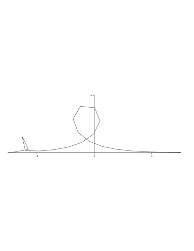
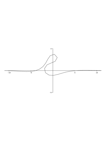
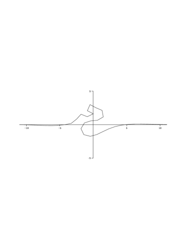
We present some pictures of the motions of the discrete curves. Figure 1 shows the simplest example of a curve, which corresponds to the 1-soliton solution (loop soliton).

Refer to caption
Figure 1: Parameters in equations (5.8), (5.9) and (5.10): N=1๐‘1N=1, x=0๐‘ฅ0x=0, y=0๐‘ฆ0y=0, ฮฑ1=โˆ’1subscript๐›ผ11\alpha_{1}=-1, ฮฒ1=โˆ’1subscript๐›ฝ11\beta_{1}=\sqrt{-1}, p1=0.3subscript๐‘10.3p_{1}=0.3, an=1subscript๐‘Ž๐‘›1a_{n}=1, bm=0.5subscript๐‘๐‘š0.5b_{m}=0.5.

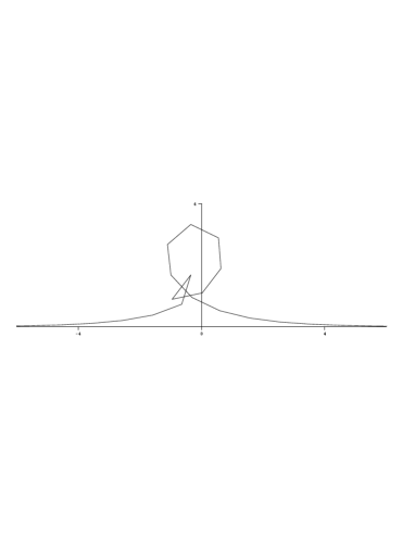
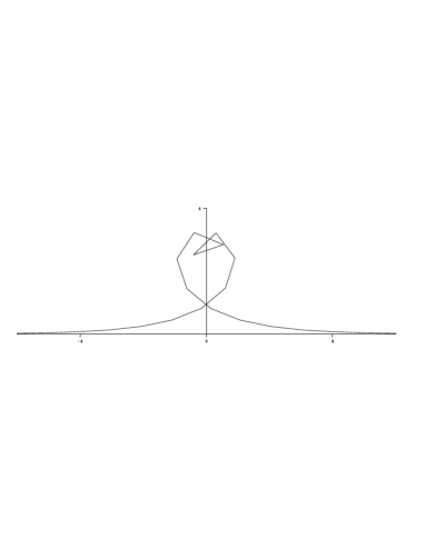
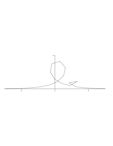
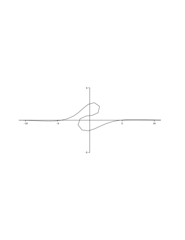
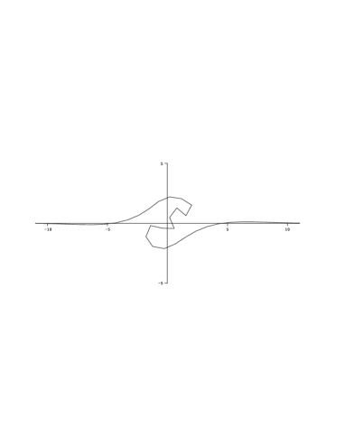
The next example illustrated in Figure 2 describes the interaction of two loops, which corresponds to the 2-soliton solution.

Refer to caption

m=โˆ’46๐‘š46m=-46

Refer to caption

m=โˆ’20๐‘š20m=-20

Refer to caption

m=โˆ’1๐‘š1m=-1

Refer to caption

m=30๐‘š30m=30

Figure 2: Parameters in equations (5.8), (5.9) and (5.10): N=2๐‘2N=2, x=0๐‘ฅ0x=0, y=0๐‘ฆ0y=0, ฮฑ1=โˆ’1subscript๐›ผ11\alpha_{1}=-1, ฮฑ2=1subscript๐›ผ21\alpha_{2}=1, ฮฒ1=โˆ’ฮฒ2=โˆ’1subscript๐›ฝ1subscript๐›ฝ21\beta_{1}=-\beta_{2}=\sqrt{-1}, p1=0.3subscript๐‘10.3p_{1}=0.3, p2=0.9subscript๐‘20.9p_{2}=0.9, an=1subscript๐‘Ž๐‘›1a_{n}=1, bm=0.5subscript๐‘๐‘š0.5b_{m}=0.5.

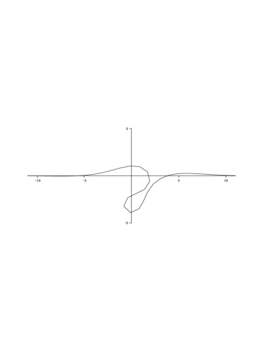
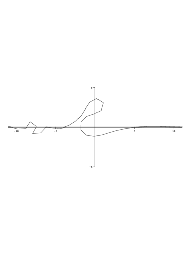
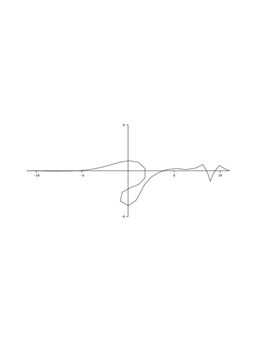
Figures 3 and 4 show the motions which correspond to the 1-breather and 2-breather solutions, respectively.

Refer to caption

m=โˆ’18๐‘š18m=-18

Refer to caption

m=โˆ’7๐‘š7m=-7

Refer to caption

m=โˆ’1๐‘š1m=-1

Refer to caption

m=20๐‘š20m=20

Figure 3: Parameters in equations (5.8), (5.9) and (5.10): N=2๐‘2N=2, x=0๐‘ฅ0x=0, y=0๐‘ฆ0y=0, ฮฑ1=ฮฑ2โˆ—=1subscript๐›ผ1superscriptsubscript๐›ผ21\alpha_{1}=\alpha_{2}^{*}=1, ฮฒ1=โˆ’ฮฒ2โˆ—=1subscript๐›ฝ1superscriptsubscript๐›ฝ21\beta_{1}=-\beta_{2}^{*}=1, p1=p2โˆ—=0.2โˆ’0.2โ€‹โˆ’1subscript๐‘1superscriptsubscript๐‘20.20.21p_{1}=p_{2}^{*}=0.2-0.2\sqrt{-1}, an=1subscript๐‘Ž๐‘›1a_{n}=1, bm=1.5subscript๐‘๐‘š1.5b_{m}=1.5.
Refer to caption

m=โˆ’18๐‘š18m=-18

Refer to caption

m=โˆ’7๐‘š7m=-7

Refer to caption

m=โˆ’1๐‘š1m=-1

Refer to caption

m=20๐‘š20m=20

Figure 4: Parameters in equations (5.8), (5.9) and (5.10): N=4๐‘4N=4, x=0๐‘ฅ0x=0, y=0๐‘ฆ0y=0, ฮฑ1=ฮฑ2โˆ—=1subscript๐›ผ1superscriptsubscript๐›ผ21\alpha_{1}=\alpha_{2}^{*}=1, ฮฑ3=ฮฑ4โˆ—=โˆ’1subscript๐›ผ3superscriptsubscript๐›ผ41\alpha_{3}=\alpha_{4}^{*}=\sqrt{-1}, ฮฒ1=โˆ’ฮฒ2โˆ—=1subscript๐›ฝ1superscriptsubscript๐›ฝ21\beta_{1}=-\beta_{2}^{*}=1, ฮฒ3=โˆ’ฮฒ4โˆ—=โˆ’1subscript๐›ฝ3superscriptsubscript๐›ฝ41\beta_{3}=-\beta_{4}^{*}=\sqrt{-1}, p1=p2โˆ—=0.2โˆ’0.2โ€‹โˆ’1subscript๐‘1superscriptsubscript๐‘20.20.21p_{1}=p_{2}^{*}=0.2-0.2\sqrt{-1}, p3=p4โˆ—=0.8+0.8โ€‹โˆ’1subscript๐‘3superscriptsubscript๐‘40.80.81p_{3}=p_{4}^{*}=0.8+0.8\sqrt{-1}, an=1subscript๐‘Ž๐‘›1a_{n}=1, bm=1.5subscript๐‘๐‘š1.5b_{m}=1.5.

5.2 Solutions via Bรคcklund transformations

In the theory of integrable systems, the Bรคcklund transformations are obtained from the shift of a certain discrete independent variable, which also applies to our geometric transformations. We first introduce discrete variables k๐‘˜k, l๐‘™l, and regard the determinant size N๐‘N as an additional discrete variable. We then extend the ฯ„๐œ\tau function as ฯ„nmโ€‹(k,l,N)=ฯ„nmโ€‹(x,t;y;k,l,N)superscriptsubscript๐œ๐‘›๐‘š๐‘˜๐‘™๐‘superscriptsubscript๐œ๐‘›๐‘š๐‘ฅ๐‘ก๐‘ฆ๐‘˜๐‘™๐‘\tau_{n}^{m}(k,l,N)=\tau_{n}^{m}(x,t;y;k,l,N) in the following way:

ฯ„nmโ€‹(k,l,N)=expโก[โˆ’(x+โˆ‘nโ€ฒnโˆ’1anโ€ฒ+โˆ‘mโ€ฒmโˆ’1bmโ€ฒ+โˆ‘kโ€ฒkโˆ’1ckโ€ฒ+โˆ‘lโ€ฒlโˆ’11dlโ€ฒ)โ€‹y]โ€‹det(fjโˆ’1(i))i,j=1,โ€ฆ,N,superscriptsubscript๐œ๐‘›๐‘š๐‘˜๐‘™๐‘๐‘ฅsuperscriptsubscriptsuperscript๐‘›โ€ฒ๐‘›1subscript๐‘Žsuperscript๐‘›โ€ฒsuperscriptsubscriptsuperscript๐‘šโ€ฒ๐‘š1subscript๐‘superscript๐‘šโ€ฒsuperscriptsubscriptsuperscript๐‘˜โ€ฒ๐‘˜1subscript๐‘superscript๐‘˜โ€ฒsuperscriptsubscriptsuperscript๐‘™โ€ฒ๐‘™11subscript๐‘‘superscript๐‘™โ€ฒ๐‘ฆsubscriptsuperscriptsubscript๐‘“๐‘—1๐‘–formulae-sequence๐‘–๐‘—1โ€ฆ๐‘\tau_{n}^{m}(k,l,N)=\exp\left[-\left(x+\sum_{n^{\prime}}^{n-1}a_{n^{\prime}}+\sum_{m^{\prime}}^{m-1}b_{m^{\prime}}+\sum_{k^{\prime}}^{k-1}c_{k^{\prime}}+\sum_{l^{\prime}}^{l-1}\frac{1}{d_{l^{\prime}}}\right)y\right]~{}\det\left(f_{j-1}^{(i)}\right)_{i,j=1,\ldots,N}, (5.21)
fs(i)=eฮทi+eฮผi,superscriptsubscript๐‘“๐‘ ๐‘–superscript๐‘’subscript๐œ‚๐‘–superscript๐‘’subscript๐œ‡๐‘–f_{s}^{(i)}=e^{\eta_{i}}+e^{\mu_{i}}, (5.22)
{eฮทi=ฮฑiโ€‹pisโ€‹โˆnโ€ฒnโˆ’1(1โˆ’anโ€ฒโ€‹pi)โˆ’1โ€‹โˆmโ€ฒmโˆ’1(1โˆ’bmโ€ฒโ€‹pi)โˆ’1โ€‹โˆkโ€ฒkโˆ’1(1โˆ’ckโ€ฒโ€‹pi)โˆ’1โ€‹โˆlโ€ฒlโˆ’1(1โˆ’dlโ€ฒpi)โˆ’1ร—epiโ€‹xโˆ’4โ€‹pi3โ€‹t+1piโ€‹y,eฮผj=ฮฒiโ€‹(โˆ’pi)sโ€‹โˆnโ€ฒnโˆ’1(1+anโ€ฒโ€‹pi)โˆ’1โ€‹โˆmโ€ฒmโˆ’1(1+bmโ€ฒโ€‹pi)โˆ’1โ€‹โˆkโ€ฒkโˆ’1(1+ckโ€ฒโ€‹pi)โˆ’1โ€‹โˆlโ€ฒlโˆ’1(1+dlโ€ฒpi)โˆ’1ร—eโˆ’piโ€‹x+4โ€‹pi3โ€‹tโˆ’1piโ€‹y.casessuperscript๐‘’subscript๐œ‚๐‘–subscript๐›ผ๐‘–superscriptsubscript๐‘๐‘–๐‘ superscriptsubscriptproductsuperscript๐‘›โ€ฒ๐‘›1superscript1subscript๐‘Žsuperscript๐‘›โ€ฒsubscript๐‘๐‘–1superscriptsubscriptproductsuperscript๐‘šโ€ฒ๐‘š1superscript1subscript๐‘superscript๐‘šโ€ฒsubscript๐‘๐‘–1superscriptsubscriptproductsuperscript๐‘˜โ€ฒ๐‘˜1superscript1subscript๐‘superscript๐‘˜โ€ฒsubscript๐‘๐‘–1superscriptsubscriptproductsuperscript๐‘™โ€ฒ๐‘™1superscript1subscript๐‘‘superscript๐‘™โ€ฒsubscript๐‘๐‘–1absentsuperscript๐‘’subscript๐‘๐‘–๐‘ฅ4superscriptsubscript๐‘๐‘–3๐‘ก1subscript๐‘๐‘–๐‘ฆsuperscript๐‘’subscript๐œ‡๐‘—subscript๐›ฝ๐‘–superscriptsubscript๐‘๐‘–๐‘ superscriptsubscriptproductsuperscript๐‘›โ€ฒ๐‘›1superscript1subscript๐‘Žsuperscript๐‘›โ€ฒsubscript๐‘๐‘–1superscriptsubscriptproductsuperscript๐‘šโ€ฒ๐‘š1superscript1subscript๐‘superscript๐‘šโ€ฒsubscript๐‘๐‘–1superscriptsubscriptproductsuperscript๐‘˜โ€ฒ๐‘˜1superscript1subscript๐‘superscript๐‘˜โ€ฒsubscript๐‘๐‘–1superscriptsubscriptproductsuperscript๐‘™โ€ฒ๐‘™1superscript1subscript๐‘‘superscript๐‘™โ€ฒsubscript๐‘๐‘–1absentsuperscript๐‘’subscript๐‘๐‘–๐‘ฅ4superscriptsubscript๐‘๐‘–3๐‘ก1subscript๐‘๐‘–๐‘ฆ\left\{\begin{array}[]{l}{\displaystyle e^{\eta_{i}}=\alpha_{i}p_{i}^{s}\prod_{n^{\prime}}^{n-1}(1-a_{n^{\prime}}p_{i})^{-1}\prod_{m^{\prime}}^{m-1}(1-b_{m^{\prime}}p_{i})^{-1}\prod_{k^{\prime}}^{k-1}(1-c_{k^{\prime}}p_{i})^{-1}\prod_{l^{\prime}}^{l-1}\left(1-\frac{d_{l^{\prime}}}{p_{i}}\right)^{-1}}\\ \hskip 100.0pt{\displaystyle\times~{}e^{p_{i}x-4p_{i}^{3}t+\frac{1}{p_{i}}y}},\\[11.38109pt] {\displaystyle e^{\mu_{j}}=\beta_{i}(-p_{i})^{s}\prod_{n^{\prime}}^{n-1}(1+a_{n^{\prime}}p_{i})^{-1}\prod_{m^{\prime}}^{m-1}(1+b_{m^{\prime}}p_{i})^{-1}\prod_{k^{\prime}}^{k-1}(1+c_{k^{\prime}}p_{i})^{-1}\prod_{l^{\prime}}^{l-1}\left(1+\frac{d_{l^{\prime}}}{p_{i}}\right)^{-1}}\\ \hskip 100.0pt{\displaystyle\times~{}e^{-p_{i}x+4p_{i}^{3}t-\frac{1}{p_{i}}y}}.\end{array}\right. (5.23)

Accordingly, we extend the relevant dependent variables such as ฮ˜ฮ˜\Theta and ฮณ๐›พ\gamma in the same way.

Proposition 5.2
  1. (1)1(\mathrm{1})

    For any kโˆˆโ„ค๐‘˜โ„คk\in\mathbb{Z}, ฮณ~โ€‹(x,t)=ฮณโ€‹(x,t;k+1)~๐›พ๐‘ฅ๐‘ก๐›พ๐‘ฅ๐‘ก๐‘˜1\widetilde{\gamma}(x,t)=\gamma(x,t;k+1) is a Bรคcklund transform of ฮณโ€‹(x,t)=ฮณโ€‹(x,t;k)๐›พ๐‘ฅ๐‘ก๐›พ๐‘ฅ๐‘ก๐‘˜\gamma(x,t)=\gamma(x,t;k) related by equation (4.3) with ฮป=1ck๐œ†1subscript๐‘๐‘˜\lambda=\frac{1}{c_{k}}.

  2. (2)2(\mathrm{2})

    For any kโˆˆโ„ค๐‘˜โ„คk\in\mathbb{Z}, ฮณ~nm=ฮณnmโ€‹(k+1)superscriptsubscript~๐›พ๐‘›๐‘šsuperscriptsubscript๐›พ๐‘›๐‘š๐‘˜1\widetilde{\gamma}_{n}^{m}=\gamma_{n}^{m}(k+1) is a Bรคcklund transform of ฮณnm=ฮณnmโ€‹(k)superscriptsubscript๐›พ๐‘›๐‘šsuperscriptsubscript๐›พ๐‘›๐‘š๐‘˜\gamma_{n}^{m}=\gamma_{n}^{m}(k) related by equation (4.16) with ฮป=1ck๐œ†1subscript๐‘๐‘˜\lambda=\frac{1}{c_{k}}.

  3. (3)3(\mathrm{3})

    For any Nโˆˆโ„คโ‰ฅ0๐‘subscriptโ„คabsent0N\in\mathbb{Z}_{\geq 0}, ฮณ~โ€‹(x,t)=ฮณโ€‹(x,t;N+1)~๐›พ๐‘ฅ๐‘ก๐›พ๐‘ฅ๐‘ก๐‘1\widetilde{\gamma}(x,t)=\gamma(x,t;N+1) is a Bรคcklund transform of ฮณโ€‹(x,t)=ฮณโ€‹(x,t;N)๐›พ๐‘ฅ๐‘ก๐›พ๐‘ฅ๐‘ก๐‘\gamma(x,t)=\gamma(x,t;N) related by equation (4.3) with ฮป=โˆ’pN+1๐œ†subscript๐‘๐‘1\lambda=-p_{N+1}.

  4. (4)4(\mathrm{4})

    For any Nโˆˆโ„คโ‰ฅ0๐‘subscriptโ„คabsent0N\in\mathbb{Z}_{\geq 0}, ฮณ~nm=ฮณnmโ€‹(N+1)superscriptsubscript~๐›พ๐‘›๐‘šsuperscriptsubscript๐›พ๐‘›๐‘š๐‘1\widetilde{\gamma}_{n}^{m}=\gamma_{n}^{m}(N+1) is a Bรคcklund transform of ฮณnm=ฮณnmโ€‹(N)superscriptsubscript๐›พ๐‘›๐‘šsuperscriptsubscript๐›พ๐‘›๐‘š๐‘\gamma_{n}^{m}=\gamma_{n}^{m}(N) related by equation (4.16) with ฮป=โˆ’pN+1๐œ†subscript๐‘๐‘1\lambda=-p_{N+1}.

  5. (5)5(\mathrm{5})

    For any lโˆˆโ„ค๐‘™โ„คl\in\mathbb{Z}, ฮณยฏโ€‹(x,t)=ฮณโ€‹(x,t;l+1)ยฏ๐›พ๐‘ฅ๐‘ก๐›พ๐‘ฅ๐‘ก๐‘™1\overline{\gamma}(x,t)=\gamma(x,t;l+1) is a Bรคcklund transform of ฮณโ€‹(x,t)=ฮณโ€‹(x,t;l)๐›พ๐‘ฅ๐‘ก๐›พ๐‘ฅ๐‘ก๐‘™\gamma(x,t)=\gamma(x,t;l) related by equation (4.21) with ฮป=dl๐œ†subscript๐‘‘๐‘™\lambda=d_{l}.

  6. (6)6(\mathrm{6})

    For any lโˆˆโ„ค๐‘™โ„คl\in\mathbb{Z}, ฮณยฏnm=ฮณnmโ€‹(l+1)superscriptsubscriptยฏ๐›พ๐‘›๐‘šsuperscriptsubscript๐›พ๐‘›๐‘š๐‘™1\overline{\gamma}_{n}^{m}=\gamma_{n}^{m}(l+1) is a Bรคcklund transform of ฮณnm=ฮณnmโ€‹(l)superscriptsubscript๐›พ๐‘›๐‘šsuperscriptsubscript๐›พ๐‘›๐‘š๐‘™\gamma_{n}^{m}=\gamma_{n}^{m}(l) related by equation (4.25) with ฮป=dl๐œ†subscript๐‘‘๐‘™\lambda=d_{l}.

Proof.โ€ƒWe first prove (1) and (2). It follows from equation (3.4) that the ฯ„๐œ\tau function satisfies the bilinear equation

Dyฯ„nm(k+1)โ‹…ฯ„nm(k)=โˆ’ckฯ„โˆ—(k+1)nmฯ„โˆ—(k)nm,D_{y}~{}\tau_{n}^{m}(k+1)\cdot\tau_{n}^{m}(k)=-c_{k}\tau^{*}{}_{n}^{m}(k+1)\tau^{*}{}_{n}^{m}(k), (5.24)

because of the symmetry with respect to the discrete variables m๐‘šm, n๐‘›n and k๐‘˜k in equations (5.21)โ€“(5.23). Then by an argument similar to that in the proof of Theorem 3.1, we see that

ฮณโ€‹(k+1)โˆ’ฮณโ€‹(k)ck=(cosโก(ฮธโ€‹(k+1)+ฮธโ€‹(k)2)sinโก(ฮธโ€‹(k+1)+ฮธโ€‹(k)2)).๐›พ๐‘˜1๐›พ๐‘˜subscript๐‘๐‘˜๐œƒ๐‘˜1๐œƒ๐‘˜2๐œƒ๐‘˜1๐œƒ๐‘˜2\frac{\gamma(k+1)-\gamma(k)}{c_{k}}=\left(\begin{array}[]{l}\vskip 6.0pt plus 2.0pt minus 2.0pt{\cos\left(\frac{\theta(k+1)+\theta(k)}{2}\right)}\\ {\sin\left(\frac{\theta(k+1)+\theta(k)}{2}\right)}\end{array}\right). (5.25)

From equation (2.4), we have equation (4.3) with ฮณ~=ฮณโ€‹(k+1)~๐›พ๐›พ๐‘˜1\widetilde{\gamma}=\gamma(k+1) and ฮธ~=ฮธโ€‹(k+1)~๐œƒ๐œƒ๐‘˜1\widetilde{\theta}=\theta(k+1):

ฮณโ€‹(k+1)โˆ’ฮณโ€‹(k)ck=Rโ€‹(ฮธโ€‹(k+1)โˆ’ฮธโ€‹(k)2)โ€‹ฮณโ€ฒโ€‹(k).๐›พ๐‘˜1๐›พ๐‘˜subscript๐‘๐‘˜๐‘…๐œƒ๐‘˜1๐œƒ๐‘˜2superscript๐›พโ€ฒ๐‘˜\frac{\gamma(k+1)-\gamma(k)}{c_{k}}=R\left(\frac{\theta(k+1)-\theta(k)}{2}\right)\gamma^{\prime}(k). (5.26)

Similarly from equation (3.16), we obtain equation (4.16) with ฮณ~nm=ฮณnmโ€‹(k+1)superscriptsubscript~๐›พ๐‘›๐‘šsuperscriptsubscript๐›พ๐‘›๐‘š๐‘˜1\widetilde{\gamma}_{n}^{m}=\gamma_{n}^{m}(k+1) and ฮ˜~nm=ฮ˜nmโ€‹(k+1)superscriptsubscript~ฮ˜๐‘›๐‘šsuperscriptsubscriptฮ˜๐‘›๐‘š๐‘˜1\widetilde{\Theta}_{n}^{m}=\Theta_{n}^{m}(k+1):

ฮณnmโ€‹(k+1)โˆ’ฮณnmโ€‹(k)ck=Rโ€‹(ฮ˜nmโ€‹(k+1)โˆ’ฮ˜n+1mโ€‹(k)2)โ€‹ฮณn+1mโ€‹(k)โˆ’ฮณnmโ€‹(k)an,superscriptsubscript๐›พ๐‘›๐‘š๐‘˜1superscriptsubscript๐›พ๐‘›๐‘š๐‘˜subscript๐‘๐‘˜๐‘…superscriptsubscriptฮ˜๐‘›๐‘š๐‘˜1superscriptsubscriptฮ˜๐‘›1๐‘š๐‘˜2superscriptsubscript๐›พ๐‘›1๐‘š๐‘˜superscriptsubscript๐›พ๐‘›๐‘š๐‘˜subscript๐‘Ž๐‘›\frac{\gamma_{n}^{m}(k+1)-\gamma_{n}^{m}(k)}{c_{k}}=R\left(\frac{\Theta_{n}^{m}(k+1)-\Theta_{n+1}^{m}(k)}{2}\right)\frac{\gamma_{n+1}^{m}(k)-\gamma_{n}^{m}(k)}{a_{n}}, (5.27)

which proves (1) and (2). The statements (3)โ€“(4) and (5)โ€“(6) can be proved in much the same way as (1)โ€“(2), by using the bilinear equations

Dyฯ„nm(N+1)โ‹…ฯ„nm(N)=1pN+1ฯ„โˆ—(N)nmฯ„โˆ—(N+1)nm,\displaystyle D_{y}~{}\tau_{n}^{m}(N+1)\cdot\tau_{n}^{m}(N)=\frac{1}{p_{N+1}}\tau^{*}{}_{n}^{m}(N)\tau^{*}{}_{n}^{m}(N+1), (5.28)
Dyฯ„nm(l+1)โ‹…ฯ„โˆ—(l)nm=โˆ’1dlฯ„โˆ—(l+1)nmฯ„nm(l),\displaystyle D_{y}~{}\tau_{n}^{m}(l+1)\cdot\tau^{*}{}_{n}^{m}(l)=-\frac{1}{d_{l}}\tau^{*}{}_{n}^{m}(l+1)\tau_{n}^{m}(l), (5.29)

respectively. These bilinear equations will be proved in Appendix. โ€ƒโ€ƒโ–กโ–ก\square

Remark 5.3

Here we give a physical interpretation of the Bรคcklund transformations described above. The Bรคcklund transforms in (1)โ€“(2) and (5)โ€“(6) of Proposition 5.2 correspond to changing the phase of solitons (loops), in other words, the positions of solitons. On the other hand, the Bรคcklund transforms in (3)โ€“(4) correspond to increasing the number of solitons (loops).

Computing the potential functions of the Bรคcklund transforms of the curves, one can verify the following result.

Corollary 5.4
  1. (1)1(\mathrm{1})

    For any kโˆˆโ„ค๐‘˜โ„คk\in\mathbb{Z}, ฮธ~โ€‹(x,t)=ฮธโ€‹(x,t;k+1)~๐œƒ๐‘ฅ๐‘ก๐œƒ๐‘ฅ๐‘ก๐‘˜1\widetilde{\theta}(x,t)=\theta(x,t;k+1) is a Bรคcklund transform of ฮธโ€‹(x,t)=ฮธโ€‹(x,t;k)๐œƒ๐‘ฅ๐‘ก๐œƒ๐‘ฅ๐‘ก๐‘˜\theta(x,t)=\theta(x,t;k) related by equations (2.5) and (2.6) with ฮป=1ck๐œ†1subscript๐‘๐‘˜\lambda=\frac{1}{c_{k}}.

  2. (2)2(\mathrm{2})

    For any kโˆˆโ„ค๐‘˜โ„คk\in\mathbb{Z}, ฮ˜~nm=ฮ˜nmโ€‹(k+1)superscriptsubscript~ฮ˜๐‘›๐‘šsuperscriptsubscriptฮ˜๐‘›๐‘š๐‘˜1\widetilde{\Theta}_{n}^{m}=\Theta_{n}^{m}(k+1) is a Bรคcklund transform of ฮ˜nm=ฮ˜nmโ€‹(k)superscriptsubscriptฮ˜๐‘›๐‘šsuperscriptsubscriptฮ˜๐‘›๐‘š๐‘˜\Theta_{n}^{m}=\Theta_{n}^{m}(k) related by equations (4.8) and (4.9) with ฮป=1ck๐œ†1subscript๐‘๐‘˜\lambda=\frac{1}{c_{k}}.

  3. (3)3(\mathrm{3})

    For any Nโˆˆโ„คโ‰ฅ0๐‘subscriptโ„คabsent0N\in\mathbb{Z}_{\geq 0}, ฮธ~โ€‹(x,t)=ฮธโ€‹(x,t;N+1)~๐œƒ๐‘ฅ๐‘ก๐œƒ๐‘ฅ๐‘ก๐‘1\widetilde{\theta}(x,t)=\theta(x,t;N+1) is a Bรคcklund transform of ฮธโ€‹(x,t)=ฮธโ€‹(x,t;N)๐œƒ๐‘ฅ๐‘ก๐œƒ๐‘ฅ๐‘ก๐‘\theta(x,t)=\theta(x,t;N) related by equations (2.5) and (2.6) with ฮป=โˆ’pN+1๐œ†subscript๐‘๐‘1\lambda=-p_{N+1}.

  4. (4)4(\mathrm{4})

    For any Nโˆˆโ„คโ‰ฅ0๐‘subscriptโ„คabsent0N\in\mathbb{Z}_{\geq 0}, ฮ˜~nm=ฮ˜nmโ€‹(N+1)superscriptsubscript~ฮ˜๐‘›๐‘šsuperscriptsubscriptฮ˜๐‘›๐‘š๐‘1\widetilde{\Theta}_{n}^{m}=\Theta_{n}^{m}(N+1) is a Bรคcklund transform of ฮ˜nm=ฮ˜nmโ€‹(N)superscriptsubscriptฮ˜๐‘›๐‘šsuperscriptsubscriptฮ˜๐‘›๐‘š๐‘\Theta_{n}^{m}=\Theta_{n}^{m}(N) related by equations (4.8) and (4.9) with ฮป=โˆ’pN+1๐œ†subscript๐‘๐‘1\lambda=-p_{N+1}.

  5. (5)5(\mathrm{5})

    For any lโˆˆโ„ค๐‘™โ„คl\in\mathbb{Z}, ฮธยฏโ€‹(x,t)=ฮธโ€‹(x,t;l+1)ยฏ๐œƒ๐‘ฅ๐‘ก๐œƒ๐‘ฅ๐‘ก๐‘™1\overline{\theta}(x,t)=\theta(x,t;l+1) is a Bรคcklund transform of ฮธโ€‹(x,t)=ฮธโ€‹(x,t;l)๐œƒ๐‘ฅ๐‘ก๐œƒ๐‘ฅ๐‘ก๐‘™\theta(x,t)=\theta(x,t;l) related by equations (4.19) and (4.20) with ฮป=dl๐œ†subscript๐‘‘๐‘™\lambda=d_{l}.

  6. (6)6(\mathrm{6})

    For any lโˆˆโ„ค๐‘™โ„คl\in\mathbb{Z}, ฮ˜ยฏ=nmฮ˜nm(l+1)\overline{\Theta}{}_{n}^{m}=\Theta_{n}^{m}(l+1) is a Bรคcklund transform of ฮ˜nm=ฮ˜nmโ€‹(l)superscriptsubscriptฮ˜๐‘›๐‘šsuperscriptsubscriptฮ˜๐‘›๐‘š๐‘™\Theta_{n}^{m}=\Theta_{n}^{m}(l) related by equations (4.23) and (4.24) with ฮป=dl๐œ†subscript๐‘‘๐‘™\lambda=d_{l}.

Appendix A Derivation of bilinear equations (5.28) and (5.29)

In this appendix, we show that the ฯ„๐œ\tau function given in equations (5.21)โ€“(5.23) actually satisfies the bilinear equations (5.28) and (5.29). For this purpose, we first introduce the generic ฯ„๐œ\tau function ฯ„nmโ€‹(k,l,N;s)=ฯ„nmโ€‹(x,t;y,z;k,l,N;s)superscriptsubscript๐œ๐‘›๐‘š๐‘˜๐‘™๐‘๐‘ superscriptsubscript๐œ๐‘›๐‘š๐‘ฅ๐‘ก๐‘ฆ๐‘ง๐‘˜๐‘™๐‘๐‘ \tau_{n}^{m}(k,l,N;s)=\tau_{n}^{m}(x,t;y,z;k,l,N;s) by

ฯ„nmโ€‹(k,l,N;s)=expโก[โˆ’(x+โˆ‘nโ€ฒnโˆ’1anโ€ฒ+โˆ‘mโ€ฒmโˆ’1bmโ€ฒ+โˆ‘kโ€ฒkโˆ’1ckโ€ฒ+โˆ‘lโ€ฒlโˆ’11dlโ€ฒ)โ€‹y]โ€‹det(fs+jโˆ’1(i))i,j=1,โ€ฆ,N,superscriptsubscript๐œ๐‘›๐‘š๐‘˜๐‘™๐‘๐‘ ๐‘ฅsuperscriptsubscriptsuperscript๐‘›โ€ฒ๐‘›1subscript๐‘Žsuperscript๐‘›โ€ฒsuperscriptsubscriptsuperscript๐‘šโ€ฒ๐‘š1subscript๐‘superscript๐‘šโ€ฒsuperscriptsubscriptsuperscript๐‘˜โ€ฒ๐‘˜1subscript๐‘superscript๐‘˜โ€ฒsuperscriptsubscriptsuperscript๐‘™โ€ฒ๐‘™11subscript๐‘‘superscript๐‘™โ€ฒ๐‘ฆsubscriptsuperscriptsubscript๐‘“๐‘ ๐‘—1๐‘–formulae-sequence๐‘–๐‘—1โ€ฆ๐‘\tau_{n}^{m}(k,l,N;s)=\exp\left[-\left(x+\sum_{n^{\prime}}^{n-1}a_{n^{\prime}}+\sum_{m^{\prime}}^{m-1}b_{m^{\prime}}+\sum_{k^{\prime}}^{k-1}c_{k^{\prime}}+\sum_{l^{\prime}}^{l-1}\frac{1}{d_{l^{\prime}}}\right)y\right]~{}\det\left(f_{s+j-1}^{(i)}\right)_{i,j=1,\ldots,N}, (A.1)

for (x,t;y,z)โˆˆโ„4๐‘ฅ๐‘ก๐‘ฆ๐‘งsuperscriptโ„4(x,t;y,z)\in\mathbb{R}^{4}, (m,n,k,l,s)โˆˆโ„ค5๐‘š๐‘›๐‘˜๐‘™๐‘ superscriptโ„ค5(m,n,k,l,s)\in\mathbb{Z}^{5} and Nโˆˆโ„คโ‰ฅ0๐‘subscriptโ„คabsent0N\in\mathbb{Z}_{\geq 0}. We require fs(i)=fs(i)โ€‹(x,t;y,z;m,n;k,l,N)superscriptsubscript๐‘“๐‘ ๐‘–superscriptsubscript๐‘“๐‘ ๐‘–๐‘ฅ๐‘ก๐‘ฆ๐‘ง๐‘š๐‘›๐‘˜๐‘™๐‘f_{s}^{(i)}=f_{s}^{(i)}(x,t;y,z;m,n;k,l,N) (i=1,โ€ฆ,N๐‘–1โ€ฆ๐‘i=1,\ldots,N) to satisfy the linear equations (5.2), (5.3) and

fs(i)โ€‹(k,l)โˆ’fs(i)โ€‹(kโˆ’1,l)ckโˆ’1=fs+1(i)โ€‹(k,l),fs(i)โ€‹(k,l)โˆ’fs(i)โ€‹(k,lโˆ’1)dlโˆ’1=fsโˆ’1(i)โ€‹(k,l).formulae-sequencesuperscriptsubscript๐‘“๐‘ ๐‘–๐‘˜๐‘™superscriptsubscript๐‘“๐‘ ๐‘–๐‘˜1๐‘™subscript๐‘๐‘˜1superscriptsubscript๐‘“๐‘ 1๐‘–๐‘˜๐‘™superscriptsubscript๐‘“๐‘ ๐‘–๐‘˜๐‘™superscriptsubscript๐‘“๐‘ ๐‘–๐‘˜๐‘™1subscript๐‘‘๐‘™1superscriptsubscript๐‘“๐‘ 1๐‘–๐‘˜๐‘™\frac{f_{s}^{(i)}(k,l)-f_{s}^{(i)}(k-1,l)}{c_{k-1}}=f_{s+1}^{(i)}(k,l),\quad\frac{f_{s}^{(i)}(k,l)-f_{s}^{(i)}(k,l-1)}{d_{l-1}}=f_{s-1}^{(i)}(k,l). (A.2)

A typical example for fs(i)superscriptsubscript๐‘“๐‘ ๐‘–f_{s}^{(i)} is given by

fs(i)=eฮทi+eฮผi,superscriptsubscript๐‘“๐‘ ๐‘–superscript๐‘’subscript๐œ‚๐‘–superscript๐‘’subscript๐œ‡๐‘–f_{s}^{(i)}=e^{\eta_{i}}+e^{\mu_{i}}, (A.3)
{eฮทi=ฮฑiโ€‹pisโ€‹โˆnโ€ฒnโˆ’1(1โˆ’anโ€ฒโ€‹pi)โˆ’1โ€‹โˆmโ€ฒmโˆ’1(1โˆ’bmโ€ฒโ€‹pi)โˆ’1โ€‹โˆkโ€ฒkโˆ’1(1โˆ’ckโ€ฒโ€‹pi)โˆ’1โ€‹โˆlโ€ฒlโˆ’1(1โˆ’dlโ€ฒpi)โˆ’1โ€‹epiโ€‹xโˆ’4โ€‹pi3โ€‹t+1piโ€‹y,eฮผj=ฮฒiโ€‹qisโ€‹โˆnโ€ฒnโˆ’1(1โˆ’anโ€ฒโ€‹qi)โˆ’1โ€‹โˆmโ€ฒmโˆ’1(1โˆ’bmโ€ฒโ€‹qi)โˆ’1โ€‹โˆkโ€ฒkโˆ’1(1โˆ’ckโ€ฒโ€‹qi)โˆ’1โ€‹โˆlโ€ฒlโˆ’1(1โˆ’dlโ€ฒqi)โˆ’1ร—eqiโ€‹xโˆ’4โ€‹qi3โ€‹t+1qiโ€‹y,casessuperscript๐‘’subscript๐œ‚๐‘–subscript๐›ผ๐‘–superscriptsubscript๐‘๐‘–๐‘ superscriptsubscriptproductsuperscript๐‘›โ€ฒ๐‘›1superscript1subscript๐‘Žsuperscript๐‘›โ€ฒsubscript๐‘๐‘–1superscriptsubscriptproductsuperscript๐‘šโ€ฒ๐‘š1superscript1subscript๐‘superscript๐‘šโ€ฒsubscript๐‘๐‘–1superscriptsubscriptproductsuperscript๐‘˜โ€ฒ๐‘˜1superscript1subscript๐‘superscript๐‘˜โ€ฒsubscript๐‘๐‘–1superscriptsubscriptproductsuperscript๐‘™โ€ฒ๐‘™1superscript1subscript๐‘‘superscript๐‘™โ€ฒsubscript๐‘๐‘–1superscript๐‘’subscript๐‘๐‘–๐‘ฅ4superscriptsubscript๐‘๐‘–3๐‘ก1subscript๐‘๐‘–๐‘ฆsuperscript๐‘’subscript๐œ‡๐‘—subscript๐›ฝ๐‘–superscriptsubscript๐‘ž๐‘–๐‘ superscriptsubscriptproductsuperscript๐‘›โ€ฒ๐‘›1superscript1subscript๐‘Žsuperscript๐‘›โ€ฒsubscript๐‘ž๐‘–1superscriptsubscriptproductsuperscript๐‘šโ€ฒ๐‘š1superscript1subscript๐‘superscript๐‘šโ€ฒsubscript๐‘ž๐‘–1superscriptsubscriptproductsuperscript๐‘˜โ€ฒ๐‘˜1superscript1subscript๐‘superscript๐‘˜โ€ฒsubscript๐‘ž๐‘–1superscriptsubscriptproductsuperscript๐‘™โ€ฒ๐‘™1superscript1subscript๐‘‘superscript๐‘™โ€ฒsubscript๐‘ž๐‘–1absentsuperscript๐‘’subscript๐‘ž๐‘–๐‘ฅ4superscriptsubscript๐‘ž๐‘–3๐‘ก1subscript๐‘ž๐‘–๐‘ฆ\left\{\begin{array}[]{l}{\displaystyle e^{\eta_{i}}=\alpha_{i}p_{i}^{s}\prod_{n^{\prime}}^{n-1}(1-a_{n^{\prime}}p_{i})^{-1}\prod_{m^{\prime}}^{m-1}(1-b_{m^{\prime}}p_{i})^{-1}\prod_{k^{\prime}}^{k-1}(1-c_{k^{\prime}}p_{i})^{-1}\prod_{l^{\prime}}^{l-1}\left(1-\frac{d_{l^{\prime}}}{p_{i}}\right)^{-1}e^{p_{i}x-4p_{i}^{3}t+\frac{1}{p_{i}}y}},\\[11.38109pt] {\displaystyle e^{\mu_{j}}=\beta_{i}q_{i}^{s}\prod_{n^{\prime}}^{n-1}(1-a_{n^{\prime}}q_{i})^{-1}\prod_{m^{\prime}}^{m-1}(1-b_{m^{\prime}}q_{i})^{-1}\prod_{k^{\prime}}^{k-1}(1-c_{k^{\prime}}q_{i})^{-1}\prod_{l^{\prime}}^{l-1}\left(1-\frac{d_{l^{\prime}}}{q_{i}}\right)^{-1}}\\ \hskip 100.0pt{\displaystyle\times~{}e^{q_{i}x-4q_{i}^{3}t+\frac{1}{q_{i}}y}},\end{array}\right. (A.4)

where pisubscript๐‘๐‘–p_{i}, qisubscript๐‘ž๐‘–q_{i}, ฮฑisubscript๐›ผ๐‘–\alpha_{i} and ฮฒisubscript๐›ฝ๐‘–\beta_{i} are arbitrary complex constants. We put

ฯƒnmโ€‹(y;k,l,N;s)=det(fs+jโˆ’1(i))i,j=1,โ€ฆ,N.superscriptsubscript๐œŽ๐‘›๐‘š๐‘ฆ๐‘˜๐‘™๐‘๐‘ subscriptsuperscriptsubscript๐‘“๐‘ ๐‘—1๐‘–formulae-sequence๐‘–๐‘—1โ€ฆ๐‘\sigma_{n}^{m}(y;k,l,N;s)=\det\left(f_{s+j-1}^{(i)}\right)_{i,j=1,\ldots,N}. (A.5)
Proposition A.1

The function ฯƒ๐œŽ\sigma satisfies the following bilinear equations:

Dyโ€‹ฯƒnmโ€‹(N+1;s)โ‹…ฯƒnmโ€‹(N;s)=ฯƒnmโ€‹(N;s+1)โ€‹ฯƒnmโ€‹(N+1;sโˆ’1),โ‹…subscript๐ท๐‘ฆsuperscriptsubscript๐œŽ๐‘›๐‘š๐‘1๐‘ superscriptsubscript๐œŽ๐‘›๐‘š๐‘๐‘ superscriptsubscript๐œŽ๐‘›๐‘š๐‘๐‘ 1superscriptsubscript๐œŽ๐‘›๐‘š๐‘1๐‘ 1\displaystyle D_{y}~{}\sigma_{n}^{m}(N+1;s)\cdot\sigma_{n}^{m}(N;s)=\sigma_{n}^{m}(N;s+1)\sigma_{n}^{m}(N+1;s-1), (A.6)
(Dyโˆ’1dl)โ€‹ฯƒnmโ€‹(l+1;s)โ‹…ฯƒnmโ€‹(l;s+1)=โˆ’1dlโ€‹ฯƒnmโ€‹(l+1;s+1)โ€‹ฯƒnmโ€‹(l;s).โ‹…subscript๐ท๐‘ฆ1subscript๐‘‘๐‘™superscriptsubscript๐œŽ๐‘›๐‘š๐‘™1๐‘ superscriptsubscript๐œŽ๐‘›๐‘š๐‘™๐‘ 11subscript๐‘‘๐‘™superscriptsubscript๐œŽ๐‘›๐‘š๐‘™1๐‘ 1superscriptsubscript๐œŽ๐‘›๐‘š๐‘™๐‘ \displaystyle\left(D_{y}-\frac{1}{d_{l}}\right)~{}\sigma_{n}^{m}(l+1;s)\cdot\sigma_{n}^{m}(l;s+1)=-\frac{1}{d_{l}}\sigma_{n}^{m}(l+1;s+1)\sigma_{n}^{m}(l;s). (A.7)

We apply the determinantal technique in order to prove Proposition A.1. The bilinear equations are reduced to the Plรผcker relations, which are quadratic identities of determinants whose columns are appropriately shifted. To this end, we construct such formulas that express the determinants in the Plรผcker relations in terms of the derivative or shift of a discrete variable of ฯƒnmโ€‹(k,l,N;s)superscriptsubscript๐œŽ๐‘›๐‘š๐‘˜๐‘™๐‘๐‘ \sigma_{n}^{m}(k,l,N;s) by using the linear relations of the entries. For the details of the technique, we refer to [22, 35, 34, 29, 30].

We introduce the notation

ฯƒnm(l,N;s)=|0l, 1l,โ‹ฏ,Nโˆ’2l,Nโˆ’1l|,\sigma_{n}^{m}(l,N;s)=\left|~{}0_{l},\ 1_{l},\ \cdots,\ N-2_{l},\ N-1_{l}~{}\right|, (A.8)

where โ€˜jlsubscript๐‘—๐‘™j_{l}โ€™ denotes the column vector

jl=[fs+j(1)โ€‹(l)โ‹ฎfs+j(N)โ€‹(l)].subscript๐‘—๐‘™delimited-[]superscriptsubscript๐‘“๐‘ ๐‘—1๐‘™โ‹ฎsuperscriptsubscript๐‘“๐‘ ๐‘—๐‘๐‘™j_{{l}}=\left[\begin{array}[]{c}f_{s+j}^{(1)}(l)\\ \vdots\\ f_{s+j}^{(N)}(l)\end{array}\right]. (A.9)
Lemma A.2

The following formulas hold:

โˆ‚yฯƒnm(l,N;s)=|โˆ’1, 1,โ‹ฏ,Nโˆ’2,Nโˆ’1|,\displaystyle\partial_{y}\sigma_{n}^{m}(l,N;s)=\left|~{}-1,\ 1,\ \cdots,\ N-2,\ N-1~{}\right|, (A.10)
ฯƒnm(l+1,N;s)=|0l+1, 1,โ‹ฏ,Nโˆ’2,Nโˆ’1|,\displaystyle\sigma_{n}^{m}(l+1,N;s)=\left|~{}0_{l+1},\ 1,\ \cdots,\ N-2,\ N-1~{}\right|, (A.11)
dlฯƒnm(l+1,N;s)=|1l+1, 1,โ‹ฏ,Nโˆ’2,Nโˆ’1|,\displaystyle d_{l}\sigma_{n}^{m}(l+1,N;s)=\left|~{}1_{l+1},\ 1,\ \cdots,\ N-2,\ N-1~{}\right|, (A.12)
โˆ’(dlโˆ‚yโˆ’1)ฯƒnm(l+1,N;s)=|0, 1l+1, 2,โ‹ฏ,Nโˆ’2,Nโˆ’1|.\displaystyle-\left(d_{l}\partial_{y}-1\right)\sigma_{n}^{m}(l+1,N;s)=\left|~{}0,\ 1_{l+1},\ 2,\ \cdots,\ N-2,\ N-1~{}\right|. (A.13)

Note that the subscripts of column vectors are shown only when l๐‘™l is shifted for notational simplicity.

Proof. Equation (A.10) can be verified by direct calculation by using the fourth equation in (5.2). We have

ฯƒnm(l+1,N;s)=|0l+1, 1l+1,โ‹ฏ,Nโˆ’2l+1,Nโˆ’1l+1|.\sigma_{n}^{m}(l+1,N;s)=\left|~{}0_{l+1},\ 1_{l+1},\ \cdots,\ N-2_{l+1},\ N-1_{l+1}~{}\right|. (A.14)

Adding the (Nโˆ’1)๐‘1(N-1)th column multiplied by dlsubscript๐‘‘๐‘™d_{l} to the N๐‘Nth column and using equation (A.2), we have

ฯƒnm(l+1,N;s)=|0l+1, 1l+1,โ‹ฏ,Nโˆ’2l+1,Nโˆ’1l|.\sigma_{n}^{m}(l+1,N;s)=\left|~{}0_{l+1},\ 1_{l+1},\ \cdots,\ N-2_{l+1},\ N-1_{l}~{}\right|. (A.15)

Similarly, adding the (iโˆ’1)๐‘–1(i-1)th column multiplied by dlsubscript๐‘‘๐‘™d_{l} to the i๐‘–ith column and using equation (A.2) for i=Nโˆ’1,โ€ฆ,2๐‘–๐‘1โ€ฆ2i=N-1,\ldots,2, we obtain

ฯƒnm(l+1,N;s)=|0l+1, 1,โ‹ฏ,Nโˆ’2,Nโˆ’1|,\sigma_{n}^{m}(l+1,N;s)=\left|~{}0_{l+1},\ 1,\ \cdots,\ N-2,\ N-1~{}\right|, (A.16)

which is equation (A.11). Multiplying dlsubscript๐‘‘๐‘™d_{l} to the first column of equation (A.11) and using equation (A.2), we obtain equation (A.12). Finally, differentiating equation (A.12) with respect to y๐‘ฆy yields

dlโ€‹โˆ‚yฯƒnmโ€‹(l+1,N;s)subscript๐‘‘๐‘™subscript๐‘ฆsuperscriptsubscript๐œŽ๐‘›๐‘š๐‘™1๐‘๐‘ \displaystyle d_{l}\partial_{y}\sigma_{n}^{m}(l+1,N;s) =|0l+1, 1, 2,โ‹ฏ,Nโˆ’2,Nโˆ’1|+|1l+1, 0, 2,โ‹ฏ,Nโˆ’2,Nโˆ’1|\displaystyle=\left|~{}0_{l+1},\ 1,\ 2,\ \cdots,\ N-2,\ N-1~{}\right|+\left|~{}1_{l+1},\ 0,\ 2,\ \cdots,\ N-2,\ N-1~{}\right|
=ฯƒnm(l+1,N;s)โˆ’|0, 1l+1, 2,โ‹ฏ,Nโˆ’2,Nโˆ’1|,\displaystyle=\sigma_{n}^{m}(l+1,N;s)-\left|~{}0,\ 1_{l+1},\ 2,\ \cdots,\ N-2,\ N-1~{}\right|, (A.17)

which is equivalent to equation (A.13). This completes the proof. โ€ƒโ€ƒโ–กโ–ก\square


Proof of Proposition A.1โ€ƒConsider the Plรผcker relation (see, for example, [35]),

0=|โˆ’1,0,1,โ‹ฏ,Nโˆ’2|ร—|1,โ‹ฏ,Nโˆ’2,Nโˆ’1,ฯ•|+|0,1,โ‹ฏ,Nโˆ’2,Nโˆ’1|ร—|โˆ’1,1,โ‹ฏ,Nโˆ’2,ฯ•|โˆ’|0,1,โ‹ฏ,Nโˆ’2,ฯ•|ร—|โˆ’1,1,โ‹ฏ,Nโˆ’2,Nโˆ’1|,\begin{split}0=&\left|~{}-1,0,1,\cdots,N-2~{}\right|\times\left|~{}1,\cdots,N-2,N-1,\phi~{}\right|\\ +&\left|~{}0,1,\cdots,N-2,N-1~{}\right|\times\left|~{}-1,1,\cdots,N-2,\phi~{}\right|\\ -&\left|~{}0,1,\cdots,N-2,\phi~{}\right|\times\left|~{}-1,1,\cdots,N-2,N-1~{}\right|,\end{split} (A.18)

where ฯ•italic-ฯ•\phi is a column vector given by

ฯ•=[0โ‹ฎ01].italic-ฯ•delimited-[]0โ‹ฎ01\phi=\left[\begin{array}[]{c}0\\ \vdots\\ 0\\ 1\end{array}\right]. (A.19)

By using equations (A.8) and (A.10), expanding the determinant with respect to the column ฯ•italic-ฯ•\phi, equation (A.18) can be rewritten as

0=ฯƒnmโ€‹(N;sโˆ’1)โ€‹ฯƒnmโ€‹(Nโˆ’1;s+1)+ฯƒnmโ€‹(N;s)โ€‹โˆ‚yฯƒnmโ€‹(Nโˆ’1;s)โˆ’ฯƒnmโ€‹(Nโˆ’1;s)โ€‹โˆ‚yฯƒnmโ€‹(N;s),0superscriptsubscript๐œŽ๐‘›๐‘š๐‘๐‘ 1superscriptsubscript๐œŽ๐‘›๐‘š๐‘1๐‘ 1superscriptsubscript๐œŽ๐‘›๐‘š๐‘๐‘ subscript๐‘ฆsuperscriptsubscript๐œŽ๐‘›๐‘š๐‘1๐‘ superscriptsubscript๐œŽ๐‘›๐‘š๐‘1๐‘ subscript๐‘ฆsuperscriptsubscript๐œŽ๐‘›๐‘š๐‘๐‘ 0=\sigma_{n}^{m}(N;s-1)~{}\sigma_{n}^{m}(N-1;s+1)+\sigma_{n}^{m}(N;s)~{}\partial_{y}\sigma_{n}^{m}(N-1;s)-\sigma_{n}^{m}(N-1;s)~{}\partial_{y}\sigma_{n}^{m}(N;s), (A.20)

which implies equation (A.6). Similarly, applying Lemma A.2 on the Plรผcker relation

0=|โˆ’1,0,1,โ‹ฏ,Nโˆ’2|ร—|0l+1,1,โ‹ฏ,Nโˆ’2,Nโˆ’1|โˆ’|0l+1,0,1,โ‹ฏ,Nโˆ’2|ร—|โˆ’1,1,โ‹ฏ,Nโˆ’2,Nโˆ’1|โˆ’|0,1,โ‹ฏ,Nโˆ’2,Nโˆ’1|ร—|โˆ’1,0l+1,1,โ‹ฏ,Nโˆ’2|,\begin{split}0=&\left|~{}-1,0,1,\cdots,N-2~{}\right|\times\left|~{}0_{l+1},1,\cdots,N-2,N-1~{}\right|\\ -&\left|~{}0_{l+1},0,1,\cdots,N-2~{}\right|\times\left|~{}-1,1,\cdots,N-2,N-1~{}\right|\\ -&\left|~{}0,1,\cdots,N-2,N-1~{}\right|\times\left|~{}-1,0_{l+1},1,\cdots,N-2~{}\right|,\end{split} (A.21)

we obtain

0=ฯƒnmโ€‹(l;sโˆ’1)ร—ฯƒnmโ€‹(l+1;s)โˆ’dlโ€‹ฯƒnmโ€‹(l+1;sโˆ’1)ร—โˆ‚yฯƒnmโ€‹(l;s)โˆ’ฯƒnmโ€‹(l;s)ร—[โˆ’(dlโ€‹โˆ‚yโˆ’1)โ€‹ฯƒnmโ€‹(l+1;sโˆ’1)],0superscriptsubscript๐œŽ๐‘›๐‘š๐‘™๐‘ 1superscriptsubscript๐œŽ๐‘›๐‘š๐‘™1๐‘ subscript๐‘‘๐‘™superscriptsubscript๐œŽ๐‘›๐‘š๐‘™1๐‘ 1subscript๐‘ฆsuperscriptsubscript๐œŽ๐‘›๐‘š๐‘™๐‘ superscriptsubscript๐œŽ๐‘›๐‘š๐‘™๐‘ delimited-[]subscript๐‘‘๐‘™subscript๐‘ฆ1superscriptsubscript๐œŽ๐‘›๐‘š๐‘™1๐‘ 1\begin{split}0&=\sigma_{n}^{m}(l;s-1)\times\sigma_{n}^{m}(l+1;s)-d_{l}\sigma_{n}^{m}(l+1;s-1)\times\partial_{y}\sigma_{n}^{m}(l;s)\\ &-\sigma_{n}^{m}(l;s)\times\left[-(d_{l}\partial_{y}-1)\sigma_{n}^{m}(l+1;s-1)\right],\end{split} (A.22)

which is equivalent to equation (A.7). This completes the proof. โ€ƒโ€ƒโ–กโ–ก\square


From Proposition A.1 and equation (A.1), we see that ฯ„nmโ€‹(k,l,N;s)superscriptsubscript๐œ๐‘›๐‘š๐‘˜๐‘™๐‘๐‘ \tau_{n}^{m}(k,l,N;s) satisfies

Dyโ€‹ฯ„nmโ€‹(N+1;s)โ‹…ฯ„nmโ€‹(N;s)=ฯ„nmโ€‹(N;s+1)โ€‹ฯ„nmโ€‹(N+1;sโˆ’1),โ‹…subscript๐ท๐‘ฆsuperscriptsubscript๐œ๐‘›๐‘š๐‘1๐‘ superscriptsubscript๐œ๐‘›๐‘š๐‘๐‘ superscriptsubscript๐œ๐‘›๐‘š๐‘๐‘ 1superscriptsubscript๐œ๐‘›๐‘š๐‘1๐‘ 1\displaystyle D_{y}~{}\tau_{n}^{m}(N+1;s)\cdot\tau_{n}^{m}(N;s)=\tau_{n}^{m}(N;s+1)\tau_{n}^{m}(N+1;s-1), (A.23)
Dyโ€‹ฯ„nmโ€‹(l+1;s)โ‹…ฯ„nmโ€‹(l;s+1)=โˆ’1dlโ€‹ฯ„nmโ€‹(l+1;s+1)โ€‹ฯ„nmโ€‹(l;s).โ‹…subscript๐ท๐‘ฆsuperscriptsubscript๐œ๐‘›๐‘š๐‘™1๐‘ superscriptsubscript๐œ๐‘›๐‘š๐‘™๐‘ 11subscript๐‘‘๐‘™superscriptsubscript๐œ๐‘›๐‘š๐‘™1๐‘ 1superscriptsubscript๐œ๐‘›๐‘š๐‘™๐‘ \displaystyle D_{y}~{}\tau_{n}^{m}(l+1;s)\cdot\tau_{n}^{m}(l;s+1)=-\frac{1}{d_{l}}\tau_{n}^{m}(l+1;s+1)\tau_{n}^{m}(l;s). (A.24)

We finally obtain equations (5.28) and (5.29) from equations (A.23) and (A.24), respectively, by imposing the reduction condition (3.30).
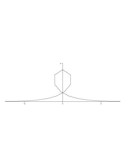
Acknowledgements

One of the authors (K.K.) would like to thank Professor Tim Hoffmann for giving a series of introductory lectures on discrete differential geometry at Kyushu University. This work is partially supported by JSPS Grant-in-Aid for Scientific Research No.ย 19340039, 21540067, 21656027 and 22656026.

References

  • [1] M. J. Ablowitz B. Prinari and A.D. Trubatch, Discrete and Continuous Nonlinear Schrรถdinger Systems (Cambridge University Press, Cambridge, 2004).
  • [2] L. Bianchi, Sulla trasformazione di Bรคcklund per le superficie pseudosferiche, Rend. Lincei 5(1892) 3โ€“12.
  • [3] A. Bobenko and U. Pinkall, Discrete surface with constant negative Gaussian curvature and the Hirota equation, J. Differential Geom. 43(1996) 527โ€“611.
  • [4] A.I. Bobenko and Y.B. Suris, Discrete Differential Geometry (American Mathematical Society, Prividence, RI, 2008).
  • [5] E. Date, M. Jimbo and T. Miwa, Method for generating discrete soliton equations.I, J. Phys. Soc. Jpn. 51(1982) 4116โ€“4124.
  • [6] E. Date, M. Jimbo and T. Miwa, Method for generating discrete soliton equations.II, J. Phys. Soc. Jpn. 51(1982) 4125โ€“4131.
  • [7] E. Date, M. Jimbo and T. Miwa, Method for generating discrete soliton equations.III, J. Phys. Soc. Jpn. 52(1983) 388โ€“393.
  • [8] E. Date, M. Jimbo and T. Miwa, Method for generating discrete soliton equations.IV, J. Phys. Soc. Jpn. 52(1983) 761โ€“765.
  • [9] E. Date, M. Jimbo and T. Miwa, Method for generating discrete soliton equations.V, J. Phys. Soc. Jpn. 52(1983) 766โ€“771.
  • [10] A. Doliwa, Geometric discretization of the Toda system, Phys. Lett. A234(1997)187โ€“192.
  • [11] A. Doliwa and P.M. Santini, Integrable dynamics of a discrete curve and the Ablowitz-Ladik hierarchy, J. Math. Phys. 36 (1995)1259โ€“1273.
  • [12] A. Doliwa and P.M. Santini, The integrable dynamic of a discrete curve, Symmetries and Integrability of Difference Equations, D. Levi, L. Vinet and P. Winternitz (eds.), (AMS, Providence 1996) 91โ€“102.
  • [13] A. Doliwa and P.M. Santini, Geometry of discrete curves and lattices and integrable difference equations, Discrete Integrable Geometry and Physics, A. Bobenko and R. Seiler (eds.), (Clarendon Press, Oxford, 1999) 139โ€“154.
  • [14] R.ย E.ย Goldstein and D.ย M.ย Petrich, The Korteweg-de Vries hierarchy as dynamics of closed curves in the plane, Phys. Rev. Lett. 67 (1991) 3203โ€“3206.
  • [15] H. Hasimoto, A soliton on a vortex filament, J. Fluid. Mech. 11(1972) 477โ€“485.
  • [16] R. Hirota, Nonlinear partial difference equations. I. A difference analogue of the Korteweg-de Vries equation, J. Phys. Soc. Jpn. 43(1977) 1429โ€“1433.
  • [17] R. Hirota, Nonlinear partial difference equations. II. Discrete-time Toda equation, J. Phys. Soc. Jpn. 43(1977) 2074โ€“2078.
  • [18] R. Hirota, Nonlinear partial difference equations. III. Discrete sine-Gordon equation, J. Phys. Soc. Jpn. 43(1977) 2079โ€“2086.
  • [19] R. Hirota, Nonlinear partial difference equations. IV. Bรคcklund transformation for the discrete-time Toda equation, J. Phys. Soc. Jpn. 45(1978) 321โ€“332.
  • [20] R. Hirota, Nonlinear partial difference equations. V. Nonlinear equations reducible to linear equations, J. Phys. Soc. Jpn. 46(1979) 312โ€“319.
  • [21] R. Hirota, Discretization of the potential modified KdV equation, J. Phys. Soc. Jpn. 67(1998) 2234โ€“2236.
  • [22] R. Hirota, The Direct Method in Soliton Theory, Cambridge Tracts in Mathematics 155 (Cambridge University Press, Cambridge, 2004)
  • [23] M.ย Hisakado, K.ย Nakayama and M.ย Wadati, Motion of discrete curves in the plane, J. Phys. Soc. Jpn. 64 (1995) 2390โ€“2393.
  • [24] T.Hoffmann, Discrete Hashimoto surfaces and a doubly discrete smoke-ring flow, Discrete Differential Geometry, A.I. Bobenko, P. Schrรถder, J.M. Sullivan and G.M. Ziegler (eds.), Oberwolfach Seminars Vol.39 (Birkhรคuser, Basel, 2008)95โ€“115.
  • [25] T. Hoffmann, Discrete Differential Geometry of Curves and Surfaces, COE lecture Notes Vol. 18 (Kyushu University, Fukuoka, 2009).
  • [26] T.ย Hoffmann and N.ย Kutz, Discrete curves in โ„‚โ€‹P1โ„‚superscript๐‘ƒ1\mathbb{C}P^{1} and the Toda lattice, Stud. Appl. Math. 113 (2004) 31โ€“55.
  • [27] M. Jimbo and T. Miwa, Solitons and infinite dimensional Lie algebras, Publ. RIMS 19(1983) 943-1001.
  • [28] G.ย Lamb Jr., Solitons and the motion of helical curves, Phys. Rev. Lett. 37 (1976) 235โ€“237.
  • [29] K. Maruno, K. Kajiwara and M. Oikawa, Casorati determinant solution for the discrete-time relativistic Toda lattice equation, Phys. Lett. A241(1998) 335โ€“343.
  • [30] K. Maruno and Y. Ohta, Casorati determinant form of dark soliton solutions of the discrete nonlinear Schrรถdinger equation, J. Phys. Soc. Jpn. 75(2006) 054002.
  • [31] N.ย Matsuura, Discrete KdV and discrete modified KdV equations arising from motions of discrete planar curves, Int. Math. Res. Not. IMRN Advance Access published May 15, 2011, doi:10.1093/imrn/rnr080.
  • [32] T. Miwa, On Hirotaโ€™s difference equations, Proc. Japan Acad. Ser. A Math. Sci. 58(1982) 9โ€“12.
  • [33] F.W. Nijhoff and H. Capel, The discrete KdV equation, Acta Appl. Math. 39(1995) 133โ€“158.
  • [34] Y. Ohta, R. Hirota, S. Tsujimoto and T. Imai, Casorati and discrete Gram type determinant representations of solutions to the discrete KP hierarchy, J. Phys. Soc. Jpn. 62(1993) 1872โ€“1886.
  • [35] Y. Ohta, K. Kajiwara, J. Matsukidaira and J. Satsuma, Casorati determinant solution for the relativistic Toda lattice equation, J. Math. Phys. 34(1993) 5190โ€“5204.
  • [36] U. Pinkall, B. Springborn, and S. WeiรŸmann, A new doubly discrete analogue of smoke ring flow and the real time simulation of fluid flow, J. Phys. A: Math. Theor. 40 (2007) 1256312576.
  • [37] C. Rogers and W.K. Schief, Bรคcklund and Darboux Transformations: Geometry and Modern Applications in Soliton Theory, Cambridge Texts in Applied Mathematics (Cambridge University Press, Cambridge, 2002).
  • [38] Y. B. Suris, The Problem of Integrable Discretization (Birkhรคuser, Basel, 2003).
  • [39] S. Tsujimoto, On a discrete analogue of the two-dimensional Toda lattice hierarchy, Publ. RIMS 38(2002) 113-133.
  • [40] K. Ueno and K. Takasaki, Toda lattice hierarchy, Group Representations and Systems of Differential Equations, Adv. Stud. Pure Math. 4 (Kinokuniya, Tokyo, 1982) 1โ€“95.
  • [41] M. Wadati, Bรคcklund transformation for solutions of the modified Korteweg-de Vries equation, J. Phys. Soc. Jpn. 36(1974) 1498.