Current characteristics of mesoscopic rings in quantum Smoluchowski regime

Abstract

In normal mesoscopic metals of a ring topology persistent currents can be induced by threading the center of the ring with a magnetic flux. This phenomenon is an example of the famous Aharonov-Bohm effect. In the paper we study the current vs the external constant magnetic flux characteristics of the system driven by both the classical and the quantum thermal fluctuations. The problem is formulated in terms of Langevin equations in classical and quantum Smoluchowski regimes. We analyze the impact of the quantum thermal fluctuations on the current-flux characteristics. We demonstrate that the current response can be changed from paramagnetic to diamagnetic when the quantum nature of the thermal fluctuations increases.

1 Introduction

Mesoscopic systems lay at the border between macroscopic and microscopic worlds. Mesoscopic systems, consisting of a large number of atoms, are too big to study their properties by the quantum methods of individual atoms, and are too small to apply physical laws of the macro-world. For their description and modeling one should combine both methods appreciating and recognizing the role of quantum and classical processes. The appearance of a new length scale - the phase coherence length $l_{c}$ of electronic wave functions - introduces various regimes for transport phenomena influenced by quantum interference effects. The mesoscopic regime is characterized by small length scales and low temperatures. When the temperature is lowered, the phase coherence length increases and the mesoscopic regime is extended to larger length scales. At sub-Kelvin temperatures, the length scales are of the order of micrometers. The most prominent mesoscopic effects are: the Aharonov-Bohm oscillations in the conductance of mesoscopic structures, the quantum Hall effects, the universal conductance fluctuations and persistent currents in mesoscopic normal metal rings threaded by a magnetic flux. Persistent currents have been known to exist in superconductors in which they are related to the existence of a state with zero resistance and the fact that a superconductor is a perfect diamagnet. The existence of persistent currents in normal (i.e. non-superconducting) metals is, in fact, a manifestation of the famous Aharonov-Bohm effect. Persistent currents have been predicted by Hund in 1938 hund and re-discovered later by others but . Inspired by these findings, the first experiment was performed in the early 1990s by measuring the magnetization of an array of about ten million not connected micron-sized copper rings buh . Other experiments also supported existence of persistent currents chandra . We should also recall recent definitive measurements of persistent currents in nanoscale gold and aluminium rings harris ; bluhm . The team harris has developed a new technique for detecting persistent currents that allows to measure the persistent current over a wide range of temperatures, ring sizes, and magnetic fields. They have used nanoscale cantilevers, an entirely novel approach to indirectly measure the current through changes in the magnetic force it produces as it flows through the ring. The second team bluhm has studied thirty three individual rings, in which they have employed a scanning technique (a SQUID microscope). The rings are very small, each only between one and two micrometers in diameter and 140 nanometers thick. They are made of high-purity gold. Each was scanned individually, unlike past experiments on persistent currents conducted by other groups. In total they were scanned approximately 10 million times. Both works mark the first time that the theory has been experimentally proven to a high degree.

In our previous papers rogo we have proposed a two-fluid model for the dynamics of the magnetic flux that passes through a mesoscopic ring. It is described in terms of an ordinary differential equation with an additional random force. It is analogous to the well known model of a capacitively and a resistively shunted Josephson junction barone . The classical part consists of ’normal’ electrons carrying dissipative current. The quantum part is formed by those electrons which maintain their phase coherence around the circumference of the ring (it is a counterpart of the Cooper pairs of the electrons in the superconducting systems). The effective dynamics is than determined by a classical Langevin equation lutz with a Johnson noise describing classical thermal equilibrium fluctuations. For low temperatures, quantum nature of thermal fluctuations should be taken into account. To this aim we apply the approach based on the so called quantum Smoluchowski equation as introduced in Ref. ankerhold1 and in other versions in the following Refs. luczka ; ankerhold2 ; coffey .

The paper is organized as follows. First, in the Sec. 2, we present a model of capacitively and resistively shunted Josephson junction in order to demonstrate readers the analogy between both models. Next, in the Sec. 3, we briefly present our model for the flux dynamics in the normal metal rings. In the Sec. 4, we define the quantum Smoluchowski regime following by the Sec. 5, presenting the dimensionless variables and parameters. In the Sec. 6, we study the current characteristics in the stationary states for both classical and quantum Smoluchowski domain. We end this work with the summary and conclusions.

2 Superconducting ring

For clarity of modeling the current characteristics in non-superconducting rings, we present the well-known approach to describe a quasi-classical regime of superconducting rings. To this aim, let us consider a superconducting loop (ring, cylinder, torus) interrupted by a Josephson junction. This element is a basic unit of various SQUID devices. The phase difference $\psi$ of the Cooper pair wave function across the junction is related to the magnetic flux $\phi$ threading the ring via the relation barone

$$\psi=2\pi(n-\phi/\phi_{0}),$$ (1)

where $2\pi n$ is the phase change per cycle around the ring and $\phi_{0}=h/2e$ is the flux quantum. When the external magnetic field is applied, the total flux is

$$\phi=\phi_{e}+LI,$$ (2)

where $\phi_{e}$ is the flux generated by an applied external magnetic field, $L$ is the self-inductance of the ring and $I$ is the total current flowing in the ring. We model the Josephson element in terms of the resistively and capacitively shunted junction for which the current consists of three components kos , namely,

$$I=I_{C}+I_{R}+I_{J}=\frac{\phi-\phi_{e}}{L},$$ (3)

where $I_{C}$ is a displacement current accompanied with the junction capacitance $C$, $I_{R}$ is a normal (Ohmic) current characterized by the normal state resistance $R$ and $I_{J}$ is the Josephson supercurrent. In the right-hand side, the relation (2) has beed used.

Combining Eqs. (1)-(3) with the second Josephson relation $d\psi/dt=2eU/\hbar$, where $U$ is the voltage drop across the junction, we get the Langevin-type equation in the form barone

$$C\frac{d^{2}\phi}{dt^{2}}+\frac{1}{R}\frac{d\phi}{dt}+I_{0}\sin\phi=-\frac{\phi-\phi_{e}}{L}+\sqrt{\frac{2k_{B}T}{R}}\Gamma(t).$$ (4)

This equation has a mechanical interpretation: it can describe the ’position’ $\phi(t)$ of the Brownian particle moving in the washboard potential

$$W(\phi)=\frac{(\phi-\phi_{e})^{2}}{2L}-I_{0}\cos\phi.$$ (5)

The first term originates from the external bias and the self–inductive interaction of the magnetic flux whereas the second term is the supercurrent modified by the quantum flux. The ubiquitous thermal equilibrium noise $\Gamma(t)$ consists of Johnson noise associated with the resistance $R$. The parameter $k_{B}$ denotes the Boltzmann constant and $T$ is temperature of the system. The Johnson noise is modeled by $\delta$-correlated Gaussian white noise of zero mean, $\langle\Gamma(t)\rangle=0$, and unit intensity, i.e., $\langle\Gamma(t)\Gamma(u)\rangle=\delta(t-u)$.

3 Normal metal ring

Now, let us consider a non-superconducting ring. When the external magnetic field is applied, the actual flux is given by

$$\phi=\phi_{e}+LI,$$ (6)

where $\phi_{e}$ is the flux generated by an applied external magnetic field, $L$ is the self-inductance of the ring and $I$ is the total current flowing in the ring. At zero temperature, the ring displays persistent and non-dissipative currents $I_{P}$ run by phase-coherent electrons. It is analogue of the Josephson supercurrent $I_{J}$. At non-zero temperature, a part of electrons becomes ’normal’ (non-coherent) and the amplitude of the persistent current decreases. Moreover, resistance of the ring and thermal fluctuations should be taken into account. Therefore for temperatures $T>0$, the total current consists of three parts, namely,

$$I=I_{C}+I_{R}+I_{P}=\frac{\phi-\phi_{e}}{L}.$$ (7)

What we need is the expression for the persistent current $I_{P}$. It is s function of the magnetic flux $\phi$ and depends on the parity of the number of coherent electrons. Let $p$ denotes the probability of an even number of coherent electrons and $1-p$ is the probability of an odd number of coherent electrons. Then the persistent current can be expressed in the form cheng

$$I_{P}=I_{P}(\phi)=p\,I_{E}(\phi)+(1-p)\,I_{O}(\phi),$$ (8)

where

$$I_{E}(\phi)=I_{O}(\phi+\phi_{0}/2)=I_{0}\sum_{n=1}^{\infty}A_{n}(T/T^{*})\cos(nk_{F}l)\sin(2n\pi\phi/\phi_{0}),$$ (9)

where $I_{0}$ is the maximal current at zero temperature. The temperature dependent amplitudes are determined by the relation cheng

$$A_{n}(T/T^{*})=\frac{4T}{\pi T^{*}}\frac{\exp(-nT/T^{*})}{1-\exp(-2nT/T^{*})},$$ (10)

where the characteristic temperature $T^{*}$ is proportional to the energy gap $\Delta_{F}$ at the Fermi surface, $k_{F}$ is the Fermi momentum and $l$ is the circumference of the ring. If the number $N$ of electrons is fixed then $k_{F}=\pi N/l$ and the persistent current takes the form

$$I_{P}(\phi)=I_{0}\sum_{n=1}^{\infty}A_{n}(T/T^{*})\sin(2n\pi\phi/\phi_{0})[p+(-1)^{n}(1-p)].$$ (11)

As a result, from Eq. (7) we obtain the equation of motion in the form rogo

$$C\frac{d^{2}\phi}{dt^{2}}+\frac{1}{R}\frac{d\phi}{dt}=-\frac{1}{L}(\phi-\phi_{e})+I_{P}(\phi)+\sqrt{\frac{2k_{B}T}{R}}\;\Gamma(t)$$

$$=-\frac{dV(\phi)}{d\phi}+\sqrt{\frac{2k_{B}T}{R}}\;\Gamma(t),$$ (12)

where the ”potential” $V(\phi)$ reads

$$V(\phi) = \frac{1}{2L}\left(\phi-\phi_{e}\right)^{2}+\phi_{0}I_{0}\sum_{n=1}^{\infty}\frac{A_{n}(T/T^{*})}{2n\pi}\cos\left(2n\pi\frac{\phi}{\phi_{0}}\right)\;[p+(-1)^{n}(1-p)].$$ (13)

In the above Langevin equation, $C$ and $L$ are, respectively, the capacitance and inductance of the ring. It was shown kopietz , that the energy associated with long-wavelength and low-energy charge fluctuations is determined by classical charging energies and therefore the ring behaves as it were a classical capacitor. The flux dependence of these energies yields the contribution to the persistent current capac1 . The capacitance becomes essential if the ring accommodates a stationary impurity or a quantum dot dot . Moreover, in the mesoscopic domain the standard description of a capacitor in terms of the geometric capacitance (that relates the charge on the plate to the voltage across the capacitor) gives way to a more complex notion of capacitance which depends on the properties of conductors butikerC .

Note that Eqs. (4) and (3) have a similar structure. The difference is not only in the form of the potential but also in temperature dependence of the potential in the case the normal metal rings.

4 Quantum Smoluchowski regime

In both models (for superconducting and non-superconducting rings), thermal equilibrium fluctuations are modeled as classical fluctuations of zero correlation time. When temperature is lowered, quantum nature of fluctuations starts to play a role, fluctuations become correlated and leading quantum corrections should be taken into account. It is not a simple task and a general method how to incorporate quantum corrections in a case described by Eq. (3) is not known. However, in the quantum Smoluchowki regimes ankerhold1 , where the charging effects (related to the capacitance $C$) can be neglected, the system can be described by the ”overdamped” Langevin equation - the so-named quantum Smoluchowski equation ankerhold1 ; luczka . For a Brownian particle it corresponds to neglecting inertial effects related to the mass of a particle. The quantum Smoluchowski equation has the same structure as a classical Smoluchowski equation, in which the diffusion coefficient $D_{0}=k_{B}T/R$ is modified due to quantum effects like tunnelling, quantum reflections and purely quantum fluctuations. In terms of the Langevin equation (3), it assumes the form

$$\frac{1}{R}\frac{d\phi}{dt}=-\frac{dV(\phi)}{d\phi}+\sqrt{2D_{\Lambda}(\phi)}\;\Gamma(t).$$ (14)

This equation has to be interpreted in the Ito sense gard . The modified diffusion coefficient $D_{\Lambda}(\phi)$ takes the form luczka

$$D_{\Lambda}(\phi)=\frac{D_{0}}{1-\Lambda V^{\prime\prime}(\phi)/k_{B}T},$$ (15)

where the prime denotes differentiation with respect to the argument of the function. The quantum correction is characterized by the parameter $\Lambda$. It measures a deviation of the quantal flux fluctuations from its classical counterpart, namely,

$$\Lambda=\langle\phi^{2}\rangle_{Q}-\langle\phi^{2}\rangle_{C},$$ (16)

where $\langle\cdots\rangle$ denotes equilibrium average, the subscripts $Q$ and $C$ refer to quantal and classical cases, respectively. Let us determine the range of applicability of the quantum Smoluchowski regime. The classical Smoluchowski limit corresponds to the case when charging effects can be neglected. Formally, one can put $C=0$ in the inertial term of Eq. (3), which is related to the strong damping limit of the Brownian particle. In the case studied here it means that ankerhold1

$$\omega_{0}CR\ll 1,$$ (17)

where the frequency $\omega_{0}$ is a typical frequency of the bare system and its inverse corresponds to a characteristic time of the system. In such a case, Eq. (16) takes the form rogo

$$\Lambda=\frac{\hbar R}{\pi}\left[\gamma+\Psi\left(1+\frac{\hbar}{2\pi CRk_{B}T}\right)\right],$$ (18)

where the psi function $\Psi(z)$ is the logarithmic derivative of the Gamma function and $\gamma\simeq 0.5772$ is the Euler constant.

The separation of time scales, on which the flux relaxes and the conjugate observable (a charge) is already equilibrated, requires the second condition, namely,

$$\omega_{0}CR\ll k_{B}T/\hbar\omega_{0}.$$ (19)

In the deep quantum regime, i.e. when

$$k_{B}T\ll\frac{\hbar}{2\pi CR},$$ (20)

the correction parameter (18) simplifies to the form

$$\Lambda=\frac{\hbar R}{\pi}\left[\gamma+\ln\left(\frac{\hbar}{2\pi CRk_{B}T}\right)\right].$$ (21)

In order to identify precisely the quantum Smoluchowski regime, we have to determine a typical frequency $\omega_{0}$ or the corresponding characteristic time $\tau_{0}\propto 1/\omega_{0}$. There are many characteristic times in the system, which can be explicitly extracted from the evolution equation (3), e.g. $CR$, $\hbar/k_{B}T$, $\phi_{0}/(RI_{0})$. The characteristic time $\tau_{0}=L/R$ is the inductive time of the ring and for a typical mesoscopic ring, $L/R$ is in the picosecond range. Therefore, in the quantum Smoluchowski regime, all the above inequalities (17), (19) and (20) should be fulfilled for $\omega_{0}=2\pi/\tau_{0}$. Because the diffusion coefficient cannot be negative, the parameter $\Lambda$ should be chosen small enough to satisfy the condition $D_{\Lambda}(\phi)\geq 0$ for all values of $\phi$.

The ”overdamped” Langevin equation (14) describes a classical Markov stochastic process and its probability density $P(\phi,t)$ obeys the Fokker-Planck equation gard , namely,

$$\frac{1}{R}\,\frac{\partial}{\partial t}P(\phi,t)=\frac{\partial}{\partial\phi}\left[\frac{dV(\phi)}{d\phi}P(\phi,t)\right]+\frac{\partial^{2}}{\partial\phi^{2}}\left[D_{\Lambda}(\phi)P(\phi,t)\right].$$ (22)

We wish to analyze an averaged stationary current $\langle I\rangle$ flowing in the ring which can be obtained from Eq. (7):

$$\langle I\rangle=\frac{1}{L}\left[\langle\phi\rangle-\phi_{e}\right],$$ (23)

where the averaged stationary magnetic flux $\langle\phi\rangle$ is calculated from the equation

$$\langle\phi\rangle=\int_{-\infty}^{\infty}\phi\;P(\phi)d\phi,\quad P(\phi)=\lim_{t\to\infty}P(\phi,t),$$ (24)

where $P(\phi)$ is a stationary probability density,

$$P(\phi)=C_{0}D^{-1}_{\Lambda}(\phi)\exp\left[-U(\phi)\right],$$ (25)

where $C_{0}$ is the normalization constant and the generalized thermodynamic potential $U(\phi)$ reads

$$U(\phi)=\int\frac{dV(\phi)}{d\phi}{D^{-1}_{\Lambda}(\phi)}\;d\phi.$$ (26)

Because the potential $V(\phi)$ depends on the external flux $\phi_{e}$, the averaged stationary current (23) is a non-linear function of $\phi_{e}$. Eqs. (23) - (26) form a closed set of equations from which the current characteristics $\langle I\rangle=f(\phi_{e})$ as a certain function $f$ of the external magnetic flux $\phi_{e}$ can be obtained. It is an analogous of the current-voltage characteristics for electrical circuits.

5 Dimensionless variables and parameters

To analyze the current-flux characteristics in the stationary state, we first introduce dimensionless variables and parameters. The rescaled flux $x=\phi/\phi_{0}$. Then Eq. (23) can be rewritten in the dimensionless form

$$i=\langle x\rangle-x_{e},\quad i=\langle I\rangle L/\phi_{0},\quad x_{e}=\phi_{e}/\phi_{0},$$ (27)

where $i,\langle x\rangle$ and $x_{e}$ are dimensionless averaged current, averaged flux and external flux, respectively.

The stationary probability density $p(x)$ takes the

$$p(x)=N_{0}D^{-1}(x)\exp\left[-\Psi_{\lambda}(x)\right],$$ (28)

where $N_{0}$ is the normalization constant and the generalized thermodynamic potential reads

$$\Psi_{\lambda}(x)=\int\frac{dV(x)}{dx}\,D^{-1}_{\lambda}(x)\,dx.$$ (29)

The rescaled potential reads

$$V(x)=\frac{1}{2}(x-x_{e})^{2}+B(x),$$ (30)

where

$$B(x)=\alpha\sum_{n=1}^{\infty}\frac{A_{n}(T_{0})}{2n\pi}\cos(2n\pi x)[p+(-1)^{n}(1-p)]$$ (31)

with the dimensionless temperature $T_{0}=T/T^{*}$ and $\alpha=LI_{0}/\phi_{0}$. The rescaled modified diffusion function $D_{\lambda}(x)$ assumes the form

$$D_{\lambda}(x)=\frac{\beta^{-1}}{1-\lambda\beta V^{\prime\prime}(x)}$$ (32)

with $\beta^{-1}=k_{B}T/2E_{m}=k_{0}T_{0}$, the elementary magnetic flux energy $E_{m}=\phi_{0}^{2}/2L$ and $k_{0}=k_{B}T^{*}/2E_{m}$ is the ratio of two characteristic energies. The dimensionless quantum correction parameter

$$\lambda=\lambda_{0}\left[\gamma+\Psi\left(1+\frac{\epsilon}{T_{0}}\right)\right],\quad\lambda_{0}=\frac{\hbar R}{\pi\phi_{0}^{2}},\quad\epsilon=\frac{\hbar/2\pi CR}{k_{B}T^{*}}.$$ (33)

Remember that the Smoluchowski regime corresponds to the strong coupling limit. For classical systems, i.e. when the quantum correction parameter $\lambda=0$, the stationary state is a Gibbs state, i.e. $p(x)\propto\exp[-\beta V(x)]$. For quantum systems, due to the $x$-dependence of the modified diffusion coefficient $D_{\lambda}(x)$, the stationary state (28) is not a Gibbs state. However, it is a thermal equilibrium state.

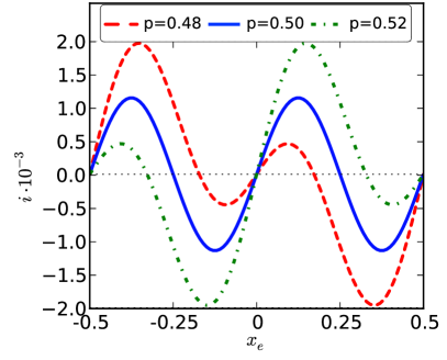
Figure 1: (color online) The dimensionless current $i$ vs the external magnetic flux $x_{e}$ for three values of the probability $p$ of an even number of coherent electrons in the ring. Please note that one can obtain the persistent current for slightly asymmetric case $p=0.48$ just by shifting the presented characteristic for $p=0.52$ by $x_{e}=0.5$. It is the case of ”classical” thermal fluctuations, i.e. when the quantum correction parameter $\lambda_{0}=0$. Other dimensionless parameters are: $\alpha=0.1$, $T_{0}=0.5$, $k_{0}=0.08$.

6 Current – flux characteristics in stationary states

A persistent current is a periodic function of the magnetic flux with a period given by a single-electron flux unit $\phi_{0}=h/e$. To what extent the current is highly sensitive to a variety of subtle effects such as an electron–electron interaction, defects, disorder, coupling to an environment and other degrees of freedom, it is still a topic of controversy and persistent discussion. Fortunately, novel techniques developed recently such as the microtorsional magnetometer harris and scanning SQUID bluhm allow to measure the persistent current in metal rings over a wide range of magnetic fields, temperatures and ring sizes. Like many mesoscopic effects, the persistent current in real systems depends on the particular realization of disorder and thus varies between nominally identical rings, cf. the term $\cos(nk_{F}l)$ in Eq. (9) which in practice is random. In Fig. 1 we depict the well-known dependence of current upon the external magnetic flux $x_{e}$ for three selected values of the probability $p$ of an even number of coherent electrons in the ring. The choice of values of $p$ is arbitrary but shapes of the current are similar to those observed in experiments.

We now focus on the influence of quantum thermal fluctuations on persistent currents. The deviation from the ”classicality” is measured by the dimensionless parameter $\lambda$ which depends on $\lambda_{0}$ (the material constant) and temperature, see Eq. (33). It is instructive to compare basic quantities characterizing the system. In Fig. 2 we show the generalized thermodynamic potential $\Psi_{\lambda}(x)$, the modified diffusion function $D_{\lambda}(x)$ and the stationary probability density $p(x)$ for two values of the quantum correction strength $\lambda_{0}$. Three panels (a), (b) and (c) are presented for the case $x_{e}=0$ (the vanishing external flux). The case $\lambda_{0}=0$ corresponds to classical thermal fluctuations and $\Psi_{0}(x)$ is a bare potential $V(x)/k_{0}T_{0}$. We note that the generalized thermodynamic potential $\Psi_{\lambda}(x)$ for various $\lambda$ changes only slightly. On the contrary, the state-dependent diffusion function is a periodic function of the magnetic flux and possess maxima and minima. It is a radical difference to the classical case $\lambda=0$ for which $D_{0}(x)=D_{0}=k_{0}T_{0}$ is a constant function (thin solid blue line and thin dashed red line in panel (c)). The maxima of $D_{\lambda}(x)$ can be interpreted as a higher effective local temperature. They are located at $x_{e}=1/4\;\mbox{mod}(1/2)$. The impact of quantum corrections on the stationary probability density $p(x)$ seems to be rather insignificant. One can observe a small deformation around the peak of the density: for lower temperature and non-zero $\lambda_{0}$ the peak becomes slightly higher and narrower and the tails do not diverge in the quantum case as fast as in the classical one.

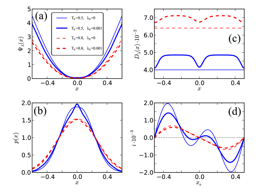
Figure 2: (color online) Four characteristics of the normal metallic ring in the absence (panels a – c) and presence (panel d) of the external flux are demonstrated for two values of the dimensionless temperature: $T_{0}=0.5,0.8$ and for two different values of the quantum fluctuations strength: $\lambda_{0}=0,0.001$. The key for reading this plot is as the following: blue (solid) lines denote curves corresponding to the lower temperature $T_{0}=0.5$ and the red (dashed) lines correspond to the higher temperature $T_{0}=0.8$; the thin lines correspond to $\lambda_{0}=0$ (classical thermal fluctuations) and the thick lines correspond to $\lambda_{0}=0.001$ (quantum thermal fluctuations). In panel (a) we present the thermodynamic potential defined in (29). In the classical case ($\lambda_{0}=0$) it reduces to $V(x)/k_{0}T_{0}$. One can notice only small deviations from the classical case when the rescaled parameter $\lambda_{0}$ is increased to $0.001$. On the panel (b) we illustrate the corresponding stationary probability density function $p(x)$. The bell – shaped curve in the classical limit is slightly deformed for non-zero $\lambda_{0}$. The peak tends to be narrower and reach higher values and the tails decay slower as we increase $\lambda_{0}$. This effect is stimulated collectively by the thermodynamic potential and the effective diffusion presented on panels (a) and (c), respectively. Please note that for the classical case, the flux dependence of $D_{\lambda}(x)$ disappears and constantly equals $k_{0}T_{0}=0.04$ for $T_{0}=0.5$ and $0.064$ for $0.8$. The most significant influence of the temperature is found in panel (d), where the current–flux characteristics are displayed. For small external load, around flux $x_{e}=0$, the system responses in a completely different way for two selected temperatures. For $T_{0}=0.5$ in both classical and quantum cases the persistent current is paramagnetic. If we, however, increase the temperature to $T_{0}=0.8$, the situation changes drastically and the susceptibility for this higher temperature becomes diamagnetic. Other rescaled parameters are set as the following $\alpha=0.1$, $k_{0}=0.08$, $p=0.48$, $\epsilon=100$.

Finally, we analyze the influence of quantum thermal fluctuations on the current-flux characteristics $i=i(x_{e})$. It is illustrated in panel (d) of Fig. 2 and in Fig. 3. Two solid blue lines in panel (d) of Fig. 2 are qualitatively similar to the experimental curve shown in figure S6(A) in the Supporting Online Material supp of the paper harris . We observe that in all cases of quantum thermal fluctuations the amplitude of persistent currents is reduced in comparison to classical thermal fluctuations case ($\lambda_{0}=0$) both in the paramagnetic regime ($T_{0}=0.5$) and diamagnetic regime ($T_{0}=0.8$). The parameter regime depicted in Fig. 3 is much more interesting. For $T_{0}=0.6$, in the ”classical” case, the persistent current is paramagnetic, i.e. $i=\eta x_{e}$ with the positive slope $\eta>0$ in the vicinity of $x_{e}=0$. It is a linear response regime where the transport coefficient (susceptibility) $\eta=\lim_{x_{e}\to 0}[i(x_{e})/x_{e}]$.

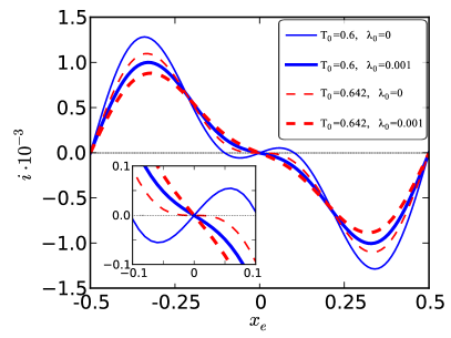
Figure 3: (color online) The dimensionless current $i$ vs the external magnetic flux $x_{e}$ for two values of the dimensionless temperature $T_{0}=0.6,0.642$ and two values of the parameter $\lambda_{0}=0$ (classical thermal fluctuations) and $0.001$ (quantum thermal fluctuations). Again, the key for reading this plot is as for the previous figure: blue (solid) lines denote curves corresponding to the lower temperature $T_{0}=0.6$ and the red (dashed) lines correspond to the higher temperature $T_{0}=0.642$; the thin lines correspond to $\lambda_{0}=0$ and thick lines corresponds to $\lambda_{0}=0.001$. The most significant influence of the ’quantum parameter’ $\lambda_{0}$ is found for the rescaled temperature $T_{0}=0.6$, where the current $i$ changes its behavior from paramagnetic to diamagnetic one just by adjusting $\lambda_{0}$ from $0$ to $0.001$. Moreover, for the presented set of the system parameters we can find characteristic cross-temperature at $T_{0}=0.642$ where the magnetic susceptibility is zero in the classical case and diamagnetic in quantum, see red (dashed) line for details. Rescaled parameters are set as the following $\alpha=0.1$, $k_{0}=0.08$, $p=0.48$, $\epsilon=100$.

If temperature is a litlle bit higher ($T_{0}=0.642$), the susceptibility $\eta=0$ zero in the classical case. If quantum corrections are taken into account, the susceptibility $\eta<0$ , the slope of the $i-x_{e}$ curve in negative and the current becomes diamagnetic. The most interesting observation is that the persistent current can change its character from the paramagnetic to diamagnetic phase and the sign of the low-field magnetic response depends on the level of the quantum corrections. Our detailed numerical analysis shows that the sign of magnetic susceptibility can easily be affected by system parameters and therefore is not robust against small perturbations. This is what has been observed in many experiments regarding the paramagnetic or/and diamagnetic persistent currents. The best illustration of what we state here is the response of 15 nominally identical ring presented in Fig. 2 in Ref. bluhm : e.g. for the ring 1 the current is paramagnetic while for the ring 2 it is diamagnetic.

7 Conclusions

In many cases and for various systems at the ”intermediate” temperatures, the semi-classical theory is insufficient and the quantum corrections should be involved. It has been shown in the literature that in the strong friction limit, the quantum effects are restricted not only to low temperatures and therefore they should be incorporated for the higher temperatures as well. This is so because the quantum fluctuations, even if reduced for one variable, are enlarged for the conjugate variable. The dynamics as well as the stationary states in this regime can be modeled by the quantum Smoluchowski equation. In other words, the quantum non-Markovian stochastic process is approximated by the classical Markovian process with the modified, state-dependent diffusion function.

The role of the quantum corrections on the current-flux characteristics is addressed in this work. A general conclusion is that the quantum thermal fluctuations reduce the amplitude of the persistent currents: the current amplitude is always smaller than the corresponding ”classical” one. In the quantum case, the diffusion constant becomes a periodic function of the magnetic flux. Maxima and minima of the diffusion function can be interpreted in terms of the higher and lower local temperature. There are parameters regimes where the system response changes the character from the paramagnetic to diamagnetic, when the quantum effects of thermal fluctuations increases. It would be interesting to extend the current study by including the time-dependent drivings modeled by the time-periodic magnetic fields. One could expect novel transport phenomena like a negative susceptibility which for Brownian particles corresponds to negative mobility mach or negative conductances kos .

References

- (1) F. Hund, Ann. Phys. (Leipzig) 32, 102 (1938).
- (2) I. O. Kulik, JETP Lett. 11, 275 (1970); M. Büttiker, Y. Imry, R. Landauer, Phys. Lett. A 96, 365 (1993).
- (3) L. P. Lévy, G. Dolan, J. Dunsmuir, and H. Bouchiat, Phys. Rev. Lett. 64, 2074 (1990).
- (4) V. Chandrasekhar, R. A. Webb, M. J. Brandy, M. B. Ketchen, W. J. Gallagher, and A. Kleinsasser, Phys. Rev. Lett. 67, 3578 (1991); D. Mailly, C. Chapelier and A. Benoit, Phys. Rev. Lett. 70, 2020 (1993); B. Reulet, M. Ramin, H. Bouchiat, and D. Mailly, Phys. Rev. Lett. 75, 124 (1995); E. M. Q. Jariwala, P. Mohanty, M. B. Ketchen, R. A. Webb, Phys. Rev. Lett. 86, 1594 (2001); W. Rabaut, L. Saminadayar, D. Mailly, K. Hasselbach, A. Benoît, B. Etienne, Phys. Rev. Lett. 86, 3124 (2001); R. Deblock, R. Bel, B. Reulet, H. Bouchiat, D. Mailly, Phys. Rev. Lett. 89, 206803 (2002).
- (5) A. C. Bleszynski-Jayich, W. E. Shanks, B. Peaudecerf, E. Ginossar, F. von Oppen, L. Glazman, and J. G. E. Harris, Science 326, 272 (2009).
- (6) H. Bluhm, N. C. Koshnick, J. A. Bert, M. E. Huber, and K. A. Moler, Phys. Rev. Lett. 102, 136802 (2009).
- (7) J. Dajka, L. Machura, S, Rogoziński, and J. Łuczka, Phys. Rev. B 76, 045337 (2007); J. Dajka, S. Rogoziński, Ł. Machura, J. Łuczka, Acta Physica Polonica B 38, 1737 (2007); L. Machura, J. Dajka, and J. Łuczka, J. Stat. Mech. P01030 (2009).
- (8) A. Barone, G. Paterno, Physics and applications of the Josephson effect, Wiley, New York (1982)
- (9) A. Neiman, L. Schimansky-Geier, T. Vadivasova, V. S. Anishchenko, V. Astakhov, Nonlinear Dynamics of Chaotic and Stochastic Systems, Springer, Berlin (2007); J. Łuczka, M. Niemiec and E. Piotrowski, Phys. Lett. A 167, 475 (1992).
- (10) J. Ankerhold, P. Pechukas, H. Grabert, Phys. Rev. Lett. 87, 086801 (2001).
- (11) Ł. Machura, M. Kostur, P. Hänggi, P. Talkner, J. Łuczka Phys. Rev. E 70, 031107 (2004); J. Łuczka, R. Rudnicki, P. Hänggi, Physica A 351, 60 (2005).
- (12) J. Ankerhold, Europhys. Lett. 67, 280 (2004); J. Ankerhold, P. Pechukas, H. Grabert, Chaos 15, 026106 (2005); S. A. Maier and J. Ankerhold, Phys. Rev. E 81, 021107 (2010) .
- (13) W. T. Coffey, Y. P. Kalmykov, S. V. Titov, and L. Cleary, Phys. Rev. E 78, 031114 (2008); Phys. Rev. B 79, 054507 (2009); L. Cleary, W. T. Coffey, Y. P. Kalmykov, and S. V. Titov, Phys. Rev. E 80, 051106 (2009).
- (14) M. Kostur, L. Machura, P. Talkner, P. Hänggi, J. Łuczka, Phys. Rev. B 77, 104509 (2008).
- (15) H.F. Cheung, Y. Gefen, E.K. Riedel and W.H. Shih Phys. Rev. B 37 ,6050 (1989).
- (16) P. Kopietz, Phys. Rev. Lett. 70, 3123 (1993).
- (17) Y. Imry, B.L. Altshuhler, in Nanostructures and Mesoscopic Phenomena, eds. W.P. Kirk and M.A. Reed, Academic San Diego (1992).
- (18) A. A. Aligia, Phys. Rev. B 66, 165303 (2002); Guo–Hui Ding and Bing Dong, Phys. Rev. B 67, 195327 (2003).
- (19) M. Büttiker, Physica Scripta T54, 104 (1994).
- (20) C.W. Gardiner, Handbook of stochastic methods, Springer, Berlin (1983).
- (21) Supporting Online Material for Ref. harris : www.sciencemag.org/cgi/content/full/326/5950/272/DC1.
- (22) M. Kostur, L. Machura, P. Hänggi, J. Łuczka and P. Talkner, Physica A 371, 20 (2006).