The Temperature Dependence of Solar Active Region Outflows

Abstract

Spectroscopic observations with the EUV Imaging Spectrometer (EIS) on Hinode have revealed large areas of high speed outflows at the periphery of many solar active regions. These outflows are of interest because they may connect to the heliosphere and contribute to the solar wind. In this Letter we use slit rasters from EIS in combination with narrow band slot imaging to study the temperature dependence of an active region outflow and show that it is more complicated than previously thought. Outflows are observed primarily in emission lines from Fe XI–Fe XV. Observations at lower temperatures (Si VII), in contrast, show bright fan-like structures that are dominated by downflows. The morphology of the outflows is also different than that of the fans. This suggests that the fan loops, which often show apparent outflows in imaging data, are contained on closed field lines and are not directly related to the active region outflows.

1. Introduction

The detection of large areas of high speed outflows at the periphery of many solar active regions is one of the more intriguing discoveries of the EUV Imaging Spectrometer (EIS) on Hinode (e.g., Doschek et al., 2007, 2008; Harra et al., 2008; Del Zanna, 2008). These outflows are characterized by bulk shifts in the line profile of up to 50 km s^-1 and enhancements in the blue wing of up to 200 km s^-1 (Bryans et al., 2010; McIntosh & De Pontieu, 2009). These outflow regions are of interest because they may lie on open field lines that connect to the heliosphere and contribute to the solar wind (e.g., Schrijver & De Rosa, 2003).

One aspect of the active region outflows that has not been investigated in sufficient detail is their temperature dependence. Spectroscopic observations have generally identified outflows in relatively hot coronal lines (Fe XII–Fe XV). Several studies, however, have associated active region outflows with the apparent motions observed along cooler, fan-like structures using imaging instruments (e.g., Sakao et al., 2007; Hara et al., 2008; McIntosh & De Pontieu, 2009; He et al., 2010).

In this Letter we use a combination of slit rasters and narrow band slot images to study the temperature dependence of outflows in an active region. Using EIS slit rasters we find that at lower temperatures (Si VII) the emission from the fans is strongly red-shifted, suggesting that this downflowing material lies on closed field lines. This interpretation is consistent with larger field of view images which suggest that the fan loops connect to the quiet Sun or to other active regions. At intermediate temperatures (Fe X) we see a mixture of outflows and downflows. Outflows are observed from Fe XI–Fe XV. The velocities presented here are based on new relative rest wavelengths derived from EIS observations from the quiet corona above the limb. EIS slot imaging, which provides observations of 1 Å spectral bands over a wider field of view, is consistent with these findings. EIS slot movies of this region in Fe XII show apparent outflows while slot movies in Si VII show apparent downflows.

2. Observations

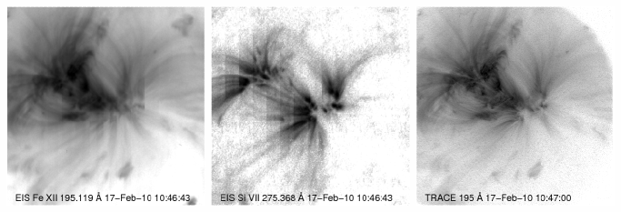
Figure 1.— (left panels) EIS slot rasters in Fe XII 195.119 Å and Si VII 275.368 Å. The slot rasters are constructed by stepping the 40″ slot across the active region. (right panel) An approximately co-temporal TRACE 195 Å image. The electronic version of the manuscript contains EIS and TRACE movies. The EIS slot movies show apparent outflows in Fe XII and apparent downflows in Si VII. The intensities are shown with a reversed color table where bright features are black.

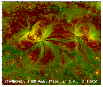
Figure 2.— A two-color, wavelet enhanced EUVI image of active region 11048. The 195 Å is red and the 171 Å image is green. This image illustrates the various types of connections for the fan loops. Some fan loops connect to another active region, some loops connect to the quiet Sun, while others connect to the opposite polarity flux within the active region itself. The electronic version of the manuscript contains an animation of these data from 7–21 February 2010.

The EIS instrument on Hinode is a high spatial and spectral resolution imaging spectrograph. EIS observes two wavelength ranges, 171–212 Å and 245–291 Å, with a spectral resolution of about 22 mÅ and a spatial resolution of about 1″ per pixel. There are 1″ and 2″ slits as well as 40″ and 266″ slots available. Solar images can be made using one of the slots or by stepping one of the slits over a region of the Sun. Telemetry constraints generally limit the spatial and spectral coverage of an observation. See Culhane et al. (2007) and Korendyke et al. (2006) for more details on the EIS instrument.

For this analysis we consider two different EIS observing sequences that were run on NOAA active region 11048. One sequence involves constructing a raster by stepping the 1″ slit across a small region of the Sun ($180\arcsec\times 512\arcsec$) taking a 50 s exposure at each position. To accelerate the observing a 3″ step was taken between exposures. Emission lines of interest were selected and fit with a single Gaussian. Measuring absolute velocities with EIS is difficult and we will discuss this in detail in the next section. This observing sequence was run 6 times during a two day period. Here we present results from the run that began at 04:25 UT and ended at 05:17 UT on 17 February 2010.

The second observing sequence involves constructing a series of relatively high cadence rasters using the 40″ slot. The 40″ slot provides a dispersed image similar to those taken with the SO82-A instrument on Skylab (Tousey et al., 1977). The relatively narrow 40″ width of the EIS slot, however, yields images which integrate over only 1 Å of the solar spectrum. This limits the amount of overlap between images. To build up a larger field of view the slot is stepped across the Sun and, for this observing program, a 10 s exposure is taken at each position. The observing program of interest here took a series of 14 exposures for each raster. The final field of view is about $448\arcsec\times 480\arcsec$. The time between successive slot rasters is about 180 s. In this paper we present results from a run that began at 10:45 UT and ended at 15:30 UT on 17 February 2010.

We also consider context observations from the Transition Region and Coronal Explorer (TRACE, see Handy et al. 1999) and the EUV Imager (EUVI) on the Solar Terrestrial Relations Observatory (STEREO, see Howard et al. 2008). Both TRACE and EUVI are high resolution EUV multi-layer telescopes with four different channels. For both instruments there are three channels for imaging the corona: Fe IX/Fe X 171 Å, Fe XII 195 Å, and Fe XV 284 Å. The TRACE observations of interest here consisted primarily of full resolution 195 Å images. The median cadence was 47 s, but there were several extended data gaps. These observations were taken from 10:00 UT to 16:00 UT on 17 February 2010. The EUVI images we have studied are from the behind spacecraft and show the evolution of the active region of interest from 7–21 February 2010. The separation angle between Earth and STEREO B was about 71^∘ on 17 February 2010.

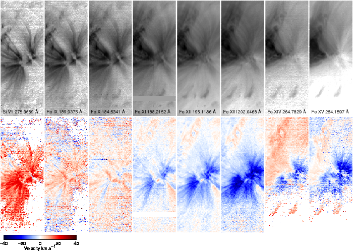
Figure 3.— EIS observations of active region outflows on 2010 February 17. The top panels show the intensities derived from Gaussian fits to the line profiles. The intensities are shown with a reversed color table. The bottom panels show the Doppler shifts relative to the quiet Sun in each line. Velocities for very weak line profiles have been “grayed out”. The relative wavelengths are from the measurements presented in Table 1. The velocities show a progression from downflows at low temperatures to strong outflows at higher temperatures with a transition region around Fe X.

3. Results

EIS slot rasters from the Fe XII 195.119 Å and Si VII 275.368 Å emission lines are shown in Figure 1. Movies of these EIS data are available in the electronic version of the manuscript. The movies show clear evidence for dynamical behavior in both the cool fan loops that are bright in Si VII and in the faint regions seen in Fe XII. The apparent motions seen in Si VII are suggestive of downflows. The apparent motions in Fe XII, in contrast, suggest highly episodic outflows.

Also shown in Figure 1 is a nearly simultaneous TRACE 195 Å image from this region. The TRACE movie of these data, which is included in the electron version of the manuscript, is generally consistent with the EIS slot data and shows apparent outflows. We note that the while the fans are generally observed at lower temperatures, they can also appear in 195 Å images. The 195 Å bandpass includes some cooler emission lines, such as Fe VIII 194.663 Å, which can be comparable in intensity to the Fe XII 195.119 Å line in the fan loops (e.g., Landi & Young, 2009; Del Zanna & Mason, 2003). Thus the temperature of the emission imaged in the 195 Å channel is ambiguous.

The connectivity of the fan loops is unclear in the small field of view EIS and TRACE images. In Figure 2 we show a larger field of view of this active region extracted from a full Sun EUVI image. This image is a combination of wavelet enhanced 195 Å and 171 Å images. The multi-scale wavelet processing enhances the loops by removing the diffuse background and sharpening the remaining signal (Stenborg et al., 2008). These images suggest that the fan loops lie on closed field lines and illustrate the various types of connections that these loops can have. The fan loops appear to connect to flux within the active region, other active regions, and the quiet Sun. A movie of these data are available in the electronic version of the manuscript.

EIS intensity maps derived from the slit observations are shown in Figure 3. As expected from the narrow bandpasses of the EIS slot images, the intensity maps show essentially the same morphology as the corresponding slot images. The additional lines available with the slit allow us to study the morphology of the flows as a function of temperature. The fan loops are dominated by cool emission and are bright in Si VII, Fe IX, and Fe X. The morphology of the outflow region seen in the Fe XII 195.119 Å slot movies is echoed in all of the emission at intermediate temperatures (Fe XI–Fe XIII). At the highest temperatures considered here (Fe XIV and Fe XV) the emission is relatively weak in the outflow region, although generally above the level of the quiet Sun.

Also shown in Figure 3 are the Doppler velocity maps derived from the slit data. The Doppler velocity maps in Si VII and Fe XII are consistent with the apparent motions seen in the movies, with strong downflows in Si VII and strong outflows in Fe XII. The Doppler maps also suggest that there is a transition from downflows to outflows around Fe X. Our observations of strong downflows at low temperatures in the fans are consistent with previous measurements of downflows in active region fan loops in Ne VIII by Winebarger et al. (2002).

Table 1Relative Wavelengths Observed With EIS

Line	$\lambda$	$\sigma_{\lambda}$	$\sigma_{v}$	$\delta_{\lambda}$	$\delta_{v}$
Fe VIII 185.213	185.2107	0.5	0.9	2.3	3.7
Fe VIII 186.601	186.6060	0.7	1.1	-5.0	-8.0
Fe VIII 194.663	194.6523	0.7	1.1	10.7	16.5
Fe IX 189.941	189.9375	0.4	0.7	3.5	5.5
Fe IX 197.862	197.8570	0.3	0.5	5.0	7.5
Fe X 184.536	184.5341	0.4	0.6	1.9	3.0
Fe XI 180.401	180.3990	0.3	0.5	2.0	3.4
Fe XI 188.216	188.2152	0.2	0.2	0.8	1.3
Fe XI 188.299	188.3004	0.2	0.2	-1.4	-2.2
Fe XII 192.394	192.3940	0.0	0.0	0.0	0.0
Fe XII 193.509	193.5090	0.1	0.2	0.0	0.1
Fe XII 195.119	195.1186	0.1	0.2	0.4	0.7
Fe XIII 202.044	202.0468	0.2	0.2	-2.8	-4.1
Fe XIII 203.826	203.8243	0.6	0.9	1.7	2.5
Si VII 275.368	275.3669	0.7	0.7	1.1	1.2
Si X 253.791	253.7874	1.1	1.3	3.6	4.2
Si X 258.375	258.3750	0.0	0.0	0.0	0.0
Si X 261.058	261.0573	0.6	0.6	0.7	0.8
Si X 271.990	271.9902	0.4	0.4	-0.2	-0.3
Si X 277.265	277.2611	0.6	0.6	3.9	4.2
Fe XIV 211.316	211.3192	0.6	0.9	-3.2	-4.6
Fe XIV 264.787	264.7829	0.6	0.7	4.1	4.7
Fe XIV 270.519	270.5223	0.4	0.5	-3.3	-3.7
Fe XIV 274.203	274.2021	0.7	0.7	0.9	0.9
Fe XV 284.160	284.1597	1.0	1.0	0.3	0.3

There are several difficulties with measuring Doppler velocities with EIS and it is important to outline the steps involved in computing them. One difficulty is the lack of absolutely calibrated rest wavelengths for the emission lines observed at these wavelengths. Tabulations of line identifications in the EIS wavelength ranges, (e.g., Brown et al., 2008), use wavelengths from previous solar observations, such as the Behring et al. (1976) rocket flight, and already include any systematic Doppler shifts. Thus even if the EIS wavelength calibration was known very precisely, velocity measurements relative to an absolute standard would still be impossible. The best we can do is to consider relative velocity measurements.

There has been some work on the relative wavelengths of the emission lines measured with EIS (e.g., Brown et al., 2008), but none that includes observations of the quiet corona above the limb, where we expect the line of sight velocities to be small for all lines. To investigate the relative wavelengths systematically we have analyzed data from another observing sequence that was run on the 18 May 2010 beginning at 11:14 UT. In this sequence a series of 120 s exposures are taken with the 1″ slit and the full CCD is telemetered to the ground. This series of deep exposures provide good statistics for all of the lines of interest. This means that the measured relative wavelengths are largely independent of the slit tilt and the orbital variation. For each line of interest we have performed the same Gaussian fitting that was used for the slit raster data. For completeness we also consider several additional lines that were not included in the raster data. From these fits we calculate the median and the 1-$\sigma$ variance in the measured centroid for each line. For each exposure the wavelengths are measured relative to the Fe XII 192.394 Å and Si X 258.375 Å lines.

These new relative wavelengths are given in Table 1 and show that the centroids measured in the quiet corona above the limb are generally consistent with the values in the literature (Brown et al., 2008) to 4 mÅ or better. There are, however, several important lines for which there are discrepancies. For example, the wavelength for the Fe XIII 202.044 Å line needs to be adjusted to 202.0468 Å (a difference of 4.1 km s^-1) to provide velocities that are consistent with the Fe XII 192, 193, and 195 Å lines. We also note that there is a typographical error in Brown et al. (2008), who give the wavelength for Si VII as 275.352 Å. Behring et al. (1976) give the wavelength of this line as 275.368 Å, consistent with our result of 275.3669 Å.

Another correction that needs to be made accounts for the fact that the EIS slit is slightly tilted relative to the columns of the CCD. The magnitude of the slit tilt has been calculated for each pixel along the slit using extensive observations of emission lines above the limb in the quiet corona, where we expect the velocities to be uniform (Kamio et al., 2010).

Perhaps the most significant difficulty with EIS velocity measurements is that the spectra drift back and forth across the detector during the satellite orbit of 98 minutes with an amplitude of around 2 wavelength pixels (e.g., Brown et al., 2007). This behavior is thought to be due to the changing thermal environment of the satellite during an orbit.

To make an initial correction to the wavelength scale we use the spectral drift-spacecraft temperature model derived by Kamio et al. (2010). This model is based on the results from an artificial neural network that was trained on measurements of the Fe XII 195.119 Å centroid and temperature measurements taken within the instrument. This procedure corrects the wavelength scale based on the assumption that there are no net velocities in this line in the quiet corona. Peter & Judge (1999), however, find that coronal lines are weakly blueshifted in the quiet Sun by around 2–5 km s^-1. These values are much smaller than the high velocity upflows and downflows that we are concerned with in this paper.

To further refine the wavelength scale we chose an emission line from each wavelength band and compute a spatially averaged line profile in a quiet region from each exposure. The wavelength scale is adjusted so there are no net velocities across the raster in these lines. For this procedure we use the Si VII 275.368 Å and Fe XII 195.119 Å lines. This procedure also verifies that the initial velocity correction has largely removed the temporal variability in the centroid. The differences between the centroid of the average profiles and the wavelength given in Table 1 are essentially constant with time. The systematic application of these new relative wavelengths and correction techniques to other EIS observations will be presented in a future paper.

Given the extensive processing of the data needed to compute the line centroids, the absolute velocities should be considered with caution. The large downflows observed in Si VII and the large upflows observed Fe XI–Fe XIII are very robust results. Some of the details are far less certain. The weak redshifts seen in Fe X, for example, could easily be weak blueshifts. The conservative interpretation is that there is a transition between upflows and downflows in the temperature range where Fe IX and Fe X are formed. The extension of the outflows to Fe XV should also be regarded with caution.

Figure 4.— EIS observations of active region outflows on 2007 February 20. This region has been considered by Sakao et al. (2007), Hara et al. (2008), McIntosh & De Pontieu (2009), and He et al. (2010). The bright fan loops that are bright in Fe VIII and Si VII are dominated by downflows while outflows are observed at higher temperatures. Note that Fe VIII 185.213 Å is blended with a weak Ni XVI line, which influences the fits in the high temperature core of the active region.

4. Summary and Discussion

We have presented systematic observations of an active region outflow observed with EIS using both narrow band slot imaging and slit rasters. These observations show that the outflow region has a complex velocity structure with strong downflows being observed at relatively cool temperatures and outflows being observed at higher temperatures. The presence of downflows on the fan loops suggests cooling plasma trapped on closed field lines. This interpretation is consistent with the larger field of view STEREO EUVI images of this region.

Earlier studies comparing outflows observed with EIS and simultaneous imaging data, (e.g., Sakao et al., 2007; Hara et al., 2008; McIntosh & De Pontieu, 2009; He et al., 2010), have associated active region outflows with the apparent motions observed along the fan loops using broad-band imaging instruments, such as TRACE 171 Å and 195 Å. Interestingly, these previous studies have all considered the same region but have not presented a full set of Doppler maps from EIS. In light of this we have analyzed data from this region using the methods outlined in the previous section. The intensity and Doppler maps, which are shown in Figure 4, are consistent with our results. The bright cool loops are dominated by inflows and the outflows occur at higher temperatures.

So how do we form a coherent picture from these results? We conjecture that the fan loops and the outflows form two largely independent populations. In this view the fan loops imaged in Si VII are closed structures and some of the dynamics observed at higher temperatures are related to the heating and cooling of the plasma along these field lines (see Ugarte-Urra et al. 2009). Furthermore, we speculate that most of the outflows lie on open field lines that connect to the heliosphere. The fact that the fan loops and the outflows tend to occur in the same general area of an active region could be related to the changes in magnetic topology that occur there (Baker et al., 2009; Schrijver et al., 2010).

References

- (1)
- 08 (1) 08. 1
- Baker et al. (2009) Baker, D., van Driel-Gesztelyi, L., Mandrini, C. H., Démoulin, P., & Murray, M. J. 2009, ApJ, 705, 926
- Behring et al. (1976) Behring, W. E., Cohen, L., Doschek, G. A., & Feldman, U. 1976, ApJ, 203, 521
- Brown et al. (2008) Brown, C. M., Feldman, U., Seely, J. F., Korendyke, C. M., & Hara, H. 2008, ApJS, 176, 511
- Brown et al. (2007) Brown, C. M., et al. 2007, PASJ, 59, 865
- Bryans et al. (2010) Bryans, P., Young, P. R., & Doschek, G. A. 2010, ApJ, 715, 1012
- Culhane et al. (2007) Culhane, J. L., et al. 2007, Sol. Phys., 243, 19
- Del Zanna (2008) Del Zanna, G. 2008, A&A, 481, L49
- Del Zanna & Mason (2003) Del Zanna, G., & Mason, H. E. 2003, A&A, 406, 1089
- Doschek et al. (2007) Doschek, G. A., et al. 2007, ApJ, 667, L109
- Doschek et al. (2008) Doschek, G. A., Warren, H. P., Mariska, J. T., Muglach, K., Culhane, J. L., Hara, H., & Watanabe, T. 2008, ApJ, 686, 1362
- Handy et al. (1999) Handy, B. N., et al. 1999, Sol. Phys., 187, 229
- Hara et al. (2008) Hara, H., Watanabe, T., Harra, L. K., Culhane, J. L., Young, P. R., Mariska, J. T., & Doschek, G. A. 2008, ApJ, 678, L67
- Harra et al. (2008) Harra, L. K., Sakao, T., Mandrini, C. H., Hara, H., Imada, S., Young, P. R., van Driel-Gesztelyi, L., & Baker, D. 2008, ApJ, 676, L147
- He et al. (2010) He, J., Marsch, E., Tu, C., Guo, L., & Tian, H. 2010, A&A, 516, A14
- Howard et al. (2008) Howard, R. A., et al. 2008, Space Science Reviews, 136, 67
- Kamio et al. (2010) Kamio, S., Hara, H., Watanabe, T., Fredvik, T., & Hansteen, V. H. 2010, ArXiv e-prints
- Korendyke et al. (2006) Korendyke, C. M., et al. 2006, Appl. Opt., 45, 8674
- Landi & Young (2009) Landi, E., & Young, P. R. 2009, ApJ, 706, 1
- McIntosh & De Pontieu (2009) McIntosh, S. W., & De Pontieu, B. 2009, ApJ, 706, L80
- Peter & Judge (1999) Peter, H., & Judge, P. G. 1999, ApJ, 522, 1148
- Sakao et al. (2007) Sakao, T., et al. 2007, Science, 318, 1585
- Schrijver & De Rosa (2003) Schrijver, C. J., & De Rosa, M. L. 2003, Sol. Phys., 212, 165
- Schrijver et al. (2010) Schrijver, C. J., DeRosa, M. L., & Title, A. M. 2010, ApJ, submitted
- Stenborg et al. (2008) Stenborg, G., Vourlidas, A., & Howard, R. A. 2008, ApJ, 674, 1201
- Tousey et al. (1977) Tousey, R., Bartoe, J., Brueckner, G. E., & Purcell, J. D. 1977, Appl. Opt., 16, 870
- Ugarte-Urra et al. (2009) Ugarte-Urra, I., Warren, H. P., & Brooks, D. H. 2009, ApJ, 695, 642
- Winebarger et al. (2002) Winebarger, A. R., Warren, H., van Ballegooijen, A., DeLuca, E. E., & Golub, L. 2002, ApJ, 567, L89