Orbital structure of quarks inside the nucleon in the light-cone diquark model

Abstract

We study the orbital angular momentum structure of the quarks inside the proton. By employing the light-cone diquark model and the overlap representation formalism, we calculate the chiral-even generalized parton distribution functions (GPDs) $H_{q}(x,\xi,\Delta^{2})$, $\widetilde{H}_{q}(x,\xi,\Delta^{2})$ and $E_{q}(x,\xi,\Delta^{2})$ at zero skewedness for $q=u$ and $d$ quarks. In our model $E_{u}$ and $E_{d}$ have opposite sign with similar size. Those GPDs are applied to calculate the orbital angular momentum (OAM) distributions, showing that $L_{u}(x)$ is positive, while $L_{d}(x)$ is consistent with zero compared with $L_{u}(x)$. We introduce the impact parameter dependence of the quark OAM distribution. It describes the position space distribution of the quark orbital angular momentum at given $x$. We found that the impact parameter dependence of the quark OAM distribution is axially symmetric in the light-cone diquark model.

I introduction

understanding the spin structure of the nucleon is one of the most important challenges in hadron physics. The naive picture that the nucleon spin is provided totally by the spin of its three valence quark was proved to be wrong by the experimental measurements. The EMC result emc indicates that a large fraction of the nucleon spin is carried by other sources of angular momentum. There have been many attempts to explain the EMC result from the fundamental theory. Besides the angular momentum of the gluon, the quark orbital angular momentum (OAM) Sehgal:1974rz is believed to provide a substantial part of the nucleon spin. In the last two decades the theoretical description of the quark OAM distribution has been established orbital ; ji97 ; hagler98 ; kundu99 ; Ma:1998ar . It has been shown by Ji that the quark angular momentum can be separated into ji97 the usual quark helicity and a gauge-invariant orbital contributions $L_{q}$. One of the advantage of this decomposition is that $L_{q}$ is related to generalized parton distributions (GPDs) Mueller:1998fv ; Ji:1996nm ; Radyushkin:1997ki ; diehl03 ; Belitsky:2005qn ; Boffi:2007yc , the experimental observables that enter the descriptions of hard exclusive processes, such as deeply virtual Compton processes Radyushkin:1996nd ; Ji:1996nm and meson exclusive production Polyakov:1998ze ; Collins:1996fb .

Moreover, recently it has been found that the quark OAM plays an essential role through spin-orbit correlations in some novel phenomena that appear in the physics of single spin asymmetries, among which a particular transverse momentum distribution (TMD) Mulders:1995dh ; Boer:1997nt —- Sivers function Sivers:1989cc ; Sivers:1990fh —-has attracted a lot of interest, since it is an essential piece in our understanding of the single spin asymmetries (SSA) observed in semi-inclusive deeply inelastic scattering (SIDIS). These SSAs have been measured recently by both the HERMES Airapetian:2004tw ; hermes05 and COMPASS compass ; compass06 Collaborations. An interesting observation is that there is a quantitative relation amm ; Burkardt:2005km ; ls07 between the Sivers function $f_{1T}^{\bot q}$ and the GPD $E^{q}$, although it is obtained in a model dependent way, suggesting that similar underlying physics plays a role for nonzero $f_{1T}^{\bot q}$ and $E^{q}$. Similar relations have been obtained between Boer-Muldes functions and chiral-odd quark GPDs Diehl:2005jf ; Gockeler:2006zu . A complete study on the relations between the GPDs and TMDs has been presented in gpdtmd , which becomes more transparent through the conception of general parton correlation functions Meissner:2008ay ; Meissner:2009ww . The relations between GPDs and TMDs are more intuitive Burkardt:2002ks ; Burkardt:2003uw if we interpret GPDs in the transverse position (impact parameter) space Burkardt:2000za ; Burkardt:2002hr ; Diehl:2002he ; Burkardt:2003je . Of particular interest is the case of zero skewedness ($\xi=0$), where a density interpretation of GPDs in impact parameter space may be obtained Burkardt:2000za . In particular this interpretation allows one to study a three-dimensional picture of the nucleon.

In this paper, we study the orbital angular momentum structure of the quarks inside the proton in a light-cone diquark model. In this model the light-cone wave function of the proton can be obtained. It is then convenient to express the physical observables in the overlap representation formalism Brodsky:2000xy ; Diehl:2000xz . We calculate the chiral-even generalized parton distribution functions (GPDs) $H_{q}(x,\xi,\Delta^{2})$, $\widetilde{H}_{q}(x,\xi,\Delta^{2})$ and $E_{q}(x,\xi,\Delta^{2})$ at the zero skewedness for $q=u$ and $d$. We found that $E_{u}$ and $E_{d}$ have opposite sign with similar size in this model. The GPDs are applied to calculate the quark OAM distributions, showing that $L_{u}(x)$ is positive, while $L_{d}(x)$ is consistent with zero compared with $L_{u}(x)$, and the net OAM of the $u$ and $d$ quarks is positive. We also introduce the impact parameter dependence of quark OAM distribution. It describes the position space distribution of the quark OAM at given $x$. We found that the impact parameter dependence of quark OAM distribution is axially symmetric in the light-cone diquark model.

The manuscript is organized in the following way. In Section. II we review the GPDs and their connections with quark orbital angular momentum, in Section III, we present the calculation of chiral-even GPDs from the light-cone diquark model, by applying the overlap representation formalism. We also show the calculation of the quark OAM in the same approach. In Section IV we introduce the impact parameter dependence of quark OAM distribution and present results of the position space distribution for orbiting $u$ quark, from the light-cone diquark model. We summarize our paper in Section V.

II systematics of generalized parton distributions and the orbital angular momentum

GPDs are introduced to describe the exclusive process in which the momenta of the incoming and outgoing nucleon in the symmetric frame are given by

$$p=P+\tfrac{1}{2}\Delta\,,\qquad p^{\prime}=P-\tfrac{1}{2}\Delta\,,$$ (1)

and satisfy $p^{2}=p^{\prime 2}=M^{2}$, with $M$ denoting the nucleon mass. The GPDs depend on the following variables

$$x=\frac{k^{+}}{P^{+}}\,,\qquad\xi=-\frac{\Delta^{+}}{2P^{+}}\,,\qquad t=\Delta^{2}\,,$$ (2)

where the light-cone coordinates are defined by

$$a^{\pm}=(a^{0}\pm a^{3})\,,\qquad\vec{a}_{T}=(a^{1},a^{2})$$ (3)

for a generic 4-vector $a$. In a physical process the so-called skewness $\xi$ and the momentum transfer $t$ to the nucleon are fixed by the external kinematics, whereas $x$ is typically an integration variable.

The chiral-even GPDs $H_{q}$, $E_{q}$ and ${\widetilde{H}}_{q}$, ${\widetilde{E}}_{q}$ for quarks are defined through matrix elements of the bilinear vector and axial vector currents on the light-cone:

$$\int\frac{dy^{-}}{8\pi}\;e^{ixP^{+}y^{-}/2}\;\langle p^{\prime}|\bar{\psi}(0)\,\gamma^{+}\,\psi(y)\,|p\rangle\Big{|}_{y^{+}=0,y_{\perp}=0}$$

$$= {1\over 2P^{+}}\ {\bar{U}}(p^{\prime})\left(\,\ {\gamma^{+}}H(x,\xi,t)+\ {i\sigma^{+\mu}\Delta_{\mu}\over 2M}E(x,\xi,t)\,\right)U(p)\ ,$$

$$\int\frac{dy^{-}}{8\pi}\;e^{ixP^{+}y^{-}/2}\;\langle p^{\prime}|\bar{\psi}(0)\,\gamma^{+}\gamma_{5}\,\psi(y)\,|p\rangle\Big{|}_{y^{+}=0,y_{\perp}=0}$$

$$= {1\over 2P^{+}}\ {\bar{U}}(p^{\prime})\left(\,\ {\gamma^{+}\gamma_{5}}{\widetilde{H}}(x,\xi,t)+\ {\Delta^{+}{\gamma_{5}}\over 2M}\,{\widetilde{E}}(x,\xi,t)\,\right)U(p)\ .$$

An important implication of GPDs is that they are related to the OAM (OAM ) of the quark, which is expected to provide essential contribution to the total spin of the nucleon. Here we follow the decomposition of the nucleon spin introduced by Ji ji97 :

$$J^{z}=J_{q}^{z}+J_{g}^{z}=\frac{1}{2}\sum_{q}\Delta q+\sum_{q}L_{q}^{z}+J_{g}^{z}=\frac{1}{2},$$ (6)

where $\Delta q$, $L_{q}^{z}$ and $J_{g}^{z}$ denote the quark spin, quark OAM and gluon angular momentum, which comes from the expectation value of the operator

$$M^{0xy}=\frac{1}{2}\sum_{q}\psi_{q}^{\dagger}\Sigma^{z}\psi_{q}+\sum_{q}\psi_{q}^{\dagger}(\vec{r}\times i\vec{D})^{z}\psi_{q}+[\vec{r}\times(\vec{E}\times\vec{B})]^{z},$$ (7)

Note that in literature orbital ; kundu99 ; Burkardt:2008ua there are some other ways to decompose the nucleon spin. The advantage of the decomposition of $J_{q}$ to $\Delta q$ and $L_{q}^{z}$ in (7) is that it ensures the gauge invariance of the operators. There has been also discussion that wether the gluon angular momentum can be further decomposed gauge-invariantly. In this work we will not consider the gluon contribution.

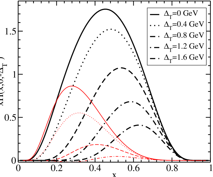
Figure 1: The generalized parton distributions $H_{u}(x,0,\Delta_{T}^{2})$ and $H_{d}(x,0,\Delta_{T}^{2})$ for the proton in the light-cone diquark model as functions of x for different values of $\Delta_{T}$.

The quark OAM distribution $L_{q}(x)$ can then be defined as the expectation value of operator

$$\hat{O}_{L}=\int d\eta\textrm{e}^{-ixP^{+}\eta}\psi_{q}^{\dagger}(\vec{r}\times i\vec{D})^{z}\psi_{q},$$ (8)

between the proton state $|P\,S\rangle$:

$$L_{q}^{z}(x)=\left\langle P\,S\left|\hat{O}_{L}\right|P\,S\right\rangle$$ (9)

The quark OAM distribution can be obtained from ji97 ; Hoodbhoy:1998yb

$$L_{q}^{z}(x)=\frac{1}{2}\left\{x\left[H_{q}(x,0,0)+E_{q}(x,0,0)\right]-\widetilde{H}_{q}(x,0,0)\right\},$$ (10)

where $H_{q}(x,0,0)$, $\widetilde{H}_{q}(x,0,0)$ and $E_{q}(x,0,0)$ are the forward limits of GPDs. Furthermore, the former two are the unpolarized and helicity distributions for the nucleon, respectively,

$$q(x)=H_{q}(x,0,0),~{}~{}~{}~{}\Delta q(x)=\widetilde{H}_{q}(x,0,0),$$ (11)

and $E_{q}(x,0,0)$ is related to the anomalous magnetic momentum of the nucleon in the following way:

$$\int_{0}^{1}dxE_{q}(x,0,0)=\kappa_{q},$$ (12)

where $\kappa_{q}$ is the contribution of quark flavor $q$ to the nucleon anomalous magnetic momentum.

III GPDs in the light-cone diquark model from the overlap representation formalism

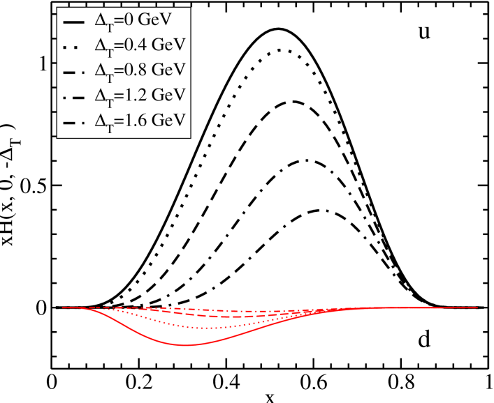
Figure 2: The generalized parton distributions $\widetilde{H}_{u}(x,0,\Delta_{T}^{2})$ and $\widetilde{H}_{d}(x,0,\Delta_{T}^{2})$ for the proton in the light-cone diquark model as functions of x for different values of $\Delta_{T}$.

In this section we present the calculation of the GPDs in the light-cone diquark model from the overlap representation formalism. The proton wave function with helicity $\Uparrow,\Downarrow$ in the SU(6) quark-diquark model ref:qdq ; Ma ; Ma:2002ir in the instant form is written as

$$\Psi^{\Uparrow,\Downarrow}(qD)=\frac{1}{\sqrt{2}}\varphi_{V}|qV\rangle^{\Uparrow,\Downarrow}+\frac{1}{\sqrt{2}}\varphi_{S}|qS\rangle^{\Uparrow,\Downarrow},$$ (13)

where $D=V,S$ denotes the vector diquark and scalar diquark, respectively. The

$$|qV\rangle^{\Uparrow,\Downarrow} = \pm\frac{1}{3}[V_{0}(ud)u^{\uparrow,\downarrow}-\sqrt{2}V_{\pm 1}(ud)u^{\downarrow,\uparrow}$$

$$-\sqrt{2}V_{0}(uu)d^{\uparrow,\downarrow}+2V_{\pm 1}(uu)d^{\downarrow,\uparrow}];$$

$$|qS\rangle^{\Uparrow,\Downarrow} = S(ud)u^{\uparrow,\downarrow},$$ (14)

The spin part of the light-cone wave function of the proton can be obtained from the instant form of the wave function by a Melosh rotation. For a spin-$\frac{1}{2}$ particle, the Melosh transformations are known to be ref:melosh

$$\chi^{\uparrow}_{T} = \omega\left[\left(k^{+}+m_{q}\right)\chi^{\uparrow}_{F}-k^{R}\chi^{\downarrow}_{F}\right],$$

$$\chi^{\downarrow}_{T} = \omega\left[\left(k^{+}+m_{q}\right)\chi^{\downarrow}_{F}+k^{L}\chi^{\uparrow}_{F}\right],$$ (15)

where $\chi_{T}$ and $\chi_{F}$ are instant and light-cone spinors respectively, $\omega=\left[2k^{+}\left(k^{0}+m_{q}\right)\right]^{-\frac{1}{2}}$, $k^{R,L}=k^{1}\pm ik^{2}$, and $m_{q}$ is the quark mass. In this work, for simplicity we treat the diquark as a point particle. The scalar diquark does not transform, since it has zero spin. For the spin-$1$ vector diquark, the Melosh transformations are given by ref:as

$$V^{1}_{T} = \omega_{V}^{2}\left[\left(k_{V}^{+}+\lambda_{V}\right)^{2}V^{1}_{F}-\sqrt{2}\left(k_{V}^{+}+\lambda_{V}\right)k_{V}^{R}V^{0}_{F}+{k_{V}^{R}}^{2}V^{-1}_{F}\right],$$

$$V^{0}_{T} = \omega_{V}^{2}\left[\sqrt{2}\left(k_{V}^{+}+\lambda_{V}\right)k_{V}^{L}V^{1}_{F}+2\left(\left(k_{V}^{0}+\lambda_{V}\right)k_{V}^{+}-k_{V}^{R}k_{V}^{L}\right)V^{0}_{F}\right.$$ (16)

$$-\sqrt{2}\left.\left(k_{V}^{+}+\lambda_{V}\right)k_{V}^{R}V^{-1}_{F}\right],$$

$$V^{-1}_{T} = \omega_{V}^{2}\left[{k_{V}^{L}}^{2}V^{1}_{F}+\sqrt{2}\left(k_{V}^{+}+\lambda_{V}\right)k_{V}^{L}V^{0}_{F}+\left(k_{V}^{+}+\lambda_{V}\right)^{2}V^{-1}_{F}\right].$$

Here, $\lambda_{V}$ denotes the mass of the diquark, $V_{T}$ and $V_{F}$ are the instant and light-cone spin-$1$ particle respectively, which are constructed within the Weinberg-Soper formalism weinberg64 .

After some algebra we arrive at the two body light-cone wavefunctions of the proton with

$$\Psi_{F}^{\uparrow,\downarrow}=\frac{1}{\sqrt{2}}|u\,S\rangle_{F}^{\Uparrow,\Downarrow}+\frac{1}{\sqrt{6}}|u\,V\rangle_{F}^{\Uparrow,\Downarrow}-\frac{1}{\sqrt{3}}|d\,V\rangle_{F}^{\Uparrow,\Downarrow}.$$ (17)

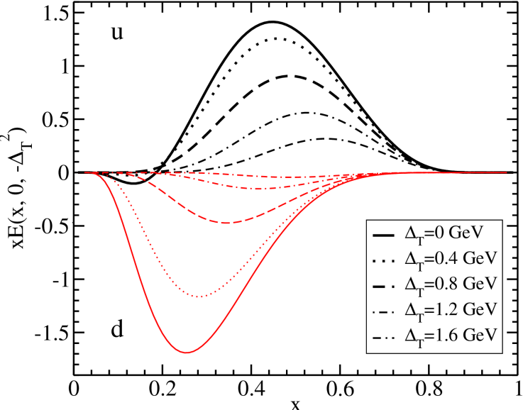
Figure 3: The generalized parton distributions $E_{u}(x,0,\Delta_{T}^{2})$ and $E_{d}(x,0,\Delta_{T}^{2})$ for the proton in the light-cone diquark model as functions of x for different values of $\Delta_{T}$.

The scalar diquark component of the wavefunction for the proton has the form

$$|u\,S(P^{+},\bm{k}_{T})\rangle^{\Uparrow,\Downarrow} = \sum_{s_{z}=\pm\frac{1}{2}}\int\frac{d^{2}\bm{k}_{T}dx}{\sqrt{x(1-x)}16\pi^{3}}$$ (18)

$$\times \psi^{\Uparrow,\Downarrow}_{S}(x,\bm{k}_{T},s_{z})|xP^{+},\bm{k}_{T},s_{z}\rangle,$$

while the vector diquark component is expressed as

$$|q\,V(P^{+},\bm{k}_{T})\rangle^{\Uparrow,\Downarrow} = \sum_{l_{z}=0,\pm 1;\,s_{z}=\pm\frac{1}{2}}\int\frac{d^{2}\bm{k}_{T}dx}{\sqrt{x(1-x)}16\pi^{3}}$$ (19)

$$\times \psi^{\Uparrow,\Downarrow}_{V}(x,\bm{k}_{T},l_{z},s_{z})|xP^{+},\bm{k}_{T},l_{z},s_{z}\rangle,$$

which is the same for $|u\,V\rangle_{F}$ and $|d\,V\rangle_{F}$. Here we denote $s_{z}$ and $l_{z}$ as the spin projections of the quark and the vector diquark. The forms of $\psi^{\Uparrow,\Downarrow}_{S}(x,\bm{k}_{T},s_{z})$ and $\psi^{\Uparrow,\Downarrow}_{V}(x,\bm{k}_{T},l_{z},s_{z})$ are given in the appendix.

Now we calculate the chiral-even GPDs in the zero skewedness ($\xi=0$) where $t=-\bm{\Delta_{T}}^{2}$. In the overlap representation Diehl:2000xz ; Brodsky:2000xy $H$, $E$ and $\widetilde{H}$ at $\xi=0$ can be expressed in a symmetric frame as ( in the domain $0<x<1$ and for $n\rightarrow n$ transition):

$$H(x,0,-\bm{\Delta}_{T}^{2}) = \sum_{n,\lambda_{i}}\int\prod_{i=1}^{n}\frac{dx_{i}d^{2}\bm{k}_{Ti}}{16\pi^{3}}16\pi^{3}\delta\left(1-\sum_{j=1}^{n}x_{j}\right)\delta^{(2)}\left(\sum_{j=1}^{n}\bm{k}_{Tj}\right)\delta(x-x_{1})\psi_{n}^{\uparrow\star}(x_{i}^{\prime},\bm{k}_{Ti}^{\prime},\lambda_{i})\psi_{n}^{\uparrow}(y_{i},\bm{l}_{Ti},\lambda_{i}),$$ (20)

$$\frac{\bm{\Delta}_{L}}{2M}E(x,0,-\bm{\Delta}_{T}^{2}) = \sum_{n,\lambda_{i}}\int\prod_{i=1}^{n}\frac{dx_{i}d^{2}\bm{k}_{Ti}}{16\pi^{3}}16\pi^{3}\delta\left(1-\sum_{j=1}^{n}x_{j}\right)\delta^{(2)}\left(\sum_{j=1}^{n}\bm{k}_{Tj}\right)\delta(x-x_{1})\psi_{n}^{\uparrow\star}(x_{i}^{\prime},\bm{k}_{Ti}^{\prime},\lambda_{i})\psi_{n}^{\downarrow}(y_{i},\bm{l}_{Ti},\lambda_{i}),$$ (21)

$$\widetilde{H}(x,0,-\bm{\Delta}_{T}^{2}) = \sum_{n,\lambda_{i}}\int\prod_{i=1}^{n}\textrm{sign}(\lambda_{i})\frac{dx_{i}d^{2}\bm{k}_{Ti}}{16\pi^{3}}16\pi^{3}\delta\left(1-\sum_{j=1}^{n}x_{j}\right)\delta^{(2)}\left(\sum_{j=1}^{n}\bm{k}_{Tj}\right)\delta(x-x_{1})\psi_{n}^{\uparrow\star}(x_{i}^{\prime},\bm{k}_{Ti}^{\prime},\lambda_{i})\psi_{n}^{\uparrow}(y_{i},\bm{l}_{Ti},\lambda_{i}),$$

with

$$x^{\prime}_{1} = x_{1},~{}~{}~{}~{}~{}~{}\bm{k}_{T1}^{\,\prime}=\bm{k}_{T1}-(1-x_{1})\frac{\bm{\Delta_{T}}}{2}$$

for the final struck quark,

$$x^{\prime}_{i} = x_{i},~{}~{}~{}~{}~{}~{}~{}\bm{k}_{Ti}^{\,\prime}=\bm{k}_{Ti}+x_{i}\frac{\bm{\Delta_{T}}}{2}$$

for the final (n-1) spectators,

and

$$y_{1} = x_{1},~{}~{}~{}~{}~{}~{}\bm{l}_{T1}^{\,\prime}=\bm{k}_{T1}+(1-x_{1})\frac{\bm{\Delta_{T}}}{2}$$

for the initial struck quark,

$$y_{i} = x_{i},~{}~{}~{}~{}~{}~{}~{}\bm{l}_{Ti}=\bm{k}_{Ti}-x_{i}\frac{\bm{\Delta_{T}}}{2}$$

for the initial (n-1) spectators,

From Eq. (21) we see that non-zero $E_{q}$ needs a spin flip between the initial and final proton wavefunctions. The same kind of overlap integration of light-front wavefunctions (with $J_{z}=\pm 1/2$ in the initial and final states) also appears in the calculation ref:bhs of Sivers functions, which indicates the presence of the quark OAM .

By employing the light-cone wavefunctions given in (17) and the overlap representation formalism, we calculate the generalized parton distribution functions (GPDs) $H_{q}(x,0,-\bm{\Delta}_{T}^{2})$, $\widetilde{H}_{q}(x,0,-\bm{\Delta}_{T}^{2})$ and $E_{q}(x,0,-\bm{\Delta}_{T}^{2})$ at zero skewedness for $q=u$ and $d$ quarks. The $x$-dependence of these GPDs at different values of $\Delta_{T}$ are given in Figs. 1, 2 and 3, respectively.

From Fig. 3 one can see that $E_{u}$ and $E_{d}$ have opposite sign ($E_{u}$ is positive and $E_{d}$ is negative) with similar size in our model. Since it has been shown that there is a quantitative relation amm ; ls07 ; gpdtmd between the Sivers function $f_{1T}^{\bot q}$ and the GPD $E^{q}$, our result coincides with recent extractions Anselmino:2005ea ; Efremov:2004tp ; Vogelsang:2005cs of the Sivers function from the Semi-inclusive deeply inelastic scattering data, which show the Sivers functions of $u$ and $d$ have opposite sign with similar size.

Special attention should be paid to the limit of zero momentum transfer $\Delta_{T}^{2}=0$, since in this limit the GPDs $H_{q}$ and $\widetilde{H}_{q}$ are simplified to the forward distribution $q(x)$ and $\Delta_{q}(x)$. Also the quark OAM s are related in the way shown in (11), from which in principle one can calculates $L_{q}(x)$ from the known chiral-even GPDs.

By taking the GPDs in the forward limit, we calculate the OAM distributions of u and d quarks inside the proton, as shown in Fig. 4. It can be seen that in our model $L_{u}(x)$ is positive, while $L_{d}(x)$ is consistent with zero compared with $L_{u}(x)$, and the net OAM of the $u$ and $d$ quarks is positive. From Fig. 3 one can see that $E_{d}$ is sizable. However, since $E_{d}$ is negative, there is a cancelation between $d(x)$, $E_{d}(x)$ and $\Delta q(x)$. This leads to a small contribution of the $d$ quark orbital angular momentum. We remind that there are Lattice QCD Hagler:2003jd ; Gockeler:2003jfa , as well as phenomenological parametrizations and other model calculations of GPDs  Ossmann:2004bp ; Guidal:2004nd ; Diehl:2004cx ; Wakamatsu:2005vk ; Wakamatsu:2006dy , which are used to estimate the OAM of the quarks.

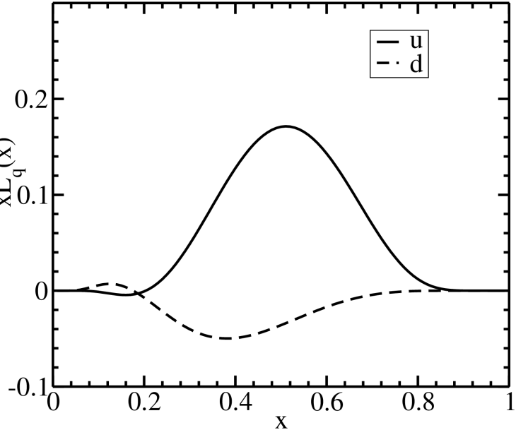
Figure 4: The OAM distributions $L_{q}(x)$ of $u$ and $d$ quarks inside the proton in the light-cone diquark model as functions of $x$.

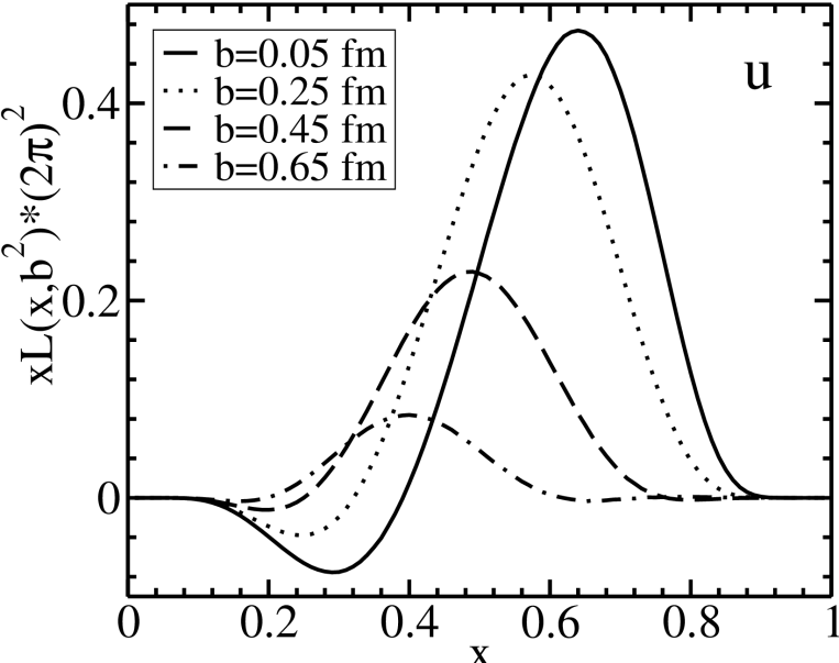
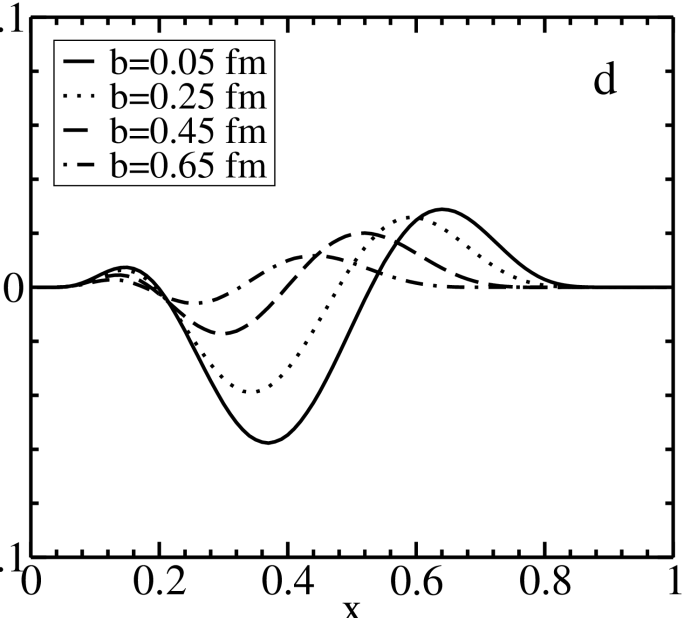
Figure 5: The impact parameter distributions (scaled with a factor of $(2\pi)^{2}$) $xL_{u}(x,\bm{b}_{T})$ (left) and $xL_{d}(x,\bm{b}_{T})$ (right) for the proton in the light-cone diquark model as functions of $x$ for different values of $b$.

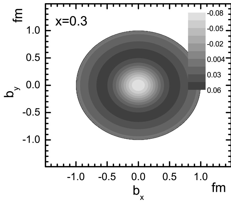
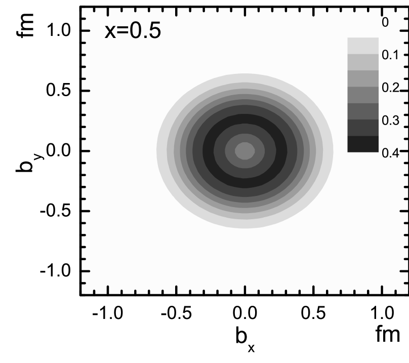
Figure 6: The profiles of the impact parameter distribution (scaled by a factor of $(2\pi)^{2}$) $xL_{u}(x,\bm{b}_{T})$ for the proton in the light-cone diquark model as functions of $\Delta_{T}$ for $x=0.3$ (left) and $x=0.5$ (right).

IV Impact parameter dependence of Orbital angular momentum

In this section we want to study the quark OAM s in transverse position (impact parameter) space. The GPDs in the impact parameter space have been studied in Refs. Burkardt:2000za ; Diehl:2002he ; Burkardt:2002hr . The most interesting case is the zero skewedness limit $\xi=0$, in which a density interpretation of GPDs in the impact parameter space may be obtained Burkardt:2000za , Therefore studying GPDs in impact parameter space can provide a three-dimensional picture of the nucleon. In the following we restrict ourselves to the case $\xi=0$.

The impact parameter PDFs inside the nucleon can be obtained by sandwiching the parton correlator between nucleon states localized in transverse space

$$q(x,\bm{b}_{T}) = \;\big{<}P^{+},\bm{0}_{T};S\big{|}\hat{\mathcal{O}}^{[\gamma^{+}]}_{q}(x,\bm{b}_{T})\big{|}P^{+},\bm{0}_{T};S\big{>},$$ (23)

where

$$\hat{{O}}^{[\gamma^{+}]}_{q}(x,\bm{b}_{T})$$ (24)

$$= \int\frac{dy^{-}}{8\pi}\;e^{ixP^{+}y^{-}/2}\;\bar{\psi}(0,-\frac{y^{-}}{2},\bm{b}_{T})\,\gamma^{+}\,\psi(0,\frac{y^{-}}{2},\bm{b}_{T}),$$

and the initial and final states in the transverse space defined as  Soper:1976jc ; Burkardt:2000za ; Diehl:2002he

$$\big{|}P^{+},\bm{b}_{T};S\big{>} =\mathcal{N}\int\frac{d^{2}\bm{p}_{T}}{(2\pi)^{2}}\,e^{-i\bm{p}_{T}\cdot\bm{b}_{T}}\,\big{|}p;S\big{>}\,,$$ (25)

$$\big{<}P^{+},\bm{b}_{T};S\big{|} =\mathcal{N^{*}}\int\frac{d^{2}{\bm{p}\,}^{\prime}_{\!T}}{(2\pi)^{2}}\,e^{i{\bm{p}\,}^{\prime}_{\!T}\cdot\bm{b}_{T}}\,\big{<}p^{\prime};S\big{|}\,,$$ (26)

which characterize a nucleon with momentum $P^{+}$ at a transverse position $\bm{b}_{T}$ and polarization specified by $S$.

One of the interesting features of impact parameter dependent parton distributions is that they are Fourier transformations of GPDs Burkardt:2000za . For instance, The impact parameter dependence of unpolarized quark in the unpolarized nucleon can be obtained from

$$q(x,\bm{b}_{T})=\int\frac{d^{2}\bm{\Delta}_{T}}{(2\pi)^{2}}e^{-i\bm{b}_{T}\cdot\bm{\Delta}_{T}}H_{q}(x,0,-\bm{\Delta}_{T}^{2}),$$ (27)

here $\bm{b}_{T}$ and $\bm{\Delta}_{T}$ are two conjugated parameters.

Similarly the impact parameter dependence of quark helicity distribution in the longitudinal polarized nucleon is defined as

$$\Delta q(x,\bm{b}_{T}) = \;\big{<}P^{+},\bm{0}_{T};S\big{|}\hat{\mathcal{O}}^{[\gamma^{+}\gamma_{5}]}_{q}(x,\bm{b}_{T})\big{|}P^{+},\bm{0}_{T};S\big{>},$$ (28)

Which is the Fourier transformation of $\widetilde{H}_{q}$:

$$q(x,\bm{b}_{T})=\int\frac{d^{2}\bm{\Delta}_{T}}{(2\pi)^{2}}e^{-i\bm{b}_{T}\cdot\bm{\Delta}_{T}}H_{q}(x,0,-\bm{\Delta}_{T}^{2}),$$ (29)

We follow a similar approach by introducing the impact parameter dependence of quark OAM $\mathcal{L}(x,\bm{b}_{T})$. It can be obtained from the expectation value of $\hat{O}_{L}$, given in Eq. (8), between the position state $|P^{+},\bm{0}_{T}\rangle$:

$$L_{q}(x,\bm{b}_{T})=\left\langle P,\bm{0}_{T};S\left|\hat{O}_{L}\right|P,\bm{0}_{T};S\right\rangle$$ (30)

After a Fourier transformation on $L_{q}(x,\bm{b}_{T})$ one can arrive at

$$\int d^{2}\bm{b}_{T}\,\textrm{e}^{\textrm{i}\bm{b}_{T}\,\cdot\,\bm{\Delta}_{T}}\,L_{q}^{z}(x,\bm{b}_{T})=L_{q}(x,-\bm{\Delta}^{2}_{T})$$ (31)

The function $L_{q}^{z}(x,-\bm{\Delta}^{2}_{T})$ can be obtained by the GPDs at zero skewedness ji97

$$L_{q}(x,-\bm{\Delta}^{2}_{T}) = \frac{1}{2}\left\{x\left[H(x,0,-\bm{\Delta}^{2}_{T})+E_{q}(x,0,-\bm{\Delta}^{2}_{T})\right]\right.$$ (32)

$$- \left.\widetilde{H}(x,0,-\bm{\Delta}^{2}_{T})\right\},$$

and (11) is the forward limit of $L_{q}(x,-\bm{\Delta}^{2}_{T})$.

Therefore, if we know the GPDs $H_{q}$ $\widetilde{H}_{q}$ and $E_{q}$, from (11) one can calculate the impact parameter dependence of the quark OAM distribution by the Fourier transformation

$$L_{q}(x,\bm{b}_{T})=\int{d^{2}\bm{\Delta}_{T}\over(2\pi)^{2}}\,\textrm{e}^{-\textrm{i}\bm{b}_{T}\,\cdot\,\bm{\Delta}_{T}}\,L_{q}^{z}(x,\bm{\Delta}^{2}_{T}).$$ (33)

The integration over impact parameter dependence of quark OAM leads to

$$\int d^{2}\bm{b}_{T}L_{q}(x,\bm{b}_{T})=L_{q}(x)$$ (34)

In Fig. 5 we shown the impact parameter distributions (scaled with a factor of $(2\pi)^{2}$) $L_{u}(x,\bm{b}_{T})$ (left) and $L_{d}(x,\bm{b}_{T})$ (right) for the proton in the light-cone diquark model, as functions of $x$, for different values of $b$. In Fig. 6 we show the profiles of the impact parameter distributions $L_{u}(x,\bm{b}_{T})$ for the proton in the light-cone diquark model as functions of $\bm{b}_{T}$, for $x=0.3$ and $x=0.5$. It is shown that the impact parameter dependence of quark OAM is axially symmetric. Also at large $x$ the impact parameter distribution is peaked at small $b$.

V summary

As a conclusion, we study the OAM structure of the quarks inside the proton in a light-cone diquark model. In this model the light-cone wave function of the proton is known. It is then convenient to express the physical observables in the overlap representation formalism. We calculate the chiral-even generalized parton distribution functions (GPDs) $H_{q}(x,\xi,\Delta^{2})$, $\widetilde{H}_{q}(x,\xi,\Delta^{2})$ and $E_{q}(x,\xi,\Delta^{2})$ at zero skewedness for $q=u$ and $d$. We found that $E_{u}$ and $E_{d}$ have opposite sign, with similar size in our model. The GPDs are applied to calculate the OAM distributions, showing that $L_{u}(x)$ is positive, while $L_{d}(x)$ is consistent with zero compared with $L_{u}(x)$, and the net OAM of the $u$ and $d$ quarks is positive. We also introduce the impact parameter dependence of quark OAM distribution $L(x,\bm{b}_{T})$ . It describes the position space distribution of the quark OAM at given $x$. We found that the impact parameter dependence of quark OAM distribution is axially symmetric in the light-cone diquark model.

Appendix A light-cone wave functions in a diquark model

The expressions for $\psi^{\Uparrow,\Downarrow}_{S}(x,\bm{k}_{T},s_{z})$ have the form

$$\psi^{\Uparrow}_{S}(x,\bm{k}_{T},+\frac{1}{2}) = \frac{(k^{+}+m)}{\omega}\phi_{S}(x,k_{T}),$$

$$\psi^{\Uparrow}_{S}(x,\bm{k}_{T},-\frac{1}{2}) = -\frac{k_{r}}{\omega}\phi_{S}(x,k_{T}),$$ (35)

and

$$\psi^{\Downarrow}_{S}(x,\bm{k}_{T},+\frac{1}{2}) = \frac{k_{l}}{\omega}\phi_{S}(x,k_{T}),$$

$$\psi^{\Downarrow}_{S}(x,\bm{k}_{T},-\frac{1}{2}) = \frac{(k^{+}+m)}{\omega}\phi_{S}(x,k_{T}),$$ (36)

respectively.

The expressions of $\psi^{\Uparrow,\Downarrow}_{V}(x,\bm{k}_{T},l_{z},s_{z})$ can be expressed as

$$\psi^{\Uparrow}_{V}(x,\bm{k}_{T},+1,\uparrow) = -\sqrt{2}\frac{\phi_{V}(x,k_{T})}{\omega\omega^{2}_{V}}\bigg{[}(k_{V}^{+}+\lambda_{V})(k^{+}+m)$$

$$+(k_{V}^{+}+\lambda_{V})^{2}\bigg{]}k^{L},$$

$$\psi^{\Uparrow}_{V}(x,\bm{k}_{T},+1,\downarrow) = \sqrt{2}\frac{\phi_{V}(x,k_{T})}{\omega\omega^{2}_{V}}\bigg{[}(k_{V}^{+}+\lambda_{V})\bm{k}_{T}^{2}$$

$$-(k_{V}^{+}+\lambda_{V})^{2}(k^{+}+m)\bigg{]},$$

$$\psi^{\Uparrow}_{V}(x,\bm{k}_{T},0,\uparrow) = 2\frac{\phi_{V}(x,k_{T})}{\omega\omega^{2}_{V}}\left\{\bigg{[}(k_{V}^{0}+\lambda_{V})k_{V}^{+}-\bm{k}_{T}^{2}\bigg{]}(k^{+}+m)\right.$$ (37)

$$\left.-(k_{V}^{+}+\lambda_{V})\bm{k}_{T}^{2}\right\},$$

$$\psi^{\Uparrow}_{V}(x,\bm{k}_{T},0,\downarrow) = \frac{\phi_{V}(x,k_{T})}{\omega\omega^{2}_{V}}\bigg{[}-2((k_{V}^{0}+\lambda_{V})k_{V}^{+}-\bm{k}_{T}^{2})$$

$$-2(k_{V}^{+}+\lambda_{V})(k^{+}+m)\bigg{]}k^{R},$$

$$\psi^{\Uparrow}_{V}(x,\bm{k}_{T},-1,\uparrow) = \sqrt{2}\frac{\phi_{V}(x,k_{T})}{\omega\omega^{2}_{V}}\bigg{[}(k_{V}^{+}+\lambda_{V})(k^{+}+m)-\bm{k}_{T}^{2}\bigg{]}k^{R},$$

$$\psi^{\Uparrow}_{V}(x,\bm{k}_{T},-1,\downarrow) = -\sqrt{2}\frac{\phi_{V}(x,k_{T})}{\omega\omega^{2}_{V}}\bigg{[}k^{R2}_{T}(k_{V}^{+}+\lambda_{V}+k^{+}+m)\bigg{]},$$

and

$$\psi^{\Downarrow}_{V}(x,\bm{k}_{T},+1,\uparrow) = -\sqrt{2}\frac{\phi_{V}(x,k_{T})}{\omega\omega^{2}_{V}}\bigg{[}k^{L2}_{T}(k_{V}^{+}+\lambda_{V}+k^{+}+m)\bigg{]},$$

$$\psi^{\Downarrow}_{V}(x,\bm{k}_{T},+1,\downarrow) = -\sqrt{2}\frac{\phi_{V}(x,k_{T})}{\omega\omega^{2}_{V}}\bigg{[}(k_{V}^{+}+\lambda_{V})(k^{+}+m)$$

$$-\bm{k}_{T}^{2}\bigg{]}k^{L},$$

$$\psi^{\Downarrow}_{V}(x,\bm{k}_{T},0,\uparrow) = 2\frac{\phi_{V}(x,k_{T})}{\omega\omega^{2}_{V}}\bigg{[}((k_{V}^{0}+\lambda_{V})k_{V}^{+}-\bm{k}_{T}^{2})$$ (38)

$$+(k_{V}^{+}+\lambda_{V})(k^{+}+m)\bigg{]}k^{L},$$

$$\psi^{\Downarrow}_{V}(x,\bm{k}_{T},0,\downarrow) = 2\frac{\phi_{V}(x,k_{T})}{\omega\omega^{2}_{V}}\left\{\bigg{[}(k_{V}^{0}+\lambda_{V})k_{V}^{+}-\bm{k}_{T}^{2}\bigg{]}(k^{+}+m)\right.$$

$$-\left.(k_{V}^{+}+\lambda_{V})\bm{k}_{T}^{2}\right\},$$

$$\psi^{\Downarrow}_{V}(x,\bm{k}_{T},-1,\uparrow) = \sqrt{2}\frac{\phi_{V}(x,k_{T})}{\omega\omega^{2}_{V}}\bigg{[}(k_{V}^{+}+\lambda_{V})\bm{k}_{T}^{2}$$

$$-(k_{V}^{+}+\lambda_{V})^{2}(k^{+}+m)\bigg{]},$$

$$\psi^{\Downarrow}_{V}(x,\bm{k}_{T},-1,\downarrow) = \sqrt{2}\frac{\phi_{V}(x,k_{T})}{\omega\omega^{2}_{V}}\bigg{[}(k_{V}^{+}+\lambda_{V})(k^{+}+m)$$

$$+(k_{V}^{+}+\lambda_{V})^{2}\bigg{]}k^{R},$$

The momentum dependence of the wavefunctions in the above equations is described by $\phi_{D}(x,k_{T}^{2})$ with the Gaussian form

$$\phi_{D}(x,k_{T})=A_{D}\exp\left(-\frac{\mathcal{M}^{2}}{8\beta_{D}^{2}}\right),$$ (39)

where

$$\mathcal{M}^{2}=\frac{\bm{k}_{T}^{2}+m_{q}^{2}}{x}+\frac{\bm{k}_{T}^{2}+\lambda_{V}^{2}}{1-x},$$ (40)

$A_{D}$ stands for the normalization constant, and $\beta_{D}$ is the oscillation factor. For the parameters we adopt the values from Ma:2002ir , which can describe the data of the nucleon form factors.

References

• (1) EMC Collaboration, J. Ashman et al.,Phys.Lett. B202 (1988) 603; Nucl. Phys. B 328 (1989) 1.
• (2) L. M. Sehgal, Phys. Rev.  D 10, 1663 (1974) [Erratum-ibid.  D 11, 2016 (1975)].
• (3) R. L. Jaffe and A. Manohar, Nucl. Phys. B 337 (1990) 509.
• (4) X. Ji, Phys. Rev. Lett. 78 (1997) 610.
• (5) P. Hagler and A. Schafer, Phys. Lett. B 430 (1998) 179.
• (6) A. Harindranath and R. Kundu, Phys. Rev. D 59 (1999) 116013.
• (7) B. Q. Ma and I. Schmidt, Phys. Rev.  D 58, 096008 (1998) [arXiv:hep-ph/9808202].
• (8) D. Mueller, D. Robaschik, B. Geyer, F. M. Dittes and J. Horejsi, Fortsch. Phys.  42, 101 (1994) [arXiv:hep-ph/9812448].
• (9) X. D. Ji, Phys. Rev.  D 55, 7114 (1997) [arXiv:hep-ph/9609381].
• (10) A. V. Radyushkin, Phys. Rev.  D 56, 5524 (1997) [arXiv:hep-ph/9704207].
• (11) M. Diehl, Phys. Rept. 388 (2003) 41.
• (12) A. V. Belitsky and A. V. Radyushkin, Phys. Rept.  418, 1 (2005) [arXiv:hep-ph/0504030].
• (13) S. Boffi and B. Pasquini, Riv. Nuovo Cim.  30, 387 (2007) [arXiv:0711.2625 [hep-ph]].
• (14) A. V. Radyushkin, Phys. Lett.  B 380, 417 (1996) [arXiv:hep-ph/9604317].
• (15) M. V. Polyakov, Nucl. Phys.  B 555, 231 (1999) [arXiv:hep-ph/9809483].
• (16) J. C. Collins, L. Frankfurt and M. Strikman, Phys. Rev.  D 56, 2982 (1997) [arXiv:hep-ph/9611433].
• (17) P. J. Mulders and R. D. Tangerman, Nucl. Phys.  B 461, 197 (1996) [Erratum-ibid.  B 484, 538 (1997)] [arXiv:hep-ph/9510301].
• (18) D. Boer and P. J. Mulders, Phys. Rev.  D 57, 5780 (1998) [arXiv:hep-ph/9711485].
• (19) D. W. Sivers, Phys. Rev.  D 41, 83 (1990).
• (20) D. W. Sivers, Phys. Rev.  D 43, 261 (1991).
• (21) A. Airapetian et al. (HERMES Collaboration), Phys. Rev. Lett. 94, 012002 (2005).
• (22) M. Diefenthaler [HERMES Collaboration], AIP Conf. Proc.  792, 933 (2005) [arXiv:hep-ex/0507013].
• (23) V.Yu. Alexakhin et al. (COMPASS Collaboration), Phys. Rev. Lett. 94, 202002 (2005).
• (24) E. S. Ageev et al. [COMPASS Collaboration], Nucl. Phys.  B 765, 31 (2007) [arXiv:hep-ex/0610068].
• (25) M. Burkardt and D. S. Hwang, Phys. Rev. D 69, 074032 (2004); M. Burkardt, ibid. D 72, 094020 (2005);
• (26) M. Burkardt and G. Schnell, Phys. Rev.  D 74, 013002 (2006) [arXiv:hep-ph/0510249].
• (27) Z. Lu and I. Schmidt, Phys. Rev.  D 75, 073008 (2007) [arXiv:hep-ph/0611158].
• (28) M. Diehl and Ph. Hagler, Eur. Phys. J.  C 44, 87 (2005) [arXiv:hep-ph/0504175].
• (29) M. Gockeler et al. [QCDSF Collaboration and UKQCD Collaboration], Phys. Rev. Lett.  98, 222001 (2007) [arXiv:hep-lat/0612032].
• (30) S. Meissner, A. Metz, and K. Goeke, Phys. Rev. D 76, 034002 (2007).
• (31) S. Meissner, A. Metz, M. Schlegel and K. Goeke, JHEP 0808, 038 (2008) [arXiv:0805.3165 [hep-ph]].
• (32) S. Meissner, A. Metz and M. Schlegel, JHEP 0908, 056 (2009) [arXiv:0906.5323 [hep-ph]].
• (33) M. Burkardt, Phys. Rev.  D 66, 114005 (2002) [arXiv:hep-ph/0209179].
• (34) M. Burkardt, Nucl. Phys.  A 735, 185 (2004) [arXiv:hep-ph/0302144].
• (35) M. Burkardt, Phys. Rev.  D 62, 071503 (2000) [Erratum-ibid.  D 66, 119903 (2002)] [arXiv:hep-ph/0005108].
• (36) M. Burkardt, Int. J. Mod. Phys.  A 18, 173 (2003) [arXiv:hep-ph/0207047].
• (37) M. Diehl, Eur. Phys. J.  C 25, 223 (2002) [Erratum-ibid.  C 31, 277 (2003)] [arXiv:hep-ph/0205208].
• (38) M. Burkardt and D. S. Hwang, Phys. Rev.  D 69, 074032 (2004) [arXiv:hep-ph/0309072].
• (39) S. J. Brodsky, M. Diehl and D. S. Hwang, Nucl. Phys.  B 596, 99 (2001) [arXiv:hep-ph/0009254].
• (40) M. Diehl, T. Feldmann, R. Jakob and P. Kroll, Nucl. Phys.  B 596, 33 (2001) [Erratum-ibid.  B 605, 647 (2001)] [arXiv:hep-ph/0009255].
• (41) M. Burkardt and B. C. Hikmat, Phys. Rev.  D 79, 071501 (2009) [arXiv:0812.1605 [hep-ph]].
• (42) P. Hoodbhoy, X. D. Ji and W. Lu, Phys. Rev.  D 59, 014013 (1999) [arXiv:hep-ph/9804337].
• (43) M.I. Pavkovi$\acute{\textmd{c}}$, Phys. Rev. D 13 (1976) 2128.
• (44) B. Q. Ma, Phys. Lett.  B 375, 320 (1996) [Erratum-ibid.  B 380, 494 (1996)] [arXiv:hep-ph/9604423].
• (45) B. Q. Ma, D. Qing and I. Schmidt, Phys. Rev.  C 65, 035205 (2002) [arXiv:hep-ph/0202015].
• (46) H.J. Melosh, Phys. Rev. D 9 (1974) 1095.
• (47) D.V. Ahluwalia and M. Sawicki, Phys. Rev. D 47 (1993) 5161.
• (48) S. Weinberg, Phys. Rev. B133, 1318 (1964); D. E. Soper, Ph.D. thesis, SLAC (1971).
• (49) S.J. Brodsky, D.S. Hwang, and I. Schmidt, Phys. Lett. B 530 (2002) 99.
• (50) M. Anselmino, M. Boglione, U. D’Alesio, A. Kotzinian, F. Murgia and A. Prokudin, Phys. Rev.  D 72, 094007 (2005) [Erratum-ibid.  D 72, 099903 (2005)] [arXiv:hep-ph/0507181].
• (51) A. V. Efremov, K. Goeke, S. Menzel, A. Metz and P. Schweitzer, Phys. Lett.  B 612, 233 (2005) [arXiv:hep-ph/0412353].
• (52) W. Vogelsang and F. Yuan, Phys. Rev.  D 72, 054028 (2005) [arXiv:hep-ph/0507266].
• (53) P. Hagler, J. W. Negele, D. B. Renner, W. Schroers, T. Lippert and K. Schilling [LHPC collaboration and SESAM collaboration], Phys. Rev.  D 68, 034505 (2003) [arXiv:hep-lat/0304018].
• (54) M. Gockeler, R. Horsley, D. Pleiter, P. E. L. Rakow, A. Schafer, G. Schierholz and W. Schroers [QCDSF Collaboration], Phys. Rev. Lett.  92, 042002 (2004) [arXiv:hep-ph/0304249].
• (55) J. Ossmann, M. V. Polyakov, P. Schweitzer, D. Urbano and K. Goeke, Phys. Rev.  D 71, 034011 (2005) [arXiv:hep-ph/0411172].
• (56) M. Guidal, M. V. Polyakov, A. V. Radyushkin and M. Vanderhaeghen, Phys. Rev.  D 72, 054013 (2005) [arXiv:hep-ph/0410251].
• (57) M. Diehl, T. Feldmann, R. Jakob and P. Kroll, Eur. Phys. J.  C 39, 1 (2005) [arXiv:hep-ph/0408173].
• (58) M. Wakamatsu and H. Tsujimoto, Phys. Rev.  D 71, 074001 (2005) [arXiv:hep-ph/0502030].
• (59) M. Wakamatsu and Y. Nakakoji, Phys. Rev.  D 74, 054006 (2006) [arXiv:hep-ph/0605279].
• (60) D. E. Soper, Phys. Rev.  D 15, 1141 (1977).