The probability distribution of a trapped Brownian particle in plane shear flows

Abstract

We investigate the statistical properties of an over-damped Brownian particle that is trapped by a harmonic potential and simultaneously exposed to a linear shear flow or to a plane Poiseuille flow. Its probability distribution is determined via the corresponding Smoluchowski equation, which is solved analytically for a linear shear flow. In the case of a plane Poiseuille flow, analytical approximations for the distribution are obtained by a perturbation analysis and are substantiated by numerical results. There is a good agreement between the two approaches for a wide range of parameters.

The dynamics of Brownian particles in fluids is of central importance in many areas of science Dhont:96 ; Berg:1993 . There is a profound understanding of Brownian motion in quiescent fluids, but the situation is different for particles in flows. Several statistical properties of free Brownian particles in open flows have been investigated, for instance, in terms of the corresponding Langevin and Fokker-Planck equations vdVen:1980.1 . Recent works also consider inertia effects on diffusion in shear flows Drossinos:05 ; Drossinos:2009.1 and the relation between the Gaussian nature of noise and time-reversibility in driven systems Rubi:2007.1 . It has also been shown that shear flow causes, compared to a quiescent fluid, additional correlations of the particle’s velocity and positional fluctuations Bedeaux:1995.1 ; Brady:04 ; Drossinos:05 . However, the detection of statistical properties of free particles in a flow is an intricate issue.

To overcome part of these problems, three recent works focused on the dynamics of Brownian particles trapped by harmonic potentials and exposed to shear flows Ziehl:2009.1 ; Holzer:2009.1 ; Bammert:2010.1 . It was shown that the shear-induced correlations between the positional fluctuations of a captured particle along orthogonal directions are essentially the same as in the free-particle case Holzer:2009.1 . Furthermore, a surprisingly good agreement was found between the predictions and the measurements of these correlations Ziehl:2009.1 .

In Ref. Holzer:2009.1 the probability distribution of a trapped Brownian particle in shear flows was obtained by simulations of the Langevin equation. In this brief report the related Smoluchowski equation for the probability distribution is presented and for a linear shear flow an exact analytical solution is given. For a plane Poiseuille flow we determine approximate analytical solutions, which are in good agreement for a wide parameter range with numerical solutions of the Smoluchowski equation and with simulations of the Langevin equation as well.

We consider a Brownian particle trapped by a harmonic potential with the spring constant $k$ at the origin of the Cartesian coordinate frame $({\bar{x}},{\bar{y}},{\bar{z}})$:

$$V(\mathbf{\bar{r}})=\frac{k}{2}\mathbf{\bar{r}}^{2}\,.$$ (1)

The particle is exposed to a flow along the ${\bar{x}}$-direction with a ${\bar{y}}$-dependent magnitude:

$$\mathbf{u}(\mathbf{\bar{r}})=(a+b\bar{y}+c\bar{y}^{2})\hat{\mathbf{e}}_{x}\,.$$ (2)

Since the Brownian motion perpendicular to the shear plane is decoupled from the one in the shear plane, we consider the quasi two-dimensional problem with $\mathbf{\bar{r}}=(\bar{x},\bar{y})$ and $\bar{\nabla}=(\partial_{\bar{x}},\partial_{\bar{y}})$.

For a plane Poiseuille flow the position of the potential minimum can be different from the center of the flow. In the shifted coordinate frame, $({\tilde{x}},{\tilde{y}})=({\bar{x}},{\bar{y}}+\tilde{y}_{0})$, where $\tilde{y}_{0}$ describes the $y$-coordinate of the potential minimum, the flow profile is given by $\mathbf{u}({\tilde{y}})=u_{p}(1-\tilde{y}^{2}/l^{2})\hat{\mathbf{e}}_{x}$ with the flow velocity $u_{p}$ at its center and the confining plane boundaries at $\tilde{y}=\pm l$. If a particle is trapped at $\tilde{y}_{0}\not=0$, one obtains with $\tilde{y}=\tilde{y}_{0}+\bar{y}$ the coefficients $a=u_{p}(1-\tilde{y}_{0}^{2}/l^{2})$, $b=-2u_{p}\tilde{y}_{0}/l^{2}$ and $c=-u_{p}/l^{2}$ in Eq. (2). This work focuses on situations where the particle positions are sufficiently far away from the boundaries, so that hydrodynamic interactions with the wall, as discussed in vdVen:1980.1 for instance, can be neglected.

The particle dynamics are determined by thermal motion, potential forces and drag forces caused by the flow. The thermal motion is characterized by the diffusion constant $D=k_{B}T/\zeta$, which is given by the Einstein relation in terms of the temperature $T$, the Boltzmann constant $k_{B}$ and the Stokes friction coefficient $\zeta=6\pi\eta R$, where $\eta$ is the viscosity of the fluid and $R$ is the effective radius of the particle. The external flow $\mathbf{u}$ is the origin of the Stokes drag force $\zeta\mathbf{u}$ on the point-like particle, which is balanced by the restoring force $-\bar{\nabla}V=-k\bar{\mathbf{r}}$.

The diffusion and the two deterministic forces drive the probability current $\mathbf{j}(x,y,t)$ of the Smoluchowski equation (SE) for the particle’s positional distribution function $\mathcal{P}(\bar{x},\bar{y},\bar{t})$ Risken:89 :

$$\partial_{\bar{t}}\mathcal{P} =-\bar{\nabla}\mathbf{j}\,,$$ (3)

$$\mathbf{j} =-D\bar{\nabla}\mathcal{P}+(\mathbf{u}-\frac{1}{\zeta}\nabla V)\mathcal{P}\,.$$ (4)

With the expressions in Eqs. (1) - (4) the SE of a Brownian particle trapped in a harmonic potential and exposed to a shear flow reads:

$$\partial_{\bar{t}}\mathcal{P}= D\bar{\nabla}^{2}\mathcal{P}+\frac{D}{\delta^{2}}\left(2+\bar{x}\partial_{\bar{x}}+\bar{y}\partial_{\bar{y}}\right)\mathcal{P}$$

$$-(a+b\bar{y}+c\bar{y}^{2})\partial_{\bar{x}}\mathcal{P}\,.$$ (5)

The two spatial coordinates may be rescaled by the length $\delta=\sqrt{k_{B}T/k}$, $\bar{x}=\delta x$ and $\bar{y}=\delta y$, alike the time, ${\bar{t}}=\zeta/k\,t$. This results in the dimensionless SE

$$\partial_{t}\mathcal{P}=\left[\nabla^{2}+2+y\partial_{y}+(x-\alpha-\beta y-\gamma y^{2})\partial_{x}\right]\mathcal{P}\,,$$ (6)

with the parameters $\alpha=a\delta/D$, $\beta=b\delta^{2}/D$ and $\gamma=c\delta^{3}/D$ describing the flow profile and $y\in[(-l-\tilde{y}_{0})/\delta,\,(l-\tilde{y}_{0})/\delta]$. $\beta$ is the so-called Weissenberg number. We note here, that a modified Smoluchowski equation including inertia in shear flows is presented in Drossinos:05 ; Drossinos:2009.1 . In comparison to these works, the presence of the potential (1) ensures a stationary solution $\mathcal{P}(x,y)$.

For a uniform flow, i.e., $\alpha\not=0$ and $\beta=\gamma=0$, the static solution of Eq. (6) is the shifted Boltzmann distribution

$$\mathcal{P}_{n}(x,y)=P_{0}e^{-\frac{1}{2}x^{2}-\frac{1}{2}y^{2}+\alpha x}\,,$$ (7)

where $P_{0}=(2\pi e^{\alpha^{2}/2})^{-1}$ is determined by $\int\int dxdyP_{n}(x,y)=1$. A superposition of a uniform flow and a linear shear flow, i.e., $\alpha\neq 0,\beta\neq 0$ and $\gamma=0$, leads to the expected Gaussian distribution

$$\mathcal{P}_{ab}(x,y)=P_{0}e^{-(a_{1}x^{2}+a_{2}y^{2}+a_{3}xy+a_{4}x+a_{5}y)}\,,$$ (8)

with the coefficients

$$a_{1}=\frac{2}{\beta^{2}+4}\,,~{}~{}a_{2}=\frac{\beta^{2}+2}{\beta^{2}+4}\,,~{}~{}a_{3}=\frac{-2\beta}{\beta^{2}+4}\,,$$ (9a)

$$a_{4}=\frac{-4\alpha}{\beta^{2}+4}\,,~{}~{}a_{5}=\frac{2\alpha\beta}{\beta^{2}+4}\,,$$ (9b)

and the norm $P_{0}~{}=~{}\left(\pi\,\sqrt{\beta^{2}+4}\,e^{2\alpha^{2}/(\beta^{2}+4)}\right)^{-1}$. In the case of a finite Weissenberg number $\beta$ the contour lines of the probability distribution $\mathcal{P}_{ab}(x,y)$ are elliptical, as shown in Fig. 1. The probability current $\mathbf{j}(x,y)$, indicated by the vector field in the same figure, characterizes the mean particle motion.

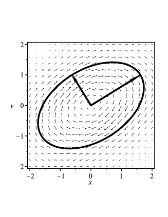
Figure 1: An elliptical contour line of the distribution of a trapped particle in a linear shear flow is shown, cf. Eq. (8) with $\alpha=0,\beta=1$, as well as the vector field $\mathbf{j}(x,y)$. The broad arrows indicate the two principal axes of the ellipse.

The parameter $\alpha$, describing the contribution of the uniform flow, causes essentially a shift of the distribution $\mathcal{P}_{ab}(x,y)$ in the $x$-direction. In the following we consider the case $\alpha=0$, where $a_{4}=a_{5}=0$ and the resulting distribution function is denoted by $\mathcal{P}_{a}(x,y)$. Its elliptical contour lines can be characterized by two principal axes. The ratio between their lengths as well as the angle between the major principal axis and the flow direction are a function of the Weissenberg number $\beta$. This was already discussed in Ref. Holzer:2009.1 , where shear-induced corrections to the autocorrelations as well as a cross-correlation between orthogonal particle fluctuations in the shear plane were found. These correlations can also be calculated in terms of the probability distribution $\mathcal{P}_{a}(x,y)$ via the expression $\langle r_{i}r_{j}\rangle=\int\int dxdy\mathcal{P}_{a}(x,y)r_{i}r_{j}$:

$$\langle xx\rangle=1+\frac{\beta^{2}}{2},\quad\langle xy\rangle=\langle yx\rangle=\frac{\beta}{2},\quad\langle yy\rangle=1\,.$$ (10)

After rescaling to dimensional units, $x\to\bar{x}$, the results given in Ref. Holzer:2009.1 are recovered.

In a plane Poiseuille flow all three parameters $\alpha$, $\beta$ and $\gamma$ in the SE (6) may be non-zero and no exact analytical solution was found in this case. Similar to vdVen:1980.1 , the probability distribution is calculated perturbatively and compared with numerical solutions of Eq. (6).

First we consider a Brownian particle which is trapped at the center of a plane Poiseuille flow, with $\tilde{y}_{0}=0$. In this case of vanishing $\beta$, the parameter $\alpha=u_{p}\delta\zeta/(k_{B}T)$ describes the ratio between the drag force imposed by the flow and the potential force on the particle. If $\alpha$ is fixed, the parameter $\gamma=-\alpha(\delta/l)^{2}$ depends on the ratio between the two characteristic lengths $l$ and $\delta$. Note, the hydrodynamic interactions between the particle and the walls are small in the range $\delta/l<1/2$.

Our ansatz for the perturbation expansion of the solution of Eq. (6) up to the second order in $\gamma$ reads

$$\mathcal{P}(x,y)=\mathcal{P}_{n}(x,y)~{}e^{\gamma f_{1}(x,y)+\gamma^{2}g_{1}(x,y)}\,,$$ (11)

with the two polynomials

$$f_{1}(x,y) =b_{1}x+b_{2}y^{2}+b_{3}xy^{2}\,,$$ (12a)

$$g_{1}(x,y) =(c_{1}x+c_{2}x^{2})(1+y^{2})+c_{3}y^{2}+c_{4}y^{4}\,.$$ (12b)

The SE (6) may then be rewritten:

$$\left(p_{0}(x,y)+\gamma p_{1}(x,y)+\gamma^{2}p_{2}(x,y)\right)\mathcal{P}(x,y)=0\,.$$ (13)

Since $\gamma$ is an arbitrary, but small number, the polynomials $p_{0,1,2}(x,y)$ in Eq. (13) have to vanish separately. According to Eq. (8) the condition $p_{0}(x,y)=0$ is automatically fulfilled. The second condition, $p_{1}(x,y)=0$, provides the first-order coefficients

$$b_{1}=\frac{2}{3},\quad b_{2}=\frac{-\alpha}{3},\quad b_{3}=\frac{1}{3}\,,$$ (14)

whereas the third condition, $p_{2}(x,y)=0$, determines the coefficients at $\mathcal{O}(\gamma^{2})$:

$$c_{1}=\frac{-2\alpha}{9},\quad c_{2}=\frac{1}{9},\quad c_{3}=\frac{\alpha^{2}}{9}-\frac{1}{3},\quad c_{4}=\frac{-1}{18}\,.$$ (15)

With the potential minimum off the center of the Poiseuille flow, one has $\tilde{y}_{0}\neq 0$, a finite Weissenberg number $\beta\neq 0$ and no longer $\pm y$ symmetry. Again we use an ansatz of the form:

$$\mathcal{P}(x,y) =\mathcal{P}_{ab}(x,y)\,e^{\gamma f_{2}(x,y)+\gamma^{2}g_{2}(x,y)}\,.$$ (16)

Due to the loss of the $\pm y$ symmetry, the polynomial $f_{2}(x,y)$ has nine different contributions:

$$f_{2}(x,y)= d_{1}x+d_{2}y+d_{3}(x-3\alpha)x^{2}+d_{4}(x-\alpha)y^{2}$$

$$+d_{5}(x-2\alpha)xy+d_{6}y^{3}\,.$$ (17)

The condition that the $\mathcal{O}(\gamma)$-terms in Eq. (6) have to vanish determines the coefficients in the ansatz (The probability distribution of a trapped Brownian particle in plane shear flows). With $B=\beta^{2}+4$ and $E=2/(9B^{3})$ they are given by

$$d_{1} =4E\left((12-\beta^{2})B+16\alpha^{2}\beta^{2}\right),$$

$$d_{2} =-2E\beta\left((20+\beta^{2})B+8\alpha^{2}(\beta^{2}-4)\right),$$

$$d_{3} =\frac{64}{3}E\beta^{2}\,,~{}~{}~{}d_{4}=2E(3\beta^{4}-8\beta^{2}+48),$$

$$d_{5} =16E\beta(4-\beta^{2}),$$

$$d_{6} =\frac{-E\beta}{3}(5\beta^{4}+24\beta^{2}+144)\,.$$ (18)

In the limit $\beta\to 0$ the coefficients (14) are recovered. The polynomial $g_{2}(x,y)$ for the order $\gamma^{2}$ includes $14$ lengthy contributions, which we do not list here.

In order to estimate the validity range of the approximations presented above, we determine stationary solutions of the SE. (6) numerically. To this end a simple Jacobi-relaxation method, cf. Ref. NumResF , or a direct integration of the rescaled Eq. (3) is sufficient. The probability current is determined via:

$$\mathbf{j} =-\nabla\mathcal{P}+\left[\begin{pmatrix}\alpha+\beta y+\gamma y^{2}\\ 0\end{pmatrix}-\begin{pmatrix}x\\ y\end{pmatrix}\right]\mathcal{P}\,.$$ (19)

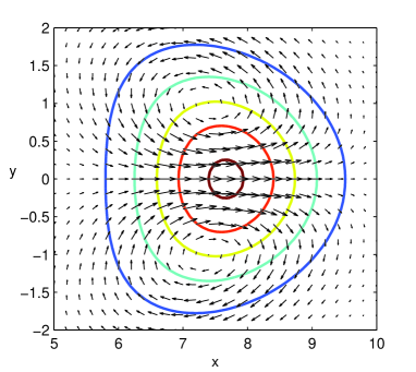
Figure 2: Contour lines of the numerical solution of Eq. (6) as well as the vector field $\mathbf{j}(x,y)$ are shown for the case where the potential minimum is at the center of a plane Poiseuille flow. Parameters: $\alpha=8,~{}\gamma=-\alpha(\delta/l)^{2}=-1/2$.

Fig. 2 shows the contour lines of the numerically obtained probability distribution $\mathcal{P}(x,y)$ in the case with the minimum of the trapping potential at the center of a plane Poiseuille flow. This distribution has similarities with the parachute or bullet-like shape of vesicles in a Poiseuille flow Skalak:1969.1 ; Gompper:2005.1 ; Misbah:2009.1 . In comparison to similar numerical results, obtained via the related Langevin equation and presented in Ref. Holzer:2009.1 , we additionally show the probability current $\mathbf{j}(x,y)$. As indicated in Fig. 2, the vector field $\mathbf{j}({x,y})$ includes two counter-rotating vortices that are symmetric with respect to the $x$-axis.

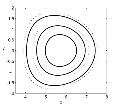
Figure 3: Comparison of the numerically determined distribution (solid lines) with the analytical approximations, given by Eq. (11) (dashed lines). The contour lines of both types are plotted at different heights in order to distinguish them to compare their shapes. Parameters: $\alpha=6$, $\gamma=-3/8$.

In Fig. 3 contour lines of the numerically obtained probability distribution are compared with those obtained from the perturbative solution (11) for the parameters $\alpha=6$ and $\gamma=-\alpha(\delta/l)^{2}=-3/8$. In spite of this rather large $|\gamma|$-value, beyond the expected validity range of the perturbation expansion, the differences between both solutions in Fig. 3 are surprisingly small. As expected, for decreasing values of $|\gamma|$ these differences become even smaller, but the analytical formula (11) may be useful for fitting experimental data up to $|\gamma|\simeq 3/8$.

The symmetrical shape of the distribution is lost if the particle is trapped away from the center of the plane Poiseuille flow. With increasing values of $\tilde{y}_{0}$ and $\beta$, the shape of the probability distribution deforms from a parachute or bullet towards an ellipse. Simultaneously one vortex of the probability current is enhanced while the other one is weakened. For the values $\tilde{y}_{0}=l/4$, $\delta/l=1/4$ and $\alpha=7$, with $\beta=-2\alpha/15$ and $\gamma=-\alpha/15$, the contour lines of $\mathcal{P}(x,y)$ as well as the current $\mathbf{j}(x,y)$ are displayed in Fig. 4. In this case the lower vortex in $\mathbf{j}(x,y)$ has already vanished and the distribution $\mathcal{P}(x,y)$ shares similarities with the slipper shape of vesicles in capillary flows Misbah:2009.2 . Again the results are in good agreement with the simulations in Ref. Holzer:2009.1 .

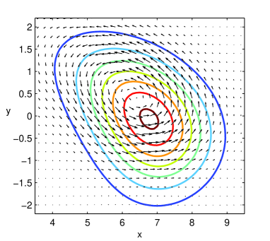
Figure 4: Contour lines of $\mathcal{P}(x,y)$ and vector field $\mathbf{j}(x,y)$ for the case where the potential minimum is off the center of the Poiseuille flow. Parameters: $\alpha=7,\beta=-14/15,\gamma=-7/15$.

In conclusion, we investigated the positional distribution of a Brownian particle, which is trapped by a harmonic potential and simultaneously exposed to different shear flows. A complete analytical solution of the corresponding Smoluchowski equation is given in the case of a linear shear flow. For a plane Poiseuille flow, we presented approximate analytical formulas, which are in good agreement with numerical solutions for a wide range of parameters. Some of our results confirm earlier ones obtained in Ref. Holzer:2009.1 on the basis of simulations of the related Langevin equation.

Our predictions of the particle’s probability distribution in a Poiseuille flow may be measured in an experiment similar to that in Ref. Ziehl:2009.1 . In this work, a micron-sized polystyrene bead was trapped by an optical tweezer and the fluctuating particle positions were recorded by a high speed camera in a stroboscopic manner. For the positions of a trapped particle in Poiseuille flow one expects probability distributions as predicted in this work. The presented analytical approximations for the particle distribution may be useful for fitting the experimental data.

Experiments with particles placed near the center of a Poiseuille flow, where the flow velocity takes its maximum value, may require large laser intensities in order to keep the particles trapped by the potential. This constraint reduces the flexibility for variations of the typical length scale $\delta$ of the particle’s positional fluctuations. Since the flow profile determines the shape of the particle distribution and not the flow velocity near the potential minimum, one may reduce the drag force by moving the trap along with the flow.

The statistical properties of trapped Brownian particles, as investigated in Quake:2000.1 ; Ziehl:2009.1 ; Holzer:2009.1 , share similarities with those of tethered polymers exposed to uniform flows Chu:1995.1 ; Brochard:1993.1 ; Rzehak:99.2 ; Rzehak:2000.1 or to shear flows Doyle:2000.1 . The related theoretical explorations are mainly based on Brownian dynamics simulations. An interesting question is, how far can the analysis described here be applied to tethered bead-spring models in shear flows? Do such investigations exhibit temporal oscillations as found for instance for deterministic models Holzer:2006.1 ?

We thank M. Burgis for inspiring discussions. This work was supported by DFG via the priority program on micro- and nanofluidics SPP 1164, and by the Bayerisch-Französisches Hochschulzentrum.

References

- (1) J. K. G. Dhont, An Introduction to Dynamics of Colloids (Elsevier, Amsterdam, 1996).
- (2) H. Berg, Random Motions in Biology (Princeton Univ. Press, Princeton, 1993).
- (3) R. T. Foister and T. G. M. van de Ven, J. Fluid Mech. 96, 105 (1980).
- (4) Y. Drossinos and M. W. Reeks, Phys. Rev. E 71, 031113 (2005).
- (5) D. C. Swailes, Y. Ammar, M. W. Reeks, and Y. Drossinos, Phys. Rev. E 79, 036305 (2009).
- (6) M. H. Vainstein and J. M. Rubi, Phys. Rev. E 75, 031106 (2007).
- (7) K. Miyazaki and D. Bedeaux, Physica 217A, 53 (1995).
- (8) G. Subramanian and J. Brady, Physica 334A, 343 (2004).
- (9) A. Ziehl, J. Bammert, L. Holzer, C. Wagner, and W. Zimmermann, Phys. Rev. Lett. 103, 230602 (2009).
- (10) L. Holzer, J. Bammert, R. Rzehak, and W. Zimmermann, Phys. Rev. E 81, 041124 (2010).
- (11) J. Bammert, L. Holzer, and W. Zimmermann, arXiv:1006.1560 (2010).
- (12) H. Risken, The Fokker-Planck Equation: Methods of Solution and Applications (Springer-Verlag, Berlin, 1989).
- (13) W. H. Press, S. A. Teukolsky, W. T. Vetterling, and B. P. Flannery, Numerical Recipes in Fortran: The Art of Scientific Computing, 2nd ed. (Cambridge University Press, Cambridge, England, 1992).
- (14) R. Skalak and P. I. Branemar, Science 164, 717 (1969).
- (15) H. Noguchi and G. Gompper, Proc. Nat. Acad. Sci. 102, 14159 (2005).
- (16) G. Danker, P. M. Vlahovska, and C. Misbah, Phys. Rev. Lett. 102, 148102 (2009).
- (17) B. Kaoui, G. Biros, and C. Misbah, Phys. Rev. Lett. 103, 188101 (2009).
- (18) J. C. Meiners and S. R. Quake, Phys. Rev. Lett. 84, 5014 (2000).
- (19) T. Perkins, D. Smith, R. Larson, and S. Chu, Science 268, 83 (1995).
- (20) F. Brochard-Wyart, Europhys. Lett. 23, 105 (1993).
- (21) R. Rzehak, D. Kienle, T. Kawakatsu, and W. Zimmermann, Europhys. Lett. 46, 821 (1999).
- (22) R. Rzehak, W. Kromen, T. Kawakatsu, and W. Zimmermann, Eur. Phys. J. E 2, 3 (2000).
- (23) P. S. Doyle, B. Ladoux, and J. L. Viovy, Phys. Rev. Lett. 84, 4769 (2000).
- (24) L. Holzer and W. Zimmermann, Phys. Rev. E 73, 060801(R) (2006).