Models of self-financing hedging strategies in illiquid markets:
symmetry reductions and exact solutions
Ljudmila A. Bordag, Anna Mikaelyan
IDE, MPE Lab,
Halmstad University, Box 823,
301 18 Halmstad, Sweden

Abstract
We study the general model of self-financing trading strategies in illiquid markets introduced by Schönbucher and Wilmott, 2000. A hedging strategy in the framework of this model satisfies a nonlinear partial differential equation (PDE) which contains some function $g(\alpha)$. This function is deep connected to an utility function.

We describe the Lie symmetry algebra of this PDE and provide a complete set of reductions of the PDE to ordinary differential equations (ODEs). In addition we are able to describe all types of functions $g(\alpha)$ for which the PDE admits an extended Lie group. Two of three special type functions lead to models introduced before by different authors, one is new. We clarify the connection between these three special models and the general model for trading strategies in illiquid markets. We study with the Lie group analysis the new special case of the PDE describing the self-financing strategies. In both, the general model and the new special model, we provide the optimal systems of subalgebras and study the complete set of reductions of the PDEs to different ODEs. In all cases we are able to provide explicit solutions to the new special model. In one of the cases the solutions describe power derivative products.

Keywords: nonlinear PDEs; illiquid markets; option pricing; invariant reductions; exact solutions;

MSC code: 35K55, 34A05, 22E60

Corresponding author: Ljudmila A. Bordag, Ljudmila.Bordag@hh.se

1 Introduction

We study self-financing hedging strategies in the framework of a reaction-function model. The main subject of this model is a smooth reaction function $\psi$ that gives the equilibrium stock price $S_{t}$ at time $t$ as function of some fundamental value $F_{t}$ and the stock position of a large trader. In the framework of this model there are two types of traders in the market: ordinary investors and a large investor. The overall supply of the stock is normalized to one. The normalized stock demand of the ordinary investors at time $t$ is modeled as a function $D(F_{t},S_{t})$, where $S_{t}$ is the proposed price of the stock. The normalized stock demand of the large investor is written in the form $\rho\Phi_{t}$; $\rho\geq 0$ is a parameter that measures the size of the trader’s position relative to the total supply of the stock. The equilibrium price $S_{t}$ is then determined by the market clearing condition

$$D(F_{t},S_{t})+\rho\Phi_{t}=1\,.$$ (1.1)

The equation (1.1) admits a unique solution $S_{t}$ under suitable assumptions on the function $D(F_{t},S_{t})$. Hence $S_{t}$ can be expressed as a function $\psi$ of $F_{t}$ and $\rho\Phi_{t}$, so that $S_{t}=\psi(F_{t},\rho\Phi_{t})$.

Now we turn to the characterization of self-financing hedging strategies in the framework of the reaction-function model. Throughout we assume that the fundamental value process $F_{t}$ follows a geometric Brownian motion with volatility $\sigma$ as in the Black-Scholes model. Moreover, we assume that the reaction function $\psi(F_{t},\rho\Phi_{t})$ is of the form

$$\psi(f,\alpha)=f~{}g(\alpha)$$ (1.2)

with some increasing function $g(\alpha)$. This holds for any model where

$$D(f,s)=U(f/s)$$ (1.3)

for a strictly increasing function $U:(0,\infty)\to\mathbb{R}$ with a suitable range.

Assuming as before that the normalized trading strategy of the large trader is of the form $\rho\Phi(t,S)$ for a smooth function $\Phi$, we get from Itô’s formula that

$$dS_{t}=g(\rho\Phi(t,S_{t}))\,dF_{t}+\rho F_{t}g_{\alpha}(\rho\Phi(t,S_{t}))\Phi_{S}(t,S_{t})\,dS_{t}+b(t,S_{t})\,dt$$ (1.4)

(since $S_{t}=g(\rho\Phi(t,S_{t}))F_{t}$). The precise form of $b(t,S_{t})$ is irrelevant to our purposes. Assume now that

$$\big{(}1-\rho F_{t}g_{\alpha}(\rho\Phi(t,S_{t}))\Phi_{S}(t,S_{t})\big{)}>0\quad\rm{a.s.}.$$ (1.5)

This can be viewed as an upper bound on the permissible variations of the large trader’s strategy. Rearrangement and integration $\big{(}1-\rho F_{t}g_{\alpha}(\rho\Phi(t,S_{t}))\Phi_{S}(t,S_{t})\big{)}^{-1}$ over both sides of equation (1.4) gives us the following dynamics of $S$:

$$dS_{t}=\frac{1}{1-\rho\frac{g_{\alpha}(\rho\phi(t,S_{t}))}{g(\rho\phi(t,S_{t}))}S_{t}\phi_{S}(t,S_{t})}\sigma S_{t}dW_{t}+\tilde{b}(t,S_{t})dt\,,$$ (1.6)

again the precise form of $\tilde{b}$ is irrelevant.

If we apply the Ito-Wentzell formula [1] to this equation we obtain the following PDE for a self-financing hedging strategy

$$u_{t}+\frac{1}{2}\frac{\sigma^{2}S^{2}u_{SS}}{\left(1-\rho\frac{g^{\prime}(\rho u_{S})}{g(\rho u_{S})}Su_{SS}\right)^{2}}=0.$$ (1.7)

Under some special choices of the function $g(\alpha)$ equation (1.7) represents the models introduced earlier.
If we take $g(\alpha)=c_{2}e^{c_{1}\alpha}$, $c_{1},c_{2}-const.$ we obtain the model introduced in [10]. This model was studied with Lie group methods in [7], [8] and some generalization of this model in [6].
In the case of $g(\alpha)=c_{2}(\rho+k\alpha)^{-\frac{1}{c_{1}}}$, $c_{1},c_{2},k-const.$ equation (1.7) coincides with the models introduced in [15] and studied with Lie group methods in [4] and [5].

The main goal of this paper is to study the analytical properties of equation (1.7) in the first line with the Lie group method. We will clarify which symmetry properties has this equation and under which additional conditions on the function $g(\alpha)$ it admits a richer symmetry group.

If the symmetry group admitted by an equation is known then it can be used in many cases to reduce the given equation to a simpler one, for instance, to an ODE or even solve it. Solutions of such reduced equations are called invariant solutions because they are invariant under the action of the corresponding subgroup of the symmetry group of this equation. We follow this strategy and describe the complete set of reductions for the general model (1.7) in section 3.

In addition we obtain also some special forms of utility functions for which the corresponding equation admits a richer symmetry group. The connection between the function $g(\alpha)$ and the utility function is described in section 2. For a special form of utility function we obtain a special model for hedging strategies in illiquid markets. This special model is studied in section 4. Also for this model we present an optimal system of subalgebras, the complete set of reductions to ODEs. In this case we are able to solve all the ODEs and provide explicit formulas or graphs of solutions.

2 The function $g(\alpha)$, the corresponding utility function and the self-financing hedging strategy

We use the classical assumptions (see [9]) on a utility function $U(x)$, modeling the utility of a market participant’s wealth $x$ at fixed time.

Definition 2.1

Let $U(x)$ is a utility function. Then $U:\mathbb{R}\to\mathbb{R}\cup\{-\infty\}$

1. is increasing on $\mathbb{R}$, continuous on $\{U>-\infty\}$, differentiable and strictly concave on the interior of $\{U>-\infty\},$

2. $U^{\prime}(\infty)=\lim_{x\to\infty}U^{\prime}(x)=0,$

3. if a negative wealth is not allowed then $U(x)=-\infty,$ for $x<0$, $U(x)>-\infty,$ for $x>0$, and the Inada condition $U^{\prime}(0)=\lim_{x\to 0,x>0}U^{\prime}(x)=\infty$ holds,

4. if a negative wealth is allowed then $U(x)>-\infty,$ for $x\in\mathbb{R}$ and $U^{\prime}(-\infty)=\lim_{x\to-\infty}U^{\prime}(x)=\infty$ holds.

Using the form of the factor representation of the reaction function (1.2) and (1.3) we obtain the following equation for the utility function

$$U\left(\frac{1}{g(\alpha)}\right)=1-\alpha.$$ (2.8)

We restrict our consideration further to the case where a negative wealth is not allowed and consider the utility function $U$ as a map $U:\mathbb{R}^{+}\to\mathbb{R}\cup\{-\infty\}$ with the assumptions (1) – (3) listed in the Definition 2.1 above.

Because of this we can restrict the argument of the utility function $U(x)$ on $\mathbb{R}^{+}$, hence we look for a function $g(\alpha)>0$. We are able to rewrite the relation (2.8) in a more convenient and explicit form for some typical special forms of the function $g(\alpha)$:

1. If the function $g(\alpha)$ takes the form $g(\alpha)=c_{2}e^{c_{1}\alpha}$ then it corresponds to the utility function which is equal to

   $$g(\alpha)=c_{2}e^{c_{1}\alpha},~{}~{}\to~{}~{}U(x)=\frac{1}{c_{1}}\ln x+\frac{c_{1}+\ln c_{2}}{c_{1}},~{}c_{1},c_{2}\neq 0.$$ (2.9)

   Because the argument of the utility function should be positive the function $g(\alpha)=c_{2}e^{c_{1}\alpha}$ should be positive too, i.e. the coefficient $c_{2}$ should be strictly positive $c_{2}>0$. According to the assumption (1) of Definition 2.1 the utility function $U(x)$ should be an increasing function, then $c_{1}>0$. It is easy to prove that all other assumptions are as well satisfied for the utility function of the form (2.9) by $c_{1},c_{2}>0$.
   The PDE for the self-financing hedging strategy takes in this case the following form

   $$u_{t}+\frac{1}{2}\frac{\sigma^{2}S^{2}u_{SS}}{\left(1-\rho c_{1}Su_{SS}\right)^{2}}=0.$$ (2.10)

   This equation was first introduced in [10]. The complete description of the symmetry group, invariant reductions and invariant solutions to this equation as well as to some generalization of this equation are given in [6], [7] and [8].

2. If the function is given by $g(\alpha)=c_{2}\alpha^{c_{1}}$ then the corresponding utility function takes the form

   $$g(\alpha)=c_{2}\alpha^{c_{1}},~{}~{}\to~{}~{}U(x)=-(c_{2}x)^{-\frac{1}{c_{1}}}+1.$$ (2.11)

   Under our assumption the utility function acts on $(0,+\infty)$ correspondingly the function $g(\alpha)=c_{2}\alpha^{c_{1}}$ should be positive. The assumptions (1) – (3) of Definition 2.1 are satisfied if

   $$c_{1},c_{2}>0.$$ (2.12)

   The PDE which corresponds to this function $g(\alpha)$ has the form

   $$u_{t}+\frac{1}{2}\frac{\sigma^{2}S^{2}u_{SS}u_{S}^{2}}{(u_{S}-c_{1}Su_{SS})^{2}}=0.$$ (2.13)

   This equation is the special model for hedging strategies in illiquid markets which we will study in the section 4 of this paper.

3. If we take similar to the previous case the function $g(\alpha)$ in the form $g(\alpha)=c_{2}(\rho+k\alpha)^{-\frac{1}{c_{1}}}$, where $c_{1},c_{2},k\in{\mathbb{R}},~{}~{}k\neq 0$ then the corresponding utility function is given by

   $$g(\alpha)=c_{2}(\rho+k\alpha)^{-\frac{1}{c_{1}}},~{}~{}\to~{}~{}U(x)=-\frac{1}{k}(c_{2}x)^{c_{1}}+\left(1+\frac{\rho}{k}\right).$$ (2.14)

   The utility function acts on $(0,+\infty)$ because of that the function $g(\alpha)=c_{2}(\rho+k\alpha)^{-1/c_{1}}$ should be positive.

   The assumptions of Definition 2.1 on the the utility function acting on $(0,+\infty)$ are satisfied if

   $$c_{2}>0,~{}~{}c_{1}\in(-\infty,0)\cup(0,1),~{}~{}kc_{1}>0.$$ (2.15)

   The PDE for a self-financing trading strategy takes in this case the form

   $$u_{t}+\frac{1}{2}\frac{\sigma^{2}(1+ku_{S})^{2}}{c_{1}^{2}\left(1+ku_{S}+\frac{k}{c_{1}}Su_{SS}\right)^{2}}S^{2}u_{SS}=0\,,{c_{1}}\neq 0,$$ (2.16)

   This equation coincides with some of the models introduced in [15]). This model was studied with the Lie group method in [4] and [5]. The corresponding symmetry algebra admitted by this equation, an optimal system of subalgebras, the set of invariant reductions and in some cases also exact invariant solutions are presented in these papers.

3 The Lie algebra admitted by the general model (1.7)

To study the symmetry properties of (1.7) we use the method introduced by Sophus Lie and developed further in [17], [16] and [11]. For the first reading also the books [19] and [2] can be used which contain many examples.

The main idea of this method can be formulated in the following way. We introduce first a jet-bundle of the corresponding order (in this case of the order two, because of we have to do with a second order PDE). Then we study all smooth point transformations which locally keep the solution subvariety of the studied PDE invariant. Sophus Lie has proved that instead to look for the symmetry group we can first study the symmetry algebra of the underlying PDE and then with help of an exponential map we obtain the corresponding symmetry group. We follow these ideas and determine the symmetry algebra admitted by the equation.

Let us introduce now the necessary notations.
We have two sets of variables, the independent variables ${t,S}$ which are in the space $X$, $(t,S)\in X$ and a dependent variable ${u}$ which belongs to the space $U$, i.e. $u\in U$.
We consider the second prolongation of the space $U$. We first introduce the space $U_{(1)}$. It is the Euclidean space endowed with coordinates $(u_{t},u_{S})$ which represent all first derivatives of $u$ with respect to $(t,S)$. Then we introduce the space $U_{(2)}$, it is the space endowed with coordinates $(u_{tt},u_{tS},u_{SS})$ which represent all second derivatives of $u$ with respect to $(t,S)$. Now we can define the second prolongation of $U$ and a jet bundle of the order two.

Definition 3.1

The $2-$nd prolongation of $U$ is $U^{(2)}=U\times U_{(1)}\times U_{(2)}$ .

Definition 3.2

The $2-$nd jet bundle of $M\subset X\times U$, or the jet bundle of order two, is $M^{(2)}=M\times U_{(1)}\times U_{(2)}=X\times U^{(2)}$. $M^{(2)}$ also called $2-$nd prolongation of $M$, it is also denoted by $pr^{(2)}M$.

We write the PDE (1.7) in the form

$$\Delta(w)=\Delta(x,u^{(2)})=\Delta(t,S,u,u_{t},u_{S},\dots,u_{SS})=0,~{}~{}w\in M^{(2)},~{}~{}u^{(2)}\in U^{(2)}.$$ (3.17)

Here $\Delta$ is a smooth map from the jet bundle $M^{(2)}$ to some Euclidean space $\mathbb{R}$, i.e. $\Delta:M^{(2)}\to{\mathbb{R}}$. It defines the solution subvariety

$${L}_{\Delta}=\{(x,u^{(2)}):\Delta(x,u^{(2)})=0\}\subset M^{(2)}.$$

The symmetry group $G_{r}$ of $\Delta$ will be defined by

$$G_{r}=\{g\in{\rm{Diff}(M^{(2)})}{|}~{}~{}g:~{}~{}L_{\Delta}\to L_{\Delta}\},~{}~{}r=\dim G_{r}.$$ (3.18)

The symmetry algebra $L_{r}={\mathcal{D}iff}_{\Delta}(M)$ of the PDE $\Delta(w)=0$ can be found as a solution of the determining equations

$$pr^{(2)}V(\Delta)=0~{}(mod(\Delta(w)=0)),$$ (3.19)

where $pr^{(2)}V$ denotes the second prolongation of an infinitesimal generator $V$ and has the following form

$$pr^{(2)}V = \xi(S,t,u)\frac{\partial}{\partial S}+\tau(S,t,u)\frac{\partial}{\partial t}+\varphi(S,t,u)\frac{\partial}{\partial u}$$

$$+ \varphi^{S}(S,t,u)\frac{\partial}{\partial u_{S}}+\varphi^{t}(S,t,u)\frac{\partial}{\partial u_{t}}$$

$$+ \varphi^{SS}(S,t,u)\frac{\partial}{\partial u_{SS}}+\varphi^{St}(S,t,u)\frac{\partial}{\partial u_{St}}+\varphi^{tt}(S,t,u)\frac{\partial}{\partial u_{tt}}.$$

Here the last five coefficients can be uniquely defined using the first three (see [16]). The determining equations (3.19) is a system of PDEs on the functions $\xi(S,t,u)$, $\tau(S,t,u)$ and $\varphi(S,t,u)$. The solution of this system provides us all infinitesimal generators admitted by the studied equation. The set of these infinitesimal generators forms a Lie algebra which is called the Lie algebra admitted by the PDE $\Delta(w)=0$ or the symmetry algebra of this equation. The determining equations and the corresponding solutions to equation (1.7) are presented in detail in [13].

We formulate the main result concerning the equation (1.7) where we do not put any constrains on the form of the function $g(\alpha)$. We just assume that this function is a differentiable one. In this case we obtain the following theorem.

Theorem 3.1

The equation (1.7), where $g(\alpha)$ is a differentiable function, admits a three dimensional Lie algebra $L_{3}$ spanned by the following generators

$$L_{3}=<V_{1},V_{2},V_{3}>,~{}~{}V_{1}=S\frac{\partial}{\partial S}+u\frac{\partial}{\partial u},~{}~{}V_{2}=\frac{\partial}{\partial u},~{}~{}V_{3}=\frac{\partial}{\partial t}.$$ (3.21)

The Lie algebra $L_{3}$ possesses a nonzero commutator relation $[V_{1},V_{2}]=-V_{2}.$ The Lie algebra $L_{3}$ has a two-dimensional subalgebra $L_{2}=<V_{1},V_{2}>$ spanned by the generators $V_{1},V_{2}$. The algebra $L_{3}$ is a decomposable Lie algebra and can be represented as a semi-direct sum $L_{3}=L_{2}\bigoplus V_{3}$.

The determining equations (3.19) admit a richer set of solutions if the function $g(\alpha)$ has a special form. We proved (see for details [13]) that equation (1.7) admits a four dimensional Lie algebra if and only if the function $g(\alpha)$ has one of the following forms:

$$g(\alpha) = c_{2}e^{c_{1}\alpha},$$ (3.22)

$$g(\alpha) = c_{2}\alpha^{c_{1}},$$ (3.23)

$$g(\alpha) = c_{2}(\rho+k\alpha)^{-\frac{1}{c_{1}}},~{}~{}c_{1},c_{2},k-{\rm const.}.$$ (3.24)

We discussed in the previous section relations between the given form of the function $g(\alpha)$ and the corresponding utility function. We provided also the PDEs related to the special choice of the function $g(\alpha)$. As we mentioned before the first and the last case, i.e. the equations (2.10) and (2.16) were studied with the Lie group analysis before. The second case, i.e. equation (2.13) will be studied in section 4.

The Lie algebra $L_{3}$ is the symmetry algebra of equation (1.7). Using the usual exponential map we can find the symmetry group $G_{3}$ of this equation as well. It is not necessary to find the explicit form of the symmetry group $G_{3}$ if we will use invariants of this group or its subgroups to find reductions and invariant solutions of the studied equation. It is enough to know and to use the properties of the symmetry algebra which corresponds to the symmetry group. The most interesting reductions we obtain if we use one-dimensional subalgebras of $L_{3}$ (and corresponding subgroups of $G_{3}$). The problem how to choose the optimal system of subalgebras (and correspondingly subgroups) which give us non-conjugate invariant solutions was solved 1982 by Ovsiannikov (see [17]). We follow the algorithm of determining of an optimal system of subalgebras proposed there.

We use the notation $h_{i}^{g}$ for the subalgebras of the Lie algebra $L_{3}$ and $H_{i}^{g}$ for the corresponding subgroups of the group $G_{3}$. All three- and four-dimensional solvable algebras were classified in [18]. In addition in this paper there are provided optimal systems of corresponding subalgebras. We use these results in this and in the next section.

Proposition 3.1

[18].   The optimal system of subalgebras of $L_{3}$ contains the subalgebras shown in Table 2

Dimension of	Subalgebras
the subalgebra
1	$h_{1}^{g}=\left\{V_{2}\right\},~{}h_{2}^{g}=\left\{V_{1}\cos(\varphi)+V_{3}\sin(\varphi)\right\},~{}h_{3}^{g}=\left\{V_{2}+\epsilon~{}V_{3}\right\}$
2	$h_{4}^{g}=\big{(}V_{2},V_{3}\big{)},~{}h_{5}^{g}=\big{(}V_{1},V_{3}\big{)},~{}h_{6}^{g}=\big{(}V_{1}+x~{}V_{3},V_{2}\big{)}$

Table 1: The optimal system of one- and two-dimensional subalgebras of $L_{3}$, where parameters are $x\in\mathbb{R},~{}0\leq\phi\leq\pi,~{}\epsilon=\pm 1$.

3.1 The symmetry reductions of the general model (1.7)

There are three non-similar subalgebras of the dimension one which we list in Table 2. To each of these subalgebras corresponds a one-dimensional subgroup and they form the set of non-conjugate subgroups. We use the optimal system of subalgebras for invariant reductions of the equation (1.7) to ODEs. To obtain reduced form of the PDE we take invariant expressions as a new dependent and an independent variables and in the new variables we obtain ODEs.

Subalgebra	Invariants	Transformations/Reductions
$h_{1}^{g}$	$z=S,~{}W(z)=t$	$u\rightarrow u+\rm{const}.$
$h_{2}^{g}$	$z=S,~{}W(z)=u-\epsilon t$	$2\epsilon+\frac{\sigma^{2}z^{2}Y^{\prime}}{\left(1-z(\ln g(\rho Y))^{\prime}\right)^{2}}=0,~{}Y=W^{\prime},$
		$g(\rho Y(z))\neq cz.$
$h_{3}^{g}$	$z=\ln S-\gamma~{}t~{}$,$~{}\gamma={\rm cotan}(\phi)~{}$	$2\gamma Y-\frac{\sigma^{2}(Y^{\prime}+Y)}{(1-(\ln g(Y^{\prime}+Y))^{\prime})^{2}}=0,$
	$W(z)=uS^{-1}$
		$~{}Y=W^{\prime},~{}~{}g(Y+Y^{\prime})\neq ce^{z}$.

Table 2: In the first row we list one-dimensional subalgebras from the optimal system of $L_{3}$ (3.21). In the second row we list the corresponding invariants. In the last row we provide the transformations or reductions of the PDE (1.7) to ODEs. Here $\epsilon=\pm 1,~{}0\leq\phi\leq\pi,~{}\sigma^{2},\rho\in\mathbb{R^{+}},c\in\mathbb{R}$ are parameters, $Y^{\prime},W^{\prime}$ denote the differentiation of the corresponding function on the invariant variable $z$.

In the first line of Table 2 we see that the first subgroup $H_{1}^{g}$ describes translations of the dependent variable $u$ and can not be used for any reduction.

In the case of the subgroup $H_{2}^{g}$ the reduction of the given PDE to an ODE is possible. But the solutions to the general model (1.7) of this type are not very interesting because of they have a trivial dependence on time (see the second row, second line in Table 2). The most interesting case we obtain if we use the subgroup $H_{3}^{g}$. We obtain solutions to (1.7) of the form $u(S,t)=SW(\ln S-\gamma t)$ if we are able to solve the first order ODE which is represented in the last row and last line of Table 2. It is rather impossible to present a general solution to this equation for an arbitrary function $g(\alpha)$, but for some special choices of $g(\alpha)$ it seems to be feasible.

4 Symmetry properties of the special model (2.13)

We mentioned before that for some special types of the function $g(\alpha)$ (3.22)-(3.24) the equation (1.7) admits four dimensional Lie algebras. Because two of these cases (3.22)-(3.24) were studied before we investigate now the last one, i.e. the symmetry properties of the special model (2.13) with the function $g(\alpha)$ in the form (3.23).

This equation (2.13) contains an arbitrary constant $c_{1}$ but it does not include any more the parameter $\rho$. The solution of the determining equation (3.19) defines four generators of the Lie algebra $L_{4}$. We formulate the results in the following Theorem.

Theorem 4.1

Equation (2.13) admits a four dimensional Lie algebra

$$L_{4}=<V_{1},V_{2},V_{3},V_{4}>$$

spanned by generators

$$V_{1}=S\frac{\partial}{\partial S},~{}~{}V_{2}=u\frac{\partial}{\partial u},~{}~{}V_{3}=\frac{\partial}{\partial u},~{}~{}V_{4}=\frac{\partial}{\partial t}.$$ (4.25)

The Lie algebra $L_{4}$ possesses the following non-zero commutator relation, $[V_{1},V_{3}]=-V_{3}.$ The Lie algebra $L_{4}$ has a two-dimensional subalgebra $L_{2}^{4}=<V_{1},V_{3}>$ spanned by the generators $V_{1},V_{3}$. The algebra $L_{4}$ is a decomposable Lie algebra and can be represented as a semi-direct sum $L_{3}=L_{2}\bigoplus V_{2}\bigoplus V_{4}$.

To provide non-equivalent reductions of the PDE (2.13) using the Lie algebra $L_{4}$ we need an optimal system of one-, two- and three-dimensional subalgebras of $L_{4}$. Usually just one-dimensional subalgebras give us some interesting non-trivial reductions. Also in the case $L_{4}$ we can use the classification provided in [18]. In the paper [18] the Lie algebra $L_{4}$ (4.1) is denoted by $L_{4}^{2}$.

Proposition 4.1

[18].  The optimal system of the one-dimensional subalgebras contains four subalgebras, the optimal system of the two-dimensional subalgebras contains five subalgebras and the optimal system of three-dimensional subalgebras includes three subalgebras. All subalgebras from these systems are listed in Table 3.

Dimension of	Subalgebras
the subalgebra
1	$h_{1}=\left\{U_{3}\right\},~{}h_{2}=\left\{U_{1}\cos\phi+U_{4}\sin(\phi)\right\},$
	$h_{3}=\left\{U_{2}+x(U_{1}\cos(\phi)+U_{4}\sin(\phi))\right\}$,
	$h_{4}=\left\{U_{3}+\epsilon(U_{1}\cos(\phi)+U_{4}\sin(\phi))\right\}$
2	$h_{5}=\left\{U_{2}+x(U_{1}\cos(\phi)+U_{4}\sin(\phi)),U_{3}\right\},$
	$h_{6}=\left\{U_{2}+x(U_{1}\cos(\phi)+U_{4}\sin(\phi)),U_{1}\sin(\phi)-U_{4}\cos(\phi)\right\},$
	$h_{7}=\left\{U_{1},U_{4}\right\},$
	$h_{8}=\left\{U_{3}+\epsilon(U_{1}\cos(\phi)+U_{4}\sin(\phi)),U_{1}\sin(\phi)-U_{4}\cos(\phi)\right\},$
	$h_{9}=\left\{U_{3},U_{1}\sin(\phi)-U_{4}\cos(\phi))\right\}$
3	$h_{10}=\big{(}U_{2},U_{1},U_{4}\big{)},~{}h_{11}^{2}=\big{(}U_{3},U_{1},U_{4}\big{)},$
	$h_{12}=\big{(}U_{2}+x(U_{1}\cos(\phi)+U_{4}\sin(\phi)),U_{1}\sin(\phi)-U_{4}\cos(\phi),U_{3}\big{)}$

Table 3: The optimal system of the one-, two- and three-dimensional subalgebras of $L_{4}$ (4.25). Here the parameters are $x\in\mathbb{R},~{}0\leq\phi\leq\pi,~{}\epsilon=\pm 1$.

4.1 Invariant reductions of the special model (2.13)

Case $H_{1}$. The subgroup $H_{1}$ related to the one-dimensional subalgebra

$$h_{1}=\left\langle\frac{\partial}{\partial u}\right\rangle$$ (4.26)

does not give rise to any reduction of the PDE (2.13) describing the special model of the self-financing hedging strategies in illiquid markets. It can be used to modify the existing solutions, i.e. if we add an arbitrary constant to a solution it will also be a solution of the same equation.

Case $H_{2}$. The subalgebra $h_{2}$ generates after the exponential map a subgroup $H_{2}\in G_{4}$. According to Table 3 it is spanned by the generator

$$h_{2}=\left\langle S\cos(\phi)\frac{\partial}{\partial S}+\sin(\phi)\frac{\partial}{\partial t}\right\rangle,~{}~{}0\leq\phi\leq\pi.$$ (4.27)

Under the action of the subgroup $H_{2}$ expressions

$$z=\ln S-\gamma~{}t,~{}W(z)=u,~{}~{}\gamma={\rm cotan}(\phi)\in\mathbb{R},$$ (4.28)

are invariant.

Remark. For the description of the optimal system it is convenient to use parameters in the form $\cos(\phi)$ and $\sin(\phi)$ to take into account that both coefficients are in this way connected to each other. By studying invariant reductions we can replace these parameters by $\gamma={\rm cotan}(\phi)\in\mathbb{R}$ as we did in (4.28). The both cases $\cos(\phi)=0,~{}\sin(\phi)=0$ lead to trivial invariants and reductions and we exclude them here and further.

We use the invariant expressions (4.28) as the new invariant variables. Then we obtain from (2.13) the second order nonlinear ODE of the form

$$W^{\prime}-\kappa\frac{(W^{\prime\prime}-W^{\prime})W^{\prime 2}}{(W^{\prime\prime}-\beta W^{\prime})^{2}}=0,~{}~{}~{}\kappa=\frac{\sigma^{2}}{2\gamma c_{1}^{2}},~{}\beta=\frac{c_{1}+1}{c_{1}},~{}c_{1},~{}\gamma\in\mathbb{R}\setminus\{0\}.$$ (4.29)

We excluded both cases $c_{1},\gamma=0$ because these values for the parameters lead to trivial invariants and equations. The second term in equation (4.29) has a denominator. We assume that it does not vanish. It means we exclude from the further investigations all functions of the type (in the original variables $u,S,t$)

$$u(S,t)=d_{1}S^{\beta}e^{-\gamma\beta t}+d_{2},~{}\beta=\frac{c_{1}+1}{c_{1}},~{}\gamma={\rm cotan}(\phi),~{}d_{1},d_{2}\in\mathbb{R}.$$ (4.30)

Now we can multiply both terms of equation (4.29) by the denominator and after the substitution $W^{\prime}=Y$ (4.29) reduces to the ODE

$$(Y^{\prime})^{2}-Y^{\prime}Y(2\beta+\kappa)+Y^{2}(\beta^{2}+\kappa)$$ (4.31)

This is an ODE of the first order and its solution is

$$Y(z)=d_{1}e^{k_{1,2}z},~{}~{}~{}~{}k_{1,2}=\beta+\frac{\kappa}{2}\pm\frac{1}{2}\sqrt{\kappa(\kappa+4(\beta-1))}.$$ (4.32)

The related to (4.32) solutions of the original equation (2.13) take the form

$$u(S,t)=d_{1}~{}S^{k_{1,2}}e^{-\gamma k_{1,2}t}+d_{2},~{}~{}~{}~{}d_{1},d_{2}\in\mathbb{R}.$$ (4.33)

Figure 1: Plot of the explicit solutions $u(S,t)$ (4.33) with $k_{1}=1.298$ (left panel), and $k_{2}=1.762$ (right panel) for the parameters $\beta=1.476$, $\kappa=0.11$, $\gamma=0.423$, $\phi=1.17,~{}c_{1}=2.1,~{}d_{1}=1,~{}d_{2}=0$. The variables $S,t$ are in intervals $S\in(0.1,100)$ and $t\in(0.1,1)$.

We see that the expressions for solutions (4.33) and for the the functions (4.30) on which the denominator in (2.13) does vanish do not coincide identically.

The solutions (4.33) present so called power options or futures. The payoff of these options looks similar to usual options, but, for example, instead of the usual payoff for a Call option we have at expiry day $t=T$ the following payoff $Call_{Power}(S,T)=\max[0,S^{k}-B]$, where $B$ is the exercise price and $k$ is the power value.

Case $H_{3}$. The third one–dimensional subalgebra in Table 3 is spanned by the generator

$$h_{3}=\left\langle u\frac{\partial}{\partial u}+x\left(S\cos(\phi)\frac{\partial}{\partial S}+\sin(\phi)\frac{\partial}{\partial t}\right)\right\rangle,~{}0\leq\phi\leq\pi,x\in\mathbb{R}\setminus\left\{0\right\}.$$ (4.34)

If the coefficient $x=0$, then the operator $U$ does not induce any reductions of the equation (4.26). As the set of invariants of the corresponding group $H_{3}$ we take the following expressions

$$z=\ln S-\gamma t,~{}W(z)=\ln u-\delta t,~{}\delta=(x\sin(\phi))^{-1},\gamma={\rm cotan(\phi)},~{}\gamma,\delta\in\mathbb{R}\setminus\{0\}.$$

We reduce the PDE equation (2.13) to a second order ODE using these invariants as new variables

$$\delta-\gamma W^{\prime}+\frac{\sigma^{2}}{2c_{1}^{2}}\frac{W^{\prime 2}(W^{\prime\prime}+W^{\prime 2}-W^{\prime})}{(W^{\prime\prime}+W^{\prime 2}-\beta W^{\prime})^{2}}=0,$$

$$c_{1},\gamma,\delta\in\mathbb{R}\setminus\{0\}.$$

We multiply (4.1) by the denominator of the second term and exclude from the further study all the functions $W(z)$ on which the denominator vanish, i.e. the functions (we present this set of functions in the original coordinates $u,S,t$)

$$u(S,t)=d_{1}S^{\beta}e^{t(\delta-\beta\gamma)}+d_{2}e^{\delta t},~{}d_{1},d_{2}\in\mathbb{R}.$$

After the substitution $W^{\prime}=Y$, we reduce equation (4.1) to

$$(Y^{\prime})^{2}(\delta-\gamma Y)+Y^{\prime}Y\left(2(\delta-\gamma Y)(Y-\beta)+\kappa Y\right)$$

$$+Y^{2}\left((\delta-\gamma Y)(Y-\beta)^{2}+\kappa Y(Y-1)\right)=0,$$ (4.36)

$$\kappa=\frac{\sigma^{2}}{2c_{1}^{2}},~{}~{}c_{1},\gamma,\delta\in\mathbb{R}\setminus\{0\}.$$

Solutions of this first order ODE we obtain after the integration

$$-2\int{\frac{(\delta-\gamma Y){\rm d}Y}{Y\left(2(\delta-\gamma Y)(Y-\beta)+\kappa Y\pm\sqrt{\theta Y(Y-\zeta)}\right)}}=z+d_{1},$$ (4.37)

$$\theta=\kappa(4(\beta-1)\gamma+\kappa),~{}~{}\zeta=\frac{4(\beta-1)\delta}{4\gamma(\beta-1)\gamma+\kappa},~{}~{}\kappa=\frac{\sigma^{2}}{2c_{1}^{2}}.$$

The integrand in (4.37) can be transformed into a rational function of a new variable $\tau$ by using the third Euler substitution

$$Y=\theta\zeta(\theta-\tau^{2})^{-1}.$$ (4.38)

The solution of (4.37) contains expressions for roots of a polynomial of a degree four and is very space consuming. We do not display this expression here. To obtain the expression for $W(z)$ and correspondingly for $u(S,t)$, we need one additional integration because of the substitution $Y=W^{\prime}$.

Case $H_{4}$. Let us take the fourth one-dimensional subalgebra listed in Table 3. It is spanned by the operator

$$h_{4}=\left\langle\frac{\partial}{\partial u}+\epsilon\left(S\frac{\partial}{\partial S}\cos(\phi)+\frac{\partial}{\partial t}\sin(\phi)\right)\right\rangle,~{}0\leq\phi\leq\pi,\epsilon=\pm 1.$$ (4.39)

We find the invariants of the corresponding Lie subgroup $H_{4}$ if we solve the Lie equations, we skip this simple calculations. The invariants in this case $H_{4}$ can be chosen in the form

$$z=\ln S-\gamma t,~{}~{}W(z)=u-\eta t.$$

The parameters are

$$\gamma=\rm cotan(\phi),~{}~{}\eta=\frac{\epsilon}{\sin(\phi)},~{}~{}0<\phi<\pi,\epsilon=\pm 1.$$ (4.40)

Using the invariants (4.40) as new invariant variables we obtain the following ODE of the second order from (2.13)

$$\eta-\gamma W^{\prime}+\kappa\frac{(W^{\prime\prime}-W^{\prime})W^{\prime 2}}{(W^{\prime\prime}-\beta W^{\prime})^{2}}=0,~{}\kappa=\frac{\sigma^{2}}{2c_{1}^{2}}.$$ (4.41)

We exclude from the set of solutions all functions for which the denominator of the second term in (4.31) vanishes, i.e. the family of functions (in old variables $u,S,t$)

$$u(S,t)=d_{1}S^{\beta}e^{-\beta\gamma t}+\eta td_{2},~{}~{}~{}d_{1},d_{2}\in\mathbb{R}.$$ (4.42)

Then we multiply both terms of equation (4.31) with the denominator of the second term. After the substitution $W^{\prime}=Y$ we obtain the first order ODE

$$(Y^{\prime})^{2}(\eta-\gamma Y)+Y^{\prime}Y(Y(2\beta\gamma+\kappa)-2\beta\eta)-Y^{2}(Y(\beta^{2}\gamma+\kappa)-\beta^{2}\eta)=0.$$ (4.43)

The set of solutions to equation (4.43) coincides with the set of solutions to

$$2\int{\frac{(\eta-\gamma Y){\rm d}Y}{\sqrt{\kappa Y((4(\beta-1)\gamma+\kappa)Y-4(\beta-1)\eta)}}}=z+d_{1}.$$ (4.44)

To integrate the expression in (4.44) we use the substitution (4.38), but now we have a different expression for $\zeta$. It means we use the following substitution

$$Y=\theta\zeta(\theta-\tau^{2})^{-1},~{}~{}\theta=\kappa(4(\beta-1)\gamma+\kappa),~{}~{}\zeta=\frac{4(\beta-1)\eta}{(4(\beta-1)\gamma+\kappa)}.$$ (4.45)

After the substitution (4.45) equation (4.44) takes the form

$$\frac{-4\eta}{\theta\zeta}\int{\frac{\tau{\rm d}\tau}{b_{2}\tau^{2}\pm\tau+b_{0}}}+4\gamma\int{\frac{\tau{\rm d}\tau}{(\theta-\tau^{2})(b_{2}\tau^{2}\pm\tau+b_{0})}}=z+d_{1},$$

$$b_{2}=2\beta(\theta\zeta)^{-1},~{}~{}~{}b_{0}=\kappa+2\beta\gamma-2\beta\zeta^{-1},~{}~{}~{}d_{1}\in{\mathbb{R}}.$$ (4.46)

and can be easily integrated.

We display the solution to (4.44) with the parameter $\epsilon=1$

$$2\beta(\beta^{2}\gamma+\kappa)z+d_{1}=2(\beta^{2}\gamma+\kappa)\ln Y$$

$$-\beta\sqrt{\theta}\ln\left(\theta Y-\frac{1}{2}a_{1}+\sqrt{\theta Y(\theta Y-a_{1})}\right)$$

$$+(\beta-2)\kappa\ln\left(Y(\beta^{2}(\kappa+2\gamma(\beta-1)))-2\beta^{2}(\beta-1)\eta+\beta(\beta-2)\sqrt{Y(\theta Y-a_{1})}\right),$$

where $a_{1}=4\kappa(\beta-1)\eta,~{}~{}\theta=4\kappa 4(\beta-1)\gamma+\kappa^{2}),~{}~{}d_{1}\in{\mathbb{R}}$. The solution to (4.44) with $\epsilon=-1$ has a similar form and we skip this expression. The plot of a solution to (4.44) for $\epsilon=1$ is given in Figure 2.

To obtain a solution to equation (4.41) we should first invert the function $z=f(Y)$ of the type (4.1) and then integrate $W(z)=\int{Y(z)}{\rm d}z$. In the general case neither the expression (4.1) nor the similar expression with $\epsilon=-1$ can be inverted explicitly. But we have possibility to solve this problem numerically and in this way solve equation (2.13).

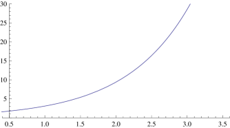
Figure 2: Plot of the solution to equation (4.43), where $z\in(0.4,3.4)$ and $Y\in(0.1,30)$. The parameters are $c_{1}=10,\epsilon=1,\phi=\pi/4,\sigma^{2}=0.02,~{}~{}d_{1}=0$.

5 Conclusion

We studied with the Lie group analysis the general equation (1.7) and obtain the three dimensional symmetry algebra $L_{3}$ (3.21). Using the Lie algebra $L_{3}$ and the corresponding optimal system of subalgebras we provide the complete set of non-equivalent reductions of the PDE (1.7) to ODEs. The reductions are listed in Table 2.

In addition we were able to figure out all possible forms of the function $g(\alpha)$ for which equation (1.7) admits an extension of the symmetry algebra $L_{3}$. All such functions are listed in (3.22)-(3.24). From the three equations with the special form of the function $g(\alpha)$ two equations were deduced earlier by different authors [10], [15] and studied with the Lie group analysis in [4]-[8]. The new equation in this list is equation (2.13) which corresponds to the function $g(\alpha)$ (3.23). The main properties of the symmetry algebra $L_{4}$ for this equation are represented in Theorem 4.1. The invariant reductions of (2.13) are described and studied in section 4. Using, similar to the general case, an optimal system of subalgebras we describe the complete set of non-equivalent reductions of the PDE to different ODEs. In all these cases we are able to solve the ODEs and obtain solutions in exact form. We skipped in one case the exact formula because it is too voluminous.

It is interesting to remark that the models (2.10), (2.16) and (2.13) where introduced under different finance-economical assumptions. Now we clarified how deep they are connected from mathematical point of view. Other interesting remark concerns the structure of the corresponding Lie algebras. The symmetry Lie algebras of the models (2.10), (2.16) and (2.13) are isomorphic. It is easy to understand because of all of them are solutions to the same determining system (3.19). Less evident is why the Lie algebra admitted by the risk-adjusted pricing methodology model studied in [3] is also isomorphic to the previous ones. It seems that many of the pricing options models in illiquid markets posses similar algebraic properties.

References

• [1] Bank, P. and Baum, D. : Hedging and portfolio optimization in financial markets with a large trader, Mathematical Finance 14(1) 1 – 18 (2004)
• [2] Belinfante, J.Β G.Β F. and Kolman B.: A survey of Lie groups and Lie algebras with applications and computational methods, Society for Industrial and Applied Lie mathematics, Philadelphia (1989)
• [3] Bordag, L.Β A.: Study of the risk-adjusted pricing methodology model with methods of Geometrical Analysis, arXiv:0911.0113v1, accepted in Stochastics: An Intenational Journal of Probability and Stochastical Processes, DOI: 10.1080/17442508.2010.489642,(2010)
• [4] Bordag, L.Β A.: Pricing options in illiquid markets: optimal systems, symmetry reductions and exact solutions, Lobachevskyi Journal of Mathematics, 31 (2) 90–99 (2010)
• [5] Bordag, L.Β A.: Symmetry reductions and exact solutions for nonlinear diffusion equations, International Journal of Modern Physics, 24(08–09) 1713–1716 (2009)
• [6] Bordag, L.Β A.: On option-valuation in illiquid markets: invariant solutions to a nonlinear model. In: Sarychev A., Shiryaev, A., Guerra M. and Grossinho M.Β R. (eds), Mathematical Control Theory and Finance, pp. 1–18. Springer, (2008)
• [7] Bordag, L.Β A. and Frey, R.: Pricing options in illiquid markets: symmetry reductions and exact solutions. In: Ehrhardt, M. (ed), Nonlinear Models in Mathematical Finance, pp. 103–130. Nova Science Publishers, New York (2009)
• [8] Bordag, L.Β A. and Chmakova, A.Β Y.: Explicit solutions for a nonlinear model of financial derivatives, International Journal of Theoretical and Applied Finance (IJTAF) 10(1) 1 – 21 (2007)
• [9] Delbaen, F. and Schachermayer, W.: The Mathematics of Arbitrage, Springer, Springer Finance, Berlin–Heidelberg (2006)
• [10] Frey, R. Perfect option replication for a large trader, Ph.D. thesis, ETH, Zurich (1996)
• [11] Ibragimov, N.Β H.: Lie group analysis of differential equations, CRS Press, Boca Raton (1994)
• [12] Karatzas, I. and Shreve, S.Β E.: Methods of mathematical finance, Springer, New York (1998)
• [13] Mikaelyan, A.: Analytical study of the SchΓΆnbucher-Wilmott model of the feedback effect of hedging in illiquid markets, Halmstad University, Technical Report IDE0914, Sweden, Halmstad (2009)
• [14] SchΓΆnbucher, P.Β J. and Willmott, P.: The Feedback effect of hedging in illiquid markets, SIAM Journal of Applied Mathematics 61(1) 232 – 272 (2000)
• [15] Sircar, K.Β R. and Papanicolaou, G.: General Black–Scholes models accounting for increased market volatility from hedging strategies, Applied Mathematics Finance 5 48 – 52 (1998)
• [16] Olver, P. J.: Applications of Lie groups to differential equations, Springer, New York (1993)
• [17] Ovsiannikov, L.Β V.: Group analysis of differential equations, Academic Press, New York (1982)
• [18] Patera, J. and Winternitz, P.: Subalgebras of real three- and four-dimensional Lie algebras, Journal of Mathematical Physics18(7) 1449 – 1455 (1977)
• [19] Stephani, H.: Differential equations. Their solution using symmetries, Cambridge University Press, Cambridge (1989)