The complete conformal spectrum of a $sl(2|1)$ invariant network model and logarithmic corrections

Abstract

We investigate the low temperature asymptotics and the finite size spectrum of a class of Temperley-Lieb models. As reference system we use the spin-1/2 Heisenberg chain with anisotropy parameter $\Delta$ and twisted boundary conditions. Special emphasis is placed on the study of logarithmic corrections appearing in the case of $\Delta=1/2$ in the bulk susceptibility data and in the low-energy spectrum yielding the conformal dimensions. For the $sl(2|1)$ invariant 3-state representation of the Temperley-Lieb algebra with $\Delta=1/2$ we give the complete set of scaling dimensions which show huge degeneracies.

1 Introduction

Many different, and at first sight unrelated physical phenomena like the thermodynamics of quantum spin chains, critical properties of two-dimensional classical vertex models and of supersymmetric network models are related on fundamental mathematical grounds. Often, such relations are established by mappings of quantum systems to classical systems, where the related objects are operators like the Hamiltonian and the transfer matrix ‘living’ in the same Hilbert space of physical states. Sometimes, the relations are less obvious as the related objects are defined in rather different spaces, but turn out to be equivalent representations of some underlying algebraic structure. The structure relevant to our investigations is the so-called Temperley-Lieb algebra [2, 1, 3]. The seminal model for correlated quantum many-body systems and the standard reference model of the Temperley-Lieb algebra is the well-known Heisenberg model. In one spatial dimension the system with nearest-neighbour exchange is exactly solvable for the spin-1/2 case [4]. Despite the integrability a comprehensive theoretical treatment is still missing. A notorious problem is posed by the calculation of correlation functions even at zero temperature, not to mention the corresponding properties at finite temperature. However, the asymptotics of the correlations in particular in the ground-state and at low temperatures are quite well understood by a combination of Bethe ansatz [1] and conformal field theory [5, 6]. At exactly zero temperature the spin-1/2 Heisenberg chain shows algebraic decay in its correlation functions and thereby constitutes a quantum critical system. Recently, the special point $\Delta=1/2$ of the anisotropic version of the Heisenberg chain, the so-called spin-1/2 $XXZ$ chain, has attracted strong interest as certain mathematical simplifications occur in the construction of the eigenstates [7, 8, 9]. Also its classical counterpart, the six-vertex model with suitable boundary conditions, allowed for new insight into many combinatorial problems like for instance the alternating sign matrices and boxed plane partitions, see e.g. [10, 11] and references therein. In the case $\Delta=1/2$ like for other special points, the so-called roots of unity of the $XXZ$ chain, a crossover of critical exponents leads to logarithmic corrections to the dominant critical behaviour. A notable case is the isotropic model $\Delta=1$ with logarithmic corrections to the low-temperature asymptotics, in particular for the susceptibility[12]. For the case $\Delta=1/2$ strong logarithmic corrections to the boundary susceptibility were found in [13]. In this paper we report on a low-temperature analysis of the $\Delta=1/2$ bulk properties that reproduce and confirm some of the findings in [25, 13]. The main motivation of this analysis is the applicability to the study of all low-lying excitations of the $XXZ$ chain with arbitrary twisted boundary condition allowing to calculate the energy levels beyond the conformal field theoretical results. The feasibility of such calculations is interesting because of applications to statistical mechanical models of the spin quantum Hall transition [14, 15, 16]. The localization-delocalization exponent was calculated in [16] from the mapping onto the two-dimensional percolation problem. The underlying system is a supersymmetric realization of the Temperley-Lieb algebra. Another model for describing the spin quantum Hall transition was introduced in [15] and investigated extensively in [17], however, still leaving open important questions. One of those questions concerns the relation of the two models. For the network model [16] the complete classification of the excited states resp. the scaling dimensions was performed by a Coulomb gas analysis in [33]. A combinatorial analysis based on a decomposition of the partition function for the Potts model on finite tori in terms of generalised characters can be found in [34]. Here we present a systematic representation theoretical analysis of the eigenvalues of the Temperley-Lieb Hamiltonian corresponding to the network model on finite chains with periodic and $\pi$-twisted boundary conditions. Our analysis is based on [35] where a Temperley-Lieb equivalence with particular emphasis on the boundary conditions was established for vertex-models. The precise mapping of the generic irreducible sub-representations of Temperley-Lieb Hamiltonians with periodic boundary conditions to the Heisenberg chain with suitable twisted boundary conditions allows for the determination of critical properties. Also in [35], the multiplicities of the sub-representations were worked out. The gained knowledge of the complete spectrum allowed for the computation of the thermodynamics of the Hamiltonians. In Section 2 of this paper an approach to the thermodynamics of the Heisenberg chain on the basis of non-linear integral equations for just two auxiliary functions is analysed [21] (see also the related approaches by [22, 23, 24]). For $\Delta=1/2$ an analytical calculation of the leading universal terms to the free energy and the magnetic susceptibility as well as the next-leading logarithmic corrections is presented. In Section 3 we study the critical exponents of correlation functions at zero temperature. The leading conformal finite-size spectrum of the Heisenberg chain with twisted boundary conditions and the next-leading correction terms in the case $\Delta=1/2$ beyond the CFT results are derived. In Section 4 we address the supersymmetric network model and calculate the complete set of scaling dimensions as well as their multiplicities and logarithmic corrections.

2 Thermodynamics and logarithmic corrections

We investigate the thermodynamical properties of the antiferromagnetic isotropic spin-1/2 Heisenberg chain

$$H=2J\sum_{j=1}^{L}[S_{j}^{x}S_{j+1}^{x}+S_{j}^{y}S_{j+1}^{y}+\Delta S_{j}^{z}S_{j+1}^{z}]$$ (1)

with anisotropy parameter $\Delta=\cos\gamma$ where $\gamma(\Delta=1/2)=\pi/3$. We note that the elementary excitations (‘spinons’) have quasi-linear energy-momentum dispersion with velocity

$$v=J\pi\frac{\sin\gamma}{\gamma}\to_{\Delta=1/2}\frac{3\sqrt{3}}{2}J.$$ (2)

The free energy per lattice site of the system is given by the following set of non-linear integral equations [21] for auxiliary functions $\mathfrak{a}$, and $\mathfrak{A}=1+\mathfrak{a}$

$$\log\mathfrak{a}(x)=-\frac{v\beta}{\cosh x}+\phi+\int_{-\infty}^{\infty}\left[k(x-y)\log\mathfrak{A}(y)-k(x-y-i\pi+i\epsilon)\log\overline{\mathfrak{A}}(y)\right]{\rm d}y,$$ (3)

and the corresponding equation for $\overline{{\mathfrak{a}}}$, and $\overline{{\mathfrak{A}}}=1+\overline{{\mathfrak{a}}}$ are related to (3) by ‘complex conjugation’, in particular by exchanging $\mathfrak{a}\leftrightarrow\overline{{\mathfrak{a}}}$, and by changing the sign of $\phi\leftrightarrow-\phi$ though being real as given by the external magnetic field $\phi=\frac{\pi\beta h}{2(\pi-\gamma)}\to_{\Delta=1/2}\frac{3}{4}\beta h$. The integration kernel is defined by the Fourier integral

$$k(x)=\frac{1}{2\pi}\int_{-\infty}^{\infty}\frac{\sinh\left(\frac{\pi}{\gamma}-2\right)\frac{\pi}{2}k}{2\cosh\frac{\pi}{2}k\sinh\left(\frac{\pi}{\gamma}-1\right)\frac{\pi}{2}k}\cos(kx)dk\to_{\Delta=1/2}\frac{1}{2\pi^{2}}\frac{x}{\sinh x}.$$ (4)

In terms of the solution $\mathfrak{A}$ and $\overline{{\mathfrak{A}}}$ to the integral equations the free energy is given by

$$\beta f=\beta e_{0}-\frac{1}{2\pi}\int_{-\infty}^{\infty}\frac{\log[\mathfrak{A}\overline{{\mathfrak{A}}}(x)]}{\cosh x}dx.$$ (5)

These equations are readily solved numerically for arbitrary fields and temperatures by utilizing the difference type of the integral kernel and Fast Fourier Transform. In Figs. 1 and 2 the results for the specific heat and susceptibility are shown for zero external magnetic field. At low temperatures the specific heat shows linear asymptotics $c(T)\simeq\frac{\pi c}{3v}T$ with velocity of the elementary excitations $v$ and central charge $c=1$. The zero temperature limit of the susceptibility is $\chi_{0}=1/(2v(\pi-\gamma))$.

Figure 1: Specific heat $c(T)$ data versus temperature $T$ ($J=1$) for the spin-1/2 $XXZ$ chain with anisotropy $\Delta=0,0.5,1$ and zero field $h=0$.

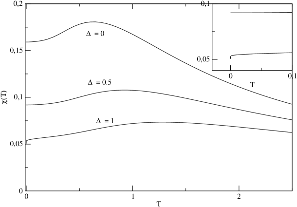
Figure 2: Susceptibility $\chi(T)$ data versus temperature $T$ ($J=1$) for the spin-1/2 $XXZ$ chain with anisotropy $\Delta=0,0.5,1$ and zero field $h=0$. In the inset the low temperature behaviour of $\chi(T)$ for $\Delta=0.5$ and $1$ is shown.

For $\Delta=1$ there are logarithmic corrections to the susceptibility $\chi(T)$ at low temperatures as noticed in [12, 20] and to the specific heat $c(T)$. For a detailed analysis of the isotropic point we refer the reader to [12, 25, 28]. We like to point out that already for moderately low temperatures the correction terms are noticeable for $\chi(T)$, see Fig. 2. There are other cases of the anisotropy parameter $\Delta$ with logarithmic corrections at low temperatures. One of these cases is $\Delta=1/2$ as noticed and analysed in [25, 13]. Already a glance to Fig. 2 suggests that these correction terms must be of higher, i.e. less leading, order. Here we like to present a completely analytical low-temperature analysis (for $h<<T$) for the case $\Delta=1/2$ from the non-linear integral equations. With view to the asymptotical properties of the driving term on the RHS of (3) it is convenient to introduce the following scaling functions

$${\mathfrak{a}}^{+}_{\mathfrak{L}}(x) = \mathfrak{a}(x+{\mathfrak{L}}),\qquad{\mathfrak{L}}:=\ln(v\beta),$$

$${\mathfrak{a}}^{-}_{\mathfrak{L}}(x) = \mathfrak{a}(-x-{\mathfrak{L}}),$$ (6)

approaching well-defined non-trivial limiting functions in the low-temperature limit which satisfy

$$\log{\mathfrak{a}}^{+}_{\mathfrak{L}}(x) = -2{\rm e}^{-x}+O\left({1}/{\beta^{2}}\right)+\phi+\psi_{\mathfrak{L}}(x)$$ (7)

$$+\int_{-{\mathfrak{L}}}^{\infty}\left[k(x-y)\log{\mathfrak{A}}^{+}_{\mathfrak{L}}(y)-k(x-y-i\pi+i\epsilon)\log\overline{{\mathfrak{A}}}^{+}_{\mathfrak{L}}(y)\right]{\rm d}y,$$

where $\psi_{\mathfrak{L}}(x)$ accounts for the contribution of the functions $\mathfrak{A}$ and $\overline{{\mathfrak{A}}}$ on the negative real axis

$$\psi_{\mathfrak{L}}(x)=\int_{-{\mathfrak{L}}}^{\infty}\left[k(x+y+2{\mathfrak{L}})\log{\mathfrak{A}}^{-}_{\mathfrak{L}}(y)-k(x+y+2{\mathfrak{L}}-i\pi+i\epsilon)\log\overline{{\mathfrak{A}}}^{-}_{\mathfrak{L}}(y)\right]{\rm d}y.$$ (8)

Using these functions the free energy at low temperatures takes the form

$$f=e_{0}-\frac{1}{\pi v\beta^{2}}\int_{-{\mathfrak{L}}}^{\infty}{\rm e}^{-x}\log\left[{\mathfrak{A}}^{+}_{\mathfrak{L}}\overline{{\mathfrak{A}}}^{+}_{\mathfrak{L}}{\mathfrak{A}}^{-}_{\mathfrak{L}}\overline{{\mathfrak{A}}}^{-}_{\mathfrak{L}}(x)\right]dx+O\left(1/\beta^{4}\right).$$ (9)

In order to analyse the low-temperature asymptotics in detail we perform the following manipulation

$$\int_{-{\mathfrak{L}}}^{\infty}\left[(\log{\mathfrak{a}}^{+}_{\mathfrak{L}})^{\prime}(\log{\mathfrak{A}}^{+}_{\mathfrak{L}})-(\log{\mathfrak{a}}^{+}_{\mathfrak{L}})(\log{\mathfrak{A}}^{+}_{\mathfrak{L}})^{\prime}\right]dx+\hbox{`conj'},$$

$$=\int_{-{\mathfrak{L}}}^{\infty}\left[(-2{\rm e}^{-x}+\phi+\psi_{\mathfrak{L}}(x))^{\prime}(\log{\mathfrak{A}}^{+}_{\mathfrak{L}})-(-2{\rm e}^{-x}+\phi+\psi_{\mathfrak{L}}(x))(\log{\mathfrak{A}}^{+}_{\mathfrak{L}})^{\prime}\right]dx+\hbox{`conj'},$$

$$=2\int_{-{\mathfrak{L}}}^{\infty}(2{\rm e}^{-x}+\psi_{\mathfrak{L}}(x)^{\prime})(\log{\mathfrak{A}}^{+}_{\mathfrak{L}})dx-\phi\log\left(1+{\rm e}^{\frac{4}{3}\phi}\right)+\hbox{`conj'},$$ (10)

where in the second line we have inserted (7) and used the symmetry of the integration kernel ($k_{ij}(x)=k_{ji}(-x)$ where indices 1 and 2 refer to functions $\mathfrak{a}$, $\mathfrak{A}$ and $\overline{{\mathfrak{a}}}$, $\overline{{\mathfrak{A}}}$ respectively). In the third line we have performed an integration by parts with an explicit evaluation of the contribution by the integral terminals using the limits

$$\log{\mathfrak{a}}^{+}_{\mathfrak{L}}(\infty) = {+\frac{4}{3}\phi},\qquad\log{\mathfrak{A}}^{+}_{\mathfrak{L}}(\infty)=\log\left(1+{\rm e}^{+\frac{4}{3}\phi}\right),$$

$$\log\overline{{\mathfrak{a}}}^{+}_{\mathfrak{L}}(\infty) = {-\frac{4}{3}\phi},\qquad\log\overline{{\mathfrak{A}}}^{+}_{\mathfrak{L}}(\infty)=\log\left(1+{\rm e}^{-\frac{4}{3}\phi}\right).$$ (11)

Next, we show that the LHS of (10) can be evaluated explicitly as it is a definite integral of dilogarithmic type with known terminals

$$LHS = 2\int_{-{\mathfrak{L}}}^{\infty}(\log{\mathfrak{a}}^{+}_{\mathfrak{L}})^{\prime}\log{\mathfrak{A}}^{+}_{\mathfrak{L}}dx-\log{\mathfrak{a}}^{+}_{\mathfrak{L}}\log{\mathfrak{A}}^{+}_{\mathfrak{L}}\Big{|}_{-{\mathfrak{L}}}^{\infty}+\hbox{`conj'},$$ (12)

$$= 2\int_{-\infty}^{4\phi/3}\log(1+{\rm e}^{z})dz-\frac{4}{3}\phi\log(1+{\rm e}^{\frac{4}{3}\phi})+2\int_{-\infty}^{-4\phi/3}\log(1+{\rm e}^{z})dz+\frac{4}{3}\phi\log(1+{\rm e}^{-\frac{4}{3}\phi}),$$

$$= \frac{\pi^{2}}{3},$$

where the second line is independent of $\phi$ (to be checked by differentiation) and the particular choice $\phi=0$ ‘directly’ leads to the last line. From the general expression (5) of the free energy $f$ in terms of the functions $\mathfrak{A}$ and $\overline{{\mathfrak{A}}}$ the detailed functional dependence of $\mathfrak{A}$ and $\overline{{\mathfrak{A}}}$ on the argument matters even for the calculation of the asymptotic behaviour of $f$ at low temperature. The usefulness of (10) lies in the fact that the integral of interest is related to another integral where only the asymptotic behaviour of $\mathfrak{A}$ and $\overline{{\mathfrak{A}}}$ at large spectral parameter enters. Combining (10) and (12) we arrive at a formula particularly suited for studying the asymptotic behaviour of (9)

$$4\int_{-{\mathfrak{L}}}^{\infty}{\rm e}^{-x}\log[{\mathfrak{A}}^{+}_{\mathfrak{L}}\overline{{\mathfrak{A}}}^{+}_{\mathfrak{L}}]dx=\frac{\pi^{2}}{3}+\frac{4}{3}\phi^{2}-2\int_{-{\mathfrak{L}}}^{\infty}\left[\psi_{\mathfrak{L}}(x)^{\prime}\log{\mathfrak{A}}^{+}_{\mathfrak{L}}+\overline{\psi}_{\mathfrak{L}}(x)^{\prime}\log\overline{{\mathfrak{A}}}^{+}_{\mathfrak{L}}\right]dx.$$ (13)

The first term on the right hand side determines the leading $O(T^{2})$ term of the free energy, see (9), the remaining integral is a higher order term which can be calculated by explicit use of special properties of the integral kernel (4), especially the asymptotic behaviour

$$k(x)\simeq\frac{1}{\pi^{2}}x\,{\rm e}^{-x}.$$ (14)

This allows to approximate (8) by

$$\psi_{\mathfrak{L}}(x)\simeq\overline{\psi}_{\mathfrak{L}}(x)\simeq\int_{-{\mathfrak{L}}}^{\infty}k(x+y+2{\mathfrak{L}})\log\left[{\mathfrak{A}}^{-}_{\mathfrak{L}}(y)\overline{{\mathfrak{A}}}^{-}_{\mathfrak{L}}(y)\right]{\rm d}y,$$ (15)

leading to a symmetric double integral

$$\int_{-{\mathfrak{L}}}^{\infty}\left[\psi_{\mathfrak{L}}(x)^{\prime}\log{\mathfrak{A}}^{+}_{\mathfrak{L}}(x)+\overline{\psi}_{\mathfrak{L}}(x)^{\prime}\log\overline{{\mathfrak{A}}}^{+}_{\mathfrak{L}}(x)\right]dx$$

$$\simeq\int_{-{\mathfrak{L}}}^{\infty}\int_{-{\mathfrak{L}}}^{\infty}\log\left[{\mathfrak{A}}^{+}_{\mathfrak{L}}(x)\overline{{\mathfrak{A}}}^{+}_{\mathfrak{L}}(x)\right]k^{\prime}(x+y+2{\mathfrak{L}})\log\left[{\mathfrak{A}}^{-}_{\mathfrak{L}}(y)\overline{{\mathfrak{A}}}^{-}_{\mathfrak{L}}(y)\right]{\rm d}y{\rm d}x$$

$$\simeq-\frac{2{\mathfrak{L}}}{\pi^{2}}{\rm e}^{-2{\mathfrak{L}}}\left(\int_{-{\mathfrak{L}}}^{\infty}{\rm e}^{-x}\log\left[{\mathfrak{A}}^{+}_{\mathfrak{L}}(x)\overline{{\mathfrak{A}}}^{+}_{\mathfrak{L}}(x)\right]{\rm d}x\right)\left(\int_{-{\mathfrak{L}}}^{\infty}{\rm e}^{-y}\log\left[{\mathfrak{A}}^{-}_{\mathfrak{L}}(y)\overline{{\mathfrak{A}}}^{-}_{\mathfrak{L}}(y)\right]{\rm d}y\right).$$ (16)

Amazingly, the integrals in the final version are those we calculated already in leading order

$$\left(\int_{-{\mathfrak{L}}}^{\infty}{\rm e}^{-x}\log[{\mathfrak{A}}^{+}_{\mathfrak{L}}\overline{{\mathfrak{A}}}^{+}_{\mathfrak{L}}]dx\right)_{\infty}=\frac{1}{4}\left(\frac{\pi^{2}}{3}+\frac{4}{3}\phi^{2}\right).$$ (17)

Hence

$$\int_{-{\mathfrak{L}}}^{\infty} {\rm e}^{-x} \log[{\mathfrak{A}}^{+}_{\mathfrak{L}}\overline{{\mathfrak{A}}}^{+}_{\mathfrak{L}}]dx$$ (18)

$$\simeq \left(\int_{-{\mathfrak{L}}}^{\infty}{\rm e}^{-x}\log[{\mathfrak{A}}^{+}_{\mathfrak{L}}\overline{{\mathfrak{A}}}^{+}_{\mathfrak{L}}]dx\right)_{\infty}-\frac{1}{2}\int_{-{\mathfrak{L}}}^{\infty}\left[\psi_{\mathfrak{L}}(x)^{\prime}\log{\mathfrak{A}}^{+}_{\mathfrak{L}}+\overline{\psi}_{\mathfrak{L}}(x)^{\prime}\log\overline{{\mathfrak{A}}}^{+}_{\mathfrak{L}}\right]dx,$$

$$\simeq \left(\int_{-{\mathfrak{L}}}^{\infty}{\rm e}^{-x}\log[{\mathfrak{A}}^{+}_{\mathfrak{L}}\overline{{\mathfrak{A}}}^{+}_{\mathfrak{L}}]dx\right)_{\infty}$$

$$+\frac{{\mathfrak{L}}}{\pi^{2}}{\rm e}^{-2{\mathfrak{L}}}\left(\int_{-{\mathfrak{L}}}^{\infty}{\rm e}^{-x}\log\left[{\mathfrak{A}}^{+}_{\mathfrak{L}}(x)\overline{{\mathfrak{A}}}^{+}_{\mathfrak{L}}(x)\right]{\rm d}x\right)\left(\int_{-{\mathfrak{L}}}^{\infty}{\rm e}^{-y}\log\left[{\mathfrak{A}}^{-}_{\mathfrak{L}}(y)\overline{{\mathfrak{A}}}^{-}_{\mathfrak{L}}(y)\right]{\rm d}y\right).$$

The final result reads

$$\int_{-{\mathfrak{L}}}^{\infty}{\rm e}^{-x}\log[{\mathfrak{A}}^{+}_{\mathfrak{L}}\overline{{\mathfrak{A}}}^{+}_{\mathfrak{L}}]dx\simeq\frac{1}{4}\left(\frac{\pi^{2}}{3}+\frac{4}{3}\phi^{2}\right)+\frac{{\mathfrak{L}}}{16\pi^{2}}{\rm e}^{-2{\mathfrak{L}}}\left(\frac{\pi^{2}}{3}+\frac{4}{3}\phi^{2}\right)^{2}$$ (19)

implying logarithmic corrections in $T$ for the free energy and the zero-field susceptibility

$$f \simeq e_{0}-\frac{T^{2}}{2\pi v}\left(\left(\frac{\pi^{2}}{3}+\frac{4}{3}\phi^{2}\right)+\frac{{\mathfrak{L}}}{4\pi^{2}}{\rm e}^{-2{\mathfrak{L}}}\left(\frac{\pi^{2}}{3}+\frac{4}{3}\phi^{2}\right)^{2}\right)\quad{\mathfrak{L}}=\ln(v/T),\quad(h<<T),$$ (20)

$$\simeq e_{0}-\frac{\pi}{6v}T^{2}\left(1+\left(2\phi/\pi\right)^{2}\right)\left(1+\frac{T^{2}\ln(v/T)}{12v^{2}}\left(1+\left(2\phi/\pi\right)^{2}\right)\right),$$

$$\chi = \frac{3}{4\pi v}\left(1+\frac{2T^{2}\ln(v/T)}{3^{4}J^{2}}\right).$$ (21)

This result is in complete agreement with the effective Hamiltonian analysis of [25, 13] where also higher order terms were calculated. In this approach, the occurence of the logarithmic correction stems from the interference of the first-order contribution of the $T\bar{T}$ perturbation to the Gaussian Hamiltonian with the second-order contribution of the cosine of the bosonic fields. The main motivation of our analysis is not the systematic extension of the low temperature corrections. We intend to compute the entire low-lying excitation spectrum of the quantum transfer matrix and by the $\beta\leftrightarrow L$ correspondence the spectrum of the Hamiltonian up to order $1/L$ and $(\ln L)/L^{3}$.

3 Critical indices and low-lying eigenvalues of the Heisenberg chain

A major area of interest in statistical physics is the study of critical properties of models at phase transitions and, more specifically, the determination of the scaling dimensions $x$, from which the critical exponents can be deduced. For the critical two-dimensional six-vertex model and the associated spin-1/2 $XXZ$ quantum chain a wealth of information has been collected by combinations of finite size studies of the eigenvalue spectrum and scaling relations by conformal field theory. The energy levels of the corresponding quantum model on a finite chain with periodic boundary conditions scale with the system size $L$ like (see [6] and references therein)

$$E_{x}-E_{0}=\frac{2\pi}{L}vx+o\left(\frac{1}{L}\right),\qquad E_{0}=Le_{0}-\frac{\pi v}{6L}c,$$ (22)

where $E_{0}$ is the ground state energy, $E_{x}$ are the energies of the low-lying excited states and $v$ is the sound velocity of the elementary energy-momentum excitations. Equivalent formulae can be set up for the spectrum of the row-to-row transfer matrix of the two-dimensional model. For the critical six-vertex model the scaling dimensions have been treated by analytical as well as numerical methods based on (22). The dimensions $x$ are given by the Gaussian spectrum [29, 30, 31]. The analytic method for calculating finite-size corrections based on linear integral equations for density functions of Bethe ansatz rapidities was applied to many models. However, this method has the shortcoming that it fails for the higher spin-$S$ $XXZ$ chains and similar problems. There is an alternative procedure based on non-linear integral equations (NLIE) for suitably chosen auxiliary functions which proved to be applicable also in the hitherto problematic cases of higher spin-$S$ chains, i.e. for systems supporting filled seas of string configurations. At the same time the NLIE method proved flexible enough [32] to give a comprehensive analytical study of the six-vertex model spectrum. The eigenvalues are obtained from non-linear integral equations [21] for auxiliary functions $\mathfrak{a}$, and $\mathfrak{A}=1+\mathfrak{a}$

$$\log\mathfrak{a}(x)=L\ln\tanh\frac{x}{2}+C+\int_{-\infty}^{\infty}\left[k(x-y)\log\mathfrak{A}(y)-k(x-y-i\pi+i\epsilon)\log\overline{\mathfrak{A}}(y)\right]{\rm d}y,$$ (23)

and the corresponding equation for $\overline{{\mathfrak{a}}}$, and $\overline{{\mathfrak{A}}}=1+\overline{{\mathfrak{a}}}$ related by complex conjugation. These equations are very similar to those in (3). The only difference is the change in the driving term

$$-\frac{v\beta}{\cosh x}\leftrightarrow L\ln\tanh\frac{x}{2}.$$ (24)

Note that the asymptotics of both functions are the same exponentials with different prefactors: $-2v\beta\exp(-x)$ and $-2L\exp(-x)$. The constant $C$ in (23) is $i\pi\varphi/(\pi-\gamma)$ where $\varphi$ is the twist angle of the generalized periodic boundary conditions. (For certain excited states, the constant $C$ may take different values.) The energy corresponding to a solution to the NLIE (23) satisfies an integral expression very similar to (5). Therefore the analysis of the finite size Hamiltonian can be carried out very closely to the analysis of the low-temperature analysis of the previous section. The main results for the general $XXZ$ chain were obtained already in [32] and may be summarized for the $1/L$ contributions to the energy and momentum eigenvalues as

$$\frac{L}{2\pi v}(E-Le_{0})=-\frac{1}{2\pi^{2}}\left(\int_{-{\mathfrak{L}}}^{\infty}{\rm e}^{-x}\log\left[{\mathfrak{A}}^{+}_{\mathfrak{L}}\overline{{\mathfrak{A}}}^{+}_{\mathfrak{L}}(x)\right]dx+\int_{-{\mathfrak{L}}}^{\infty}{\rm e}^{-x}\log\left[{\mathfrak{A}}^{-}_{\mathfrak{L}}\overline{{\mathfrak{A}}}^{-}_{\mathfrak{L}}(x)\right]dx\right),$$

$$\frac{L}{2\pi}P=-\frac{1}{2\pi^{2}}\left(\int_{-{\mathfrak{L}}}^{\infty}{\rm e}^{-x}\log\left[{\mathfrak{A}}^{+}_{\mathfrak{L}}\overline{{\mathfrak{A}}}^{+}_{\mathfrak{L}}(x)\right]dx-\int_{-{\mathfrak{L}}}^{\infty}{\rm e}^{-x}\log\left[{\mathfrak{A}}^{-}_{\mathfrak{L}}\overline{{\mathfrak{A}}}^{-}_{\mathfrak{L}}(x)\right]dx\right).$$ (25)

These formulae have a rather universal algebraic form as they are valid for all eigenvalues of the Hamiltonian with suitably chosen contours! In [32] the leading contribution to the integrals was calculated

$$\int_{-{\mathfrak{L}}}^{\infty}{\rm e}^{-x}\log\left[{{\mathfrak{A}}^{\pm}_{\mathfrak{L}}}{\overline{{\mathfrak{A}}}^{\pm}_{\mathfrak{L}}}(x)\right]dx=-{2\pi^{2}}\left(\frac{x(\varphi)\pm s(\varphi)}{2}-\frac{1}{24}\right)$$ (26)

where

$$x(\varphi) = x_{S,m}(\varphi)=\frac{1-\gamma/\pi}{2}S^{2}+\frac{1}{2(1-\gamma/\pi)}\left(m-\frac{\varphi}{\pi}\right)^{2}$$

$$s(\varphi) = S\left(m-\frac{\varphi}{\pi}\right)$$ (27)

are the ‘scaling dimension’ and ‘conformal spin’, and $S$ and $m$ are integers. From these results with $S=m=0$ and (22) also the (effective) central charge follows

$$c(\varphi)=1-\frac{6(\varphi/\pi)^{2}}{1-\gamma/\pi}$$ (28)

For the special case of interest ($\Delta=1/2$) we are able to calculate the next leading contribution to the integrals on the right hand side of (25). We note that (18) holds with the result

$$\int_{-{\mathfrak{L}}}^{\infty}{\rm e}^{-x}\log\left[{{\mathfrak{A}}^{\pm}_{\mathfrak{L}}}{\overline{{\mathfrak{A}}}^{\pm}_{\mathfrak{L}}}(x)\right]dx=\pi^{2}\left[1/{12}-(x(\varphi)\pm s(\varphi))\right]+\pi^{2}{{\mathfrak{L}}}{\rm e}^{-2{\mathfrak{L}}}\left[(1/{12}-x(\varphi))^{2}-s^{2}(\varphi))\right],$$ (29)

where now

$${\mathfrak{L}}=\ln L\Rightarrow{{\mathfrak{L}}}{\rm e}^{-2{\mathfrak{L}}}=\frac{\ln L}{L^{2}}.$$ (30)

These relations imply that the next-leading corrections over the ($1/L$) conformal field theory results for the energy levels are

$$E_{x}-E_{x}^{CFT}=-2\pi v\left[(1/{12}-x(\varphi))^{2}-s^{2}(\varphi))\right]\frac{\ln L}{L^{3}},$$ (31)

where $v$ is the velocity of the elementary excitations. Our results agree with those of [25] and (slightly) generalize them to arbitrary twisted boundary conditions.

4 The $sl(2|1)$-invariant network model: Temperley-Lieb representation with $\Delta=1/2$

Here we investigate the critical properties of the statistical mechanical network model derived in [14, 16] for the spin quantum Hall transition which may occur in disordered superconductors with unbroken $SU(2)$ spin-rotation symmetry but broken time-reversal symmetry [18]. Using supersymmetry, and averaging over the random $SU(2)$ matrices a classical 3-state model on the square lattice was derived with local Boltzmann weights resp. the $R$-matrix given as a superposition of the identity and the projector onto the $sl(2|1)$-singlet state of nearest-neighbours. Thus, the study of the localization-delocalization transition was mapped onto the two-dimensional percolation problem. Furthermore, the local Boltzmann weights derived in [16] are a realization of the Temperley-Lieb algebra [2, 1, 3] and hence the model is related to some (inhomogeneous) six-vertex model. For the symmetric case, the network model in [16] is related to an integrable homogeneous six-vertex model. In our representation theoretical treatment we give the identification of the type of boundary conditions to be used for the six-vertex model which is essential for the determination of the scaling dimensions in a finite-size analysis of eigenvalues of transfer matrices and/or Hamiltonians. The Temperley-Lieb algebra $TL(\lambda)$ is the unital associative algebra over $\mathbb{C}$ generated by $e_{1},\,e_{2},\,\dots,e_{L-1}$ with relations

$$\begin{split}e_{i}^{2}=&\;\lambda\;e_{i},\\ e_{i}\;e_{j}\;e_{i}=&\;e_{i},\;\;\;\mbox{if}\ i,j\ \mbox{nearest neighbours}\\ e_{i}\;e_{j}=&\;e_{j}\;e_{i},\;\;\;\mbox{if}\ i,j\ \mbox{not nearest neighbours}\end{split}$$ (32)

depending on the complex parameter $\lambda=2\Delta$, where $\Delta$ is the anisotropy parameter of the anisotropic Heisenberg chain which is the standard (faithful) representation of the Temperley-Lieb algebra. The periodic closure of $TL(\lambda)$ has one additional generator $e_{L}$ and relations (32) with 1 and $L$ beeing considered as neighbouring indices. For a full description of the periodic (and more generally twisted) closure we refer the reader to [35] and references therein. According to the realization of $TL(\lambda)$ as a diagram algebra we use the following graphical notation for the operators $e_{i}$:

$$e_{i} = \underbrace{~{}\psfig{width=56.9055pt}~{}}_{id^{\otimes(i-1)}}~{}\quad\psfig{width=28.45274pt}~{}\;\quad\underbrace{~{}\psfig{width=56.9055pt}~{}}_{id^{\otimes(L-i-1)}}$$ (33)

where the two curved links correspond to the bra- and ket-states of the local $sl(2|1)$ singlet. Obviously, the parameter $\lambda$ appearing in (32) has the counterpart of a closed loop which for the model in [16] is 1 ($=1-1+1$ due to the alternating standard and non-standard anti-commutation relations for fermions on odd and even lattice sites). These constructions may be generalized to the case of a $sl(n+1|n)$-invariant network model, again of Temperley-Lieb type with $\Delta=1/2$, but now with a total number of states per site $d=2n+1$. The statistical mechanical model of [16] has a staggered structure with two types of local Boltzmann weights alternating from row to row, cf. Fig. 3. The local Boltzmann weights can be given in terms of so-called $R$-matrices which are defined by

$$R_{j,j+1}(u):=\sin(\gamma-u)+\sin(u)e_{j}$$ (34)

where $\gamma=\pi/3$ and $u$ takes certain values $\Theta_{A}$ and $\Theta_{B}$ alternatingly from row to row.

Figure 3: Depiction of the Chalker-Coddington model. Each vertical zig-zag line corresponds to a local quantum space. Solid and dashed lines correspond to dual representations of $sl(2|1)$. In the general, inhomogeneous case, there are independent local interactions $R(\Theta_{A})$ and $R(\Theta_{B})$ on even and odd rows.

For general parameters $\Theta_{A,B}$ the model is not exactly solvable. However, for identical interaction parameters $\Theta:=\Theta_{A}=\Theta_{B}$, the row-to-row transfer matrices belong to a commuting family of transfer matrices defined on a square lattice with the same width and height as in Fig. 3 but with horizontal and vertical lines to which spectral parameters are associated. On the vertical lines we place alternatingly 0 and $\Theta$. Now consider a single row with spectral parameter $v$ attached to the horizontal line. The corresponding transfer matrix is denoted by $T(v)$ and consists of an alternating product of $R(v-0)$ and $R(v-\Theta)$ matrices, see Fig. 4 a). All matrices $T(v)$ with arbitrary complex argument $v$ commute due to the Yang-Baxter relation satisfied by (34). For $v=0$ the lattice in Fig. 3 is recovered. This is most easily understood by observing that $R(0)$ is proportional to the identity operator and $T(0)$ factors as shown in Fig. 4 b). The product of two transfer matrices $T(0)$, cf. Fig. 4 b), corresponds to two successive rows in Fig. 3 times a translation by two lattice units. For a lattice of square shape the translation operators reduce to the identity and the partition function of Fig. 3 is identical to $\textnormal{Tr}\big{[}T(0)^{L}\big{]}$.

Figure 4: a) Graphical depiction of a row-to-row transfer matrix $T(v)$ with spectral parameter $v$ associated with the horizontal line and alternatingly 0 and $\Theta$ associated with the vertical lines. Interactions are formulated for each vertex with local Boltzmann weight given by an $R$-matrix $R(u)$ where $u$ is taken as the difference of the two spectral parameters of the intersecting lines. This construction renders the transfer matrix integrable. Note the factorization taking place for $v=0$ at every second vertex as $R(0)$ reduces to the identity, a) and b).

Instead of working out the critical properties directly for the model depicted in Fig. 3 (with $\Theta=\Theta_{A}=\Theta_{B}$ we use the integrability of the transfer matrix $T(v)$. Due to the commutativity, the eigenstates of $T(v)$ are independent of $v$. The largest eigenvalue of $T(0)$ is realized by the eigenstate with the lowest eigenvalue of the corresponding Hamiltonian $H$. Note that also the product $T_{2}(v):=T(v)T(v+\Theta)$ is a commuting set of matrices generated by the complex variable $v$. For $v=0$ and by use of ‘unitarity’ for the $R$-matrix, this matrix can be shown to reduce to the translation operator by two lattice sites. The logarithmic derivative of $T_{2}(v)$ is nothing but

$$H=-\sum_{i=1}^{L}e_{i}$$ (35)

The critical properties of the system, e.g. correlation functions of local operators, are described by the scaling dimensions which are obtained from the finite-size data of the low-lying excitations of this Hamiltonian with periodic boundary conditions or with twist angle $\pi$. In the dense loop representation of the model, periodic boundary conditions render closed loops to evaluate to 1 (= number of bosonic states per site - number of fermionic states per site), for $\pi$-twisted boundary condition such loops evaluate to the total number of states per site $d$. As shown in [35] the sub-representations of the above Temperley-Lieb model appear as sub-representations in the standard reference Heisenberg chain, however with a new twist angle $\varphi$ appearing. The representations are constructed by attaching $k$-many singlets ($k\leq L/2$) to a pseudo-vacuum on a chain of length $N=L-2k$. The dimension of the space $\Omega_{N}^{p}$ of pseudo-vacua of length $N$ for periodic boundary conditions is given by (see appendix)

$$\mbox{dim}(\Omega_{N}^{p})(d)=\left(\frac{d}{2}+\frac{\sqrt{d^{2}-4}}{2}\right)^{N}+\left(\frac{d}{2}-\frac{\sqrt{d^{2}-4}}{2}\right)^{N},$$ (36)

which specializes for a 3-dimensional local Hilbert space to $\mbox{dim}(\Omega_{N}^{p})(3)=\left[(3+\sqrt{5})/2\right]^{N}+\left[(3-\sqrt{5})/2\right]^{N}$. In this space the translation operator shifting the system by two lattice sites can be diagonalized yielding momentum eigenvalues $P=l\cdot 2\pi/S$ where $l=0,...,S-1$ ($N=2S$). The energy eigenvalues of the Temperley-Lieb model in the sub-representation with $k$-many singlets and momentum $l\cdot 2\pi/S$ reference state are identical to those of the $XXZ$ quantum chain with $k$-many flipped spins (i.e. $L-k$ up and $k$ down spins with magnetization $S=N/2$) and twist angle

$$\varphi=\frac{P}{2}=l\cdot\frac{\pi}{S}.$$ (37)

Note that the dependence of the eigenvalues of the $XXZ$ reference system on $\varphi$ is $\pi$-periodic. The quantum number $l$ takes integer values for periodic and $\pi$-twisted boundary conditions of the Temperley-Lieb model, except for the $\pi$-twist and an odd number of fermions in the pseudo-vacuum. In such a case, the set of allowed values for $l$ is shifted by $1/2$ ($l=1/2,3/2,...,S-1/2$) which will not be pursued furthermore. The case $S=0$ ($k=L/2$, $N=0$) is special. Here the relation between the twist angles is given by equating macroscopic loops

$$1\mp 1+1={\rm e}^{i\varphi}+{\rm e}^{-i\varphi},$$ (38)

for periodic boundary conditions and $\pi$-twist. Explicitly we find

$$\varphi=\pi/3\quad\hbox{resp.}\quad i\ln\left((3+\sqrt{5})/2\right),$$ (39)

a real/imaginary value for periodic boundary conditions and $\pi$-twist. (For the general $sl(n+1|n)$ case, the left hand side in (38) is to be replaced by 1 or $d$ for periodic or $\pi$-twisted boundary conditions.) We read off the central charge from (28) with $\gamma=\pi/3$ and (39) as $c=0$ for periodic boundary conditions and $c=1+\left(\frac{3}{\pi}\ln\left[(3+\sqrt{5})/2\right]\right)^{2}$ for the $\pi$-twist. The scaling dimensions corresponding to low-lying excitations in the sub-representation with $k$-many singlets appended to a length $N$ pseudo-vacuum ($N=L-2k$) are obtained from (27)

$$x = \frac{L}{2\pi v}\left[E_{L}(\varphi)-E_{L,0}(\pi/3)\right]=\frac{L}{2\pi v}\left(\left[E_{L}(\varphi)-E_{L,0}(0)\right]-\left[E_{L}(\pi/3)-E_{L,0}(0)\right]\right)$$ (40)

$$= x_{S,m}(\varphi)-x_{0,0}(\pi/3)=\frac{4\,S^{2}+9(m-\varphi/\pi)^{2}-1}{12},$$ (41)

where the twist angle $\varphi$ is as in (37) and the true ground-state corresponds to $S=m=0$ and twist angle in (39). Next we give the multiplicities of the momentum values in the space $\Omega_{N}^{p}$ of all pseudo-vacua of length $N$ for periodic boundary conditions. First, the dimension of this space is (see appendix)

$$d(N):=\mbox{dim}(\Omega_{N}^{p})=\left(\frac{d}{2}+\frac{\sqrt{d^{2}-4}}{2}\right)^{N}+\left(\frac{d}{2}-\frac{\sqrt{d^{2}-4}}{2}\right)^{N}.$$ (42)

The subspace of $\Omega_{N}^{p}$ of states with an odd number of fermions has dimension (see appendix)

$$d^{o}(N)=\frac{d(N)}{2}-\cos\left(\frac{\pi}{3}N\right).$$ (43)

The eigenstates of the translation operator by two sites in $\Omega_{N}^{p}$ are constructed from the orbits with periods $p$ (which are divisors of $N$). Here we follow closely the treatment in [35], the main difference is that we now deal with a translation operator by two lattice sites and hence an orbit with period $p$ covers $2p$ sites. The dimensions of the orbits are denoted by $\sigma(p)$. Similary, we denote by $\sigma^{o}(p)$ the dimension of the subspace of the orbit with period $p$ containing states with an odd number of fermions. The dimensions of the orbits are related to the dimension of all pseudo-vacua by

$$\sum_{p\,|\,S}\sigma(p)=d(2S),$$ (44)

as well as

$$\sum_{p\,|\,M}\sigma^{o}(2^{m}p)=d^{o}(2^{m+1}M),$$ (45)

where $m$ and (odd) $M$ are uniquely defined integers such that $S=2^{m}M$. These equations are uniquely solved by

$${\sigma}(S)=\sum_{r\,|\,S}\mu\left(\frac{S}{r}\right)\;d(2r),$$ (46)

and

$${\sigma}^{o}(2^{m}M)=\sum_{r\,|\,M}\mu\left(\frac{M}{r}\right)\;d^{o}(2^{m+1}r)$$ (47)

where $\mu$ is the Möbius function defined for integers $q$ by

$$\mu(q):=\begin{cases}1,&\text{for $q=1$},\\ (-1)^{s},&\text{if $q$ is the product of $s$ distinct primes},\\ 0,&\text{else}.\end{cases}$$

For periodic boundary conditions the multiplicity of the momentum $\frac{2\pi}{S}l$ in $\Omega_{N}^{p}$ is

$$M\left(\frac{2\pi}{S}l,\Omega^{p}_{N}\right)=\sum\limits_{r|{\rm gcd}(S,l)}\frac{r}{S}\left[{\sigma}\left(\frac{S}{r}\right)-\frac{1+(-1)^{r}}{2}{\sigma}^{o}\left(\frac{S}{r}\right)\right]+\sum\limits_{\begin{subarray}{c}r|{\rm gcd}(S,2l)\\ r\,{\rm even},\ 2l/r\,{\rm odd}\end{subarray}}\frac{r}{S}\,\sigma^{o}\left(\frac{S}{r}\right).$$ (48)

There are some interesting applications of the above results. The decay of 2-point functions at the critical point are governed by the lowest values of $x$ with the right quantum numbers $S,m,l$, where, however, the application of selection rules is obscured as the space of pseudo-vacua $\Omega_{N}^{p}$ is rather high dimensional and ‘violates’ simple conservation numbers. With respect to the localization-delocalization exponent $\nu$ the result $4/3$ was found in [16] from the well established general RG scaling relation

$$\nu=\frac{1}{2-x},$$ (49)

where the ‘relevant’ scaling dimension was identified as that of the 2-hull operator which corresponds to $S=2$ and $m=l=0$ in (41). (For $l=1$ the value of $\nu$ is $1.\overline{7}$.) We like to note that the energy levels of the model by [15] show stronger logarithmic corrections, $1/(L\ln L)$, [17] than observed here, $(\ln L)/L^{3}$, cf. Sect. 3. This indicates that the two models correspond to rather different universality classes. Finally, we recall from [35] the finite temperature relation of a Temperley-Lieb vertex model with local Hilbert space of dimension $d=2n+1$ to the Heisenberg chain at same temperature plus an effective magnetic field $\tilde{h}$ proportional to the temperature

$$f(T)=f_{XXZ}(T,\tilde{h}),\quad 2\cosh\frac{\beta\tilde{h}}{2}=d.$$ (50)

In Fig. 5 we show results for the entropy and the specific heat of the first three cases of the Hamiltonians for $n=1,2,3$. Note that the thermodynamical data at low-temperatures are very similar for all cases with $c(T)$ exhibiting a proportionality to temperature with slope $\pi c/3v$ with central charge $c$ given by (28) and imaginary angle $\varphi$ with $\cos\varphi=d/2$. At higher temperatures the curves deviate from each other. This is expected on physical grounds as in the high temperature regime the entropy has to approach $\ln d=\ln(2n+1)$.

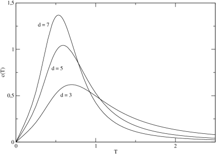
Figure 5: (a) Entropy $S(T)$ and (b) specific heat $c(T)$ data versus temperature $T$ for the Temperley-Lieb Hamiltonians with $\Delta=1/2$ corresponding to the $sl(n+1|n)$ invariant network models with $n=1,2,3$ $(d=3,5,7)$.

If we impose $\pi$-twisted boundary conditions in imaginary time direction, i.e. if we define a pseudo-partition function by use of the super-trace, we find a vanishing free energy for all temperatures consistent with the low-temperature asymptotics with central charge $c=0$.

5 Conclusion

In this paper we derived the complete low-lying energy spectrum of the quantum spin chain related to the $sl(n+1|n)$ supersymmetric network of [16]. Our analysis consists of two major steps. First, we established a proper Temperley-Lieb equivalence of the quantum spin chain with periodic/twisted boundary conditions to a spin-1/2 $XXZ$ chain with anisotropy $\Delta=1/2$ and suitable boundary conditions. We presented a representation theoretical approach as a simple alternative to the evaluation of the scaling dimensions and multiplicities in [33, 34]. Second, the leading logarithmic corrections to the conformal spectrum were derived. Our results indicate that the models of [16] and [15] belong to different universality classes. The calculations are based on an asymptotic analysis of non-linear integral equations for the finite temperature and finite size properties of the Heisenberg spin chain. These equations are exact for arbitrary size. By these means, also the thermodynamical properties of the supersymmetric Hamiltonians of Temperley-Lieb type were computed for arbitrary temperature. The specific heat exhibits a linear low-temperature behaviour with a slope corresponding to the central charge in the $\pi$-twisted sector.

Appendix

In this appendix we give a short account of the derivation of the multiplicity formulas and a proof of the completeness of states. All formulae are to be understood as for the generic Temperley-Lieb representations in the limit of $\lambda=2\Delta\to 1$ avoiding the explicit analysis of reducible but indecomposable representations. We begin with the characterization of the space of pseudo-vacua $\Omega_{N}^{p}$ containing all states $\omega$ on a chain of length $N$ with periodic boundary conditions annihilated by all operators $b_{1}$,…,$b_{N}$. If we label the canonical basis states of the local spaces $V$ with $j=1,...,d\ (=2n+1)$ and define $U:V\to V$ by $U_{i,j}:=\delta_{i,d+1-j}$, the space $\Omega_{N}^{p}$ is mapped by $U\otimes{\rm id}\otimes U\otimes{\rm id}\otimes...$ onto a space of states that are annihilated by the application of dual states $\left<\psi\right|:=\sum_{j=1}^{d}\left<j,d+1-j\right|$ and $\left<\tilde{\psi}\right|:=\sum_{j=1}^{d}(-1)^{j+1}\left<j,d+1-j\right|$ on (odd,even)- and (even,odd)-indexed nearest-neighbours, respectively. We introduce a $q$-deformed version of this space by demanding annihilation by $\sum_{j=1}^{d}q^{j-(d+1)/2}\left<j,d+1-j\right|$ and $\sum_{j=1}^{d}(-1)^{j+1}q^{j-(d+1)/2}\left<j,d+1-j\right|$. The dimension of the space is independent of $q$ (see [35]) and can be easily enumerated in the limit $q\to\infty$. The condition for the states is simply that the sequence $(d,1)$ never occurs. The counting problem is now reduced to the evaluation of traces of powers of the $d\times d$ adjacency matrix $A$ with entries 1 everywhere except for one 0 at the position $(d,1)$. The only non-zero eigenvalues are $\alpha_{\pm}=(d\pm\sqrt{d^{2}-4})/2$, where $\alpha_{-}=1/\alpha_{+}$. Hence

$$d(N):={\rm Tr}A^{N}=\alpha_{+}^{N}+\alpha_{-}^{N},$$ (51)

which proves (36) for $N>0$. Defining the diagonal $d\times d$ matrix $R:={\rm diag}(+1,-1,+1,-1,..)$ we find

$${\rm Tr}(AR)^{N}=d^{e}(N)-d^{o}(N),$$ (52)

where $d^{e}(N)$ and $d^{o}(N)$ are the dimensions of the subspaces with even and odd numbers of fermions, respectively. The only non-zero eigenvalues of $AR$ are $(1\pm{\rm i}\sqrt{3})/2$, hence $d^{e}(N)-d^{o}(N)=2\cos\left(\frac{\pi}{3}N\right)$ proving (43). Finally, we like to count the number of states covered by the constructed representations. The dimension of each $k$-sector ($k=0,1,...,L/2$) is $L\choose k$ and appears $d(L-2k)$ times for $k<L/2$ and once for $k=L/2$. Hence the number of states is

$$\sum_{k=0}^{L/2-1}{L\choose k}\left(\alpha_{+}^{L-2k}+\alpha_{+}^{-(L-2k)}\right)+{L\choose L/2}=\sum_{k=0}^{L}{L\choose k}\alpha_{+}^{L-2k}=\alpha_{+}^{L}(1+\alpha_{+}^{-2})^{L}=d^{L}.$$ (53)

References

- [1] R. J. Baxter: Exactly Solved Models in Statistical Mechanics (London: Academic Press, 1982).
- [2] H. N. V. Temperley and E. Lieb: Proc. R. Soc. Lond. A 322 (1971) 251.
- [3] P. Martin: Potts Models and Related Problems in Statistical Mechanics (World Scientific, 1991)
- [4] H. A. Bethe, Z. Phys. 71 (1931) 205.
- [5] A. A. Belavin, A. M. Polyakov and A. B. Zamolodchikov, Nucl. Phys. B 241 (1984) 333.
- [6] J. L. Cardy: Phase Transitions and Critical Phenomena, Vol. 11, Editors C. Domb and J. L. Lebowitz (London: Academic Press, 1988).
- [7] A. V. Razumov and Yu. Stroganov: Spin chains and combinatorics, J. Phys. A: Math. Gen. 34 (2001) 3185.
- [8] A. V. Razumov and Yu. Stroganov: Combinatorial nature of ground state vector of loop model, Theor. Math. Phys. 138 (2004) 333-337.
- [9] A. V. Razumov and Yu. Stroganov: loop model with different boundary conditions and symmetry classes of alternating sign matrices, Theor. Math. Phys. 142 (2005) 237-243.
- [10] M. T. Batchelor, J. de Gier and B. Nienhuis: The quantum symmetric XXZ chain at Delta , alternating sign matrices and plane partitions, J. Phys. A: Math. Gen. 34 (2001) L265.
- [11] Greg Kuperberg: Another proof of the alternating sign matrix conjecture, Internat. Math. Res. Notices (1996) 139-150.
- [12] S. Eggert, I. Affleck and M. Takahashi, Phys. Rev. Lett. 73 (1994) 332.
- [13] J. Sirker and M. Bortz, J. Stat. Mech. P01007 (2006).
- [14] J. T. Chalker and P. D. Coddington, J. Phys. C 21 (1988) 2665.
- [15] R. Gade, J. Phys. A 31 (1998) 4909.
- [16] I. A. Gruzberg, A. W. W. Ludwig and N. Read, Phys. Rev. Lett. 82 (1999) 4524, cond-mat/9902063.
- [17] F. Essler, H. Frahm and H. Saleur: Continuum Limit of the Integrable Superspin Chain, Nucl. Phys. B 712 (2005) 513-572.
- [18] A. Altland and M. Zirnbauer, Phys. Rev. B 55 (1997) 1142.
- [19] R. J. Baxter, J. Stat. Phys. 28 (1982) 1.
- [20] K. Okamoto and K. Nomura, Phys. Lett. A 169 (1992) 433.
- [21] A. Klümper, Ann. Physik 1 (1992) 540, Z. Phys. B 91 (1993) 507.
- [22] T. Koma, Prog. Theor. Phys. 78 (1987) 1213, Prog. Theor. Phys. 81 (1989) 783.
- [23] M. Takahashi, Phys. Rev. B 43 (1991) 5788, Phys. Rev. B 44 (1991) 12382.
- [24] J. Suzuki, Y. Akutsu and M. Wadati, J. Phys. Soc. Japan 59 (1990) 2667-2680.
- [25] S. Lukyanov, Nucl. Phys. B 522 (1998) 533.
- [26] A. Klümper: Integrability of quantum chains: theory and applications to the spin-1/2 chain, in Quantum magnetism, Editors U. Schollwöck, J. Richter, D. J. J. Farnell and R. F. Bishop (Springer, Lecture Notes in Physics, Vol. 645, in press 2004).
- [27] A. Klümper: The spin-1/2 Heisenberg chain: thermodynamics, quantum criticality and spin-Peierls exponents, Euro. Phys. J. B 5 (1998) 677, cond-mat/9803225.
- [28] A. Klümper and D. C. Johnston: Thermodynamics of the Spin Antiferromagnetic Uniform Heisenberg Chain, Phys. Rev. Lett. 84 (2000) 4701.
- [29] N. M. Bogoliubov, A. G. Izergin and V. E. Korepin, Nucl. Phys. B 275 (1986) 687.
- [30] N. M. Bogoliubov, A. G. Izergin and N. Y. Reshetikin, J. Phys. A 20 (1987) 5361.
- [31] N. M. Bogoliubov, A. G. Izergin and V. E. Korepin: Quantum Inverse Scattering Method and Correlation Functions (Cambridge: Cambridge University Press, 1993).
- [32] A. Klümper, T. Wehner and J. Zittartz: Conformal spectrum of the six-vertex model, J. Phys. A 26 (1993) 2815-2827.
- [33] N. Read and H. Saleur, Nucl. Phys. B 613 409 (2001), hep-th/0106124.
- [34] J.-F. Richard and J. L. Jacobsen: Eigenvalue amplitudes of the Potts model on a torus, Nucl. Phys. B 769 (2007) 256-274.
- [35] B. Aufgebauer and A. Klümper: Quantum spin chains of Temperley-Lieb type: periodic boundary conditions, spectral multiplicities and finite temperature, J. Stat. Mech. P05018 (2010), arXiv:1003.1932.