The energy density in the planar Ising model
Abstract.
We study the critical Ising model on the square lattice in bounded simply connected domains with and free boundary conditions. We relate the energy density of the model to a discrete fermionic spinor and compute its scaling limit by discrete complex analysis methods. As a consequence, we obtain a simple exact formula for the scaling limit of the energy field one-point function in terms of the hyperbolic metric. This confirms the predictions originating in physics, but also provides a higher precision.
Key words and phrases:
Ising model, energy density, discrete analytic function, fermion, spinor, conformal invariance, hyperbolic geometry, conformal field theory1. Introduction
1.1. The model
The Lenz-Ising model in two dimensions is probably one of the most studied models for an order-disorder phase transition, exhibiting a very rich and interesting behavior, yet well understood both from the mathematical and physical viewpoints [Bax89, McWu73, Pal07].
After Kramers and Wannier [KrWa41] derived the value of the critical temperature and Onsager [Ons44] analyzed the behavior of the partition function for the Ising model on the two-dimensional square lattice, a number of exact derivations were obtained by a variety of methods. Thus it is often said that the 2D Ising model is exactly solvable or integrable. Moreover, it has a conformally invariant scaling limit at criticality, which allows to use Conformal Field Theory (CFT) or Schramm’s SLE techniques. CFT provides predictions for quantities like the correlation functions of the spin or the energy fields, which in principle can then be related to SLE.
In this paper, we obtain a rigorous, exact derivation of the one-point function of the energy density, matching the CFT predictions [DMS97, Car84, BuGu93]. We exploit the integrable structure of the 2D Ising model, but in a different way from the one employed in the classical literature. Our approach is rather similar to Kenyon’s approach to the dimer model [Ken00].
We write the energy density in terms of discrete fermionic spinors introduced in [Smi06]. These spinors solve a discrete version of a Riemann boundary value problem, which identifies them uniquely. In principle, this could be used to give an exact, albeit very complicated, formula, that one could try to simplify – a strategy similar to most of the earlier approaches. Instead we pass to the scaling limit, showing that the solution to the discrete boundary value problem approximates well its continuous counterpart, which can be easily written using conformal maps. Thus we obtain a short expression, approximating the energy density to the first order. Moreover, our method works in any simply connected planar domain, and the answer is, as expected, conformally covariant.
Similar spinors appeared in Kadanoff and Ceva [KaCe71] and in Mercat [Mer01], but their scaling limits with boundary conditions were not discussed before [Smi06].
Recall that the Ising model on a graph is defined by a Gibbs probability measure on configurations of (or up/down) spins located at the vertices: it is a random assignment of spins to the vertices of and the probability of a state is proportional to its Boltzmann weight , where is the inverse temperature of the model and is the Hamiltonian, or energy, of the state . In the Ising model with no external magnetic field, we have , where the sum is over all the pairs of adjacent vertices of .
1.2. The energy density
Let be a Jordan domain and let be a discretization of it by a subgraph of the square grid of mesh size . We consider the Ising model on the graph at the critical inverse temperature ; on the boundary of , we may impose the value to the spins or let them free (we call these and free boundary conditions respectively). Our main result about the energy density is the following:
Theorem.
Let and for each , let be the closest edge to in . Then, as , we have
where the subscripts and free denote the boundary conditions and is the element of the hyperbolic metric of .
A precise version of this theorem in terms of the energy density field is given in Section 1.4. This result has been predicted for a long time by CFT methods (see [DMS97, BuGu93] for instance), notably using Cardy’s celebrated mirror image technique [Car84]. However, CFT does not allow to determine the lattice-specific constant appearing in front of the hyperbolic metric element.
This is one of the first results where full conformal invariance (i.e. not only Möbius invariance) of a correlation function for the Ising model is actually shown. The proof does not appeal to the SLE machinery, although the fermionic spinor that we use is very similar to the one employed to prove convergence of Ising interfaces to SLE [ChSm09]. A generalization of our result with mixed boundary conditions could also be used to deduce convergence to SLE.
In the case of the full plane, the energy density correlations have been studied by Boutillier and De Tilière, using dimer model techniques [BoDT08, BoDT09]. However, their approach works in the infinite-volume limit or in periodic domains and does not directly apply to arbitrary bounded domains.
In the case of the half-plane, the energy density one-point function has been recently obtained by Assis and McCoy [AsMc11], using transfer matrix techniques.
The strategy for the proof of our theorem relies mainly on:
-
•
The introduction of a discrete fermionic spinor, which is a complex deformation of a certain partition function, and of an infinite-volume version of this spinor.
-
•
The expression of the energy density in terms of discrete fermionic spinors.
-
•
The proof of the convergence of the discrete spinors to continuous fermionic spinors, which are holomorphic functions.
1.3. Graph notation
Let us first give some general graph notation. Let be a graph embedded in the complex plane .
-
•
We denote by the set of the vertices of , by the set of its (unoriented) edges, by the set of its oriented edges.
-
•
We identify the vertices with the corresponding points in the complex plane (since is embedded). An oriented edge is identified with the difference of the final vertex minus the initial one.
-
•
Two vertices are said to be adjacent if they are the endpoints of an edge, denoted , and two distinct edges are said to be incident if they share an endvertex.
1.3.1. Discrete domains
-
•
We denote by the square grid of mesh size . Its vertices and edges are defined by
-
•
In order to keep the notation as simple as possible, we will only look at finite induced subgraphs of (two vertices of are linked by an edge in whenever they are linked in ), that we will also call discrete domains.
-
•
For a discrete domain , we denote by the dual graph of : its vertices are the centers of the bounded faces of and two vertices of are linked by an edge of if the corresponding faces of share an edge.
-
•
We denote by the set of vertices of that are at distance from a vertex of (i.e. that are adjacent in to a vertex of ) and by the set of edges between a vertex of and a vertex of . The vertices in appear with multiplicity: if a vertex of is at distance to several vertices of , then it appears as as many distinct elements of . In other words, there is a one-to-one correspondence between and .
-
•
We denote by the centers of the faces of that are adjacent to a face of . We denote by the set of dual edges between a vertex of and a vertex of . For an edge we denote by its dual ( and intersect at their midpoint).
-
•
We write for and for .
-
•
We denote by the set of horizontal (i.e. parallel to the real axis) edges of and by the set of the vertical ones.
-
•
We denote by and the medial graph of : its vertices are the midpoints of the edges of and the medial edges link midpoints of incident edges of .
-
•
We say that a family of discrete domains (with for each ) approximates or discretizes a continuous domain if for each , is the largest connected induced subgraph of contained in .
1.3.2. Ising model with boundary conditions
The Ising model (with free boundary condition) on a finite graph (in this paper, will be a discrete domain or its dual ) at inverse temperature is a model whose state space is given by : a state assigns to every vertex of a spin . The probability of a configuration is
with the energy (or Hamiltonian) of a configuration given by
and the partition function by
Given a graph with boundary vertices (like with ) the Ising model on with boundary condition is defined as the Ising model on , with extra spins located at the vertices of that are set to and with energy
where is the set of edges linking vertices of .
In this paper, we will be interested in the Ising model with free and boundary conditions on discrete square grid domains at the critical inverse temperature , when the mesh size is small.
We will from now on omit the inverse temperature parameter in the notation and will denote by and the probability measures of the Ising model on at with free and boundary conditions and by and the corresponding expectations.
1.4. The energy density
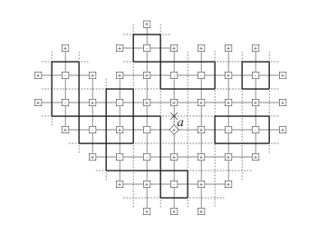
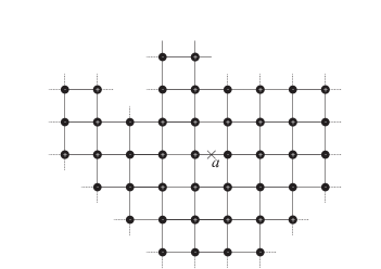
Let be a discrete domain and let be the midpoint of a horizontal edge of . We introduce the two quantities and , called average energy density (with free and boundary conditions), defined by
where and are respectively the (horizontal) edge and the dual (vertical) edge, the midpoint of both of which is (see Figures 1.1 and 1.2). The quantity is the infinite-volume limit of the product of two adjacent spins (it can be found in [McWu73], Chapter VIII, Formula 4.12, for instance). The energy density field is the fluctuation of the product of adjacent spins around this limit: it measures the distribution of the energy among the edges, as a function of their locations. We are considering horizontal edges on and vertical edges on for concreteness and for making the notation simpler, but our results are rotationally invariant.
We can now state the main result of this paper, which is the conformal covariance of the average energy density:
Theorem 1.
Let be a simply connected domain and let . Consider a family of discrete domains approximating and for each , let be the midpoint of horizontal edge that is the closest to . Then as , uniformly on the compact subsets of , we have
being the hyperbolic metric element of at . Namely, , where is the conformal mapping from to the unit disk such that 0 and .
The proof will be given in Section 1.6
Corollary 2.
The conclusions of Theorem 1 hold under the assumption that is a Jordan domain.
Proof.
We have that and are monotone respectively non-increasing and non-decreasing with respect to the discrete domain , as follows easily from the FKG inequality applied to the FK representation of the model (see [Gri06] Chapters 1 and 2, for instance): if , we have
If is a Jordan domain, we can approximate by monotone increasing and decreasing sequences of smooth domains, for which Theorem 1 applies, and deduce the result for . ∎
The central idea for proving Theorem 1 is to introduce a discrete fermionic spinor which is a two-point function ; it is defined in the next subsection. We then relate to the average energy density and prove its convergence to a holomorphic function .
1.5. Contour statistics and discrete fermionic spinor
1.5.1. Contour statistics
Let be a discrete domain. We denote by the set of edge collections such that every vertex belongs to an even number of edges of : in other words, by Euler’s theorem for walks, the edge collections are the ones that consist of edges forming (not necessarily simple) closed contours. For an edge , we denote by the set of configurations that do not contain and by the set of configurations that do contain .
Set . For a collection of edges , we denote by its cardinality. For we define
We now have the following representation of the energy density in terms of contour statistics.
Proposition 3.
Let be a horizontal edge and let its midpoint be . Then we have
Proof.
From the low-temperature expansion of the Ising model (see [Pal07], Chapter 1, for instance), there is a natural bijection between the configurations of spins on with boundary condition on and the edges collections : one puts an edge in the edge collection if the spins of at the endpoints of the dual edge are different. It is easy to see that the probability measure on induced by this bijection gives to each edge collection a weight proportional to , hence to , where as above (since ). The event that the spins at two adjacent dual vertices are the same (respectively are different) corresponds through the natural bijection to (respectively ), where is such that . Using that , we deduce the first identity.
From the so-called high-temperature expansion (see [Pal07], Chapter 1) we have that for the Ising model on with free boundary condition, the correlation of two spins is equal to
where is the set of edge collections such that every vertex in belongs to an even number of edges of and such that both belong to an odd number of edges of . At , we have (the fact that actually characterizes ).
Let us now take adjacent, set , and denote by and the sets of such that and respectively. From each , we can remove and obtain an edge collection in (this map is bijective) and to each , we can add and obtain an edge collection in . Hence we have
Using the relation , we obtain the second identity. ∎
1.5.2. Discrete fermionic spinor in bounded domain
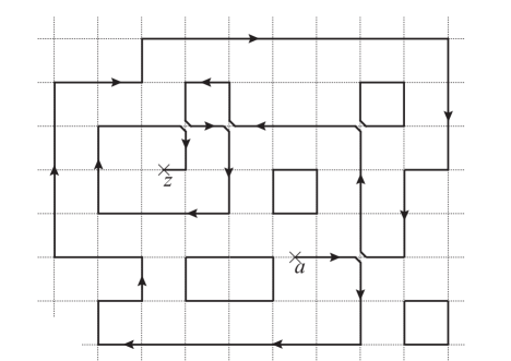
If is the midpoint of a horizontal edge and is the midpoint of an arbitrary edge , we denote by the set of consisting of edges of and of two half-edges (half of an edge between its midpoint and one of its ends) such that
-
•
one of the half-edges has endpoints ;
-
•
the other half-edge is incident to ;
-
•
every vertex belongs to an even number of edges or half-edges of .
For a configuration , we call admissible walk along , a sequence , such that
-
•
is the half-edge incident to ;
-
•
is the half-edge incident to ;
-
•
are edges;
-
•
and are incident for each ;
-
•
each edge appears at most once in the walk;
-
•
when one follows the walk and arrives at a vertex that belongs to four edges or half-edges of (we call this an ambiguity), one either turns left or right (going straight in that case is forbidden).
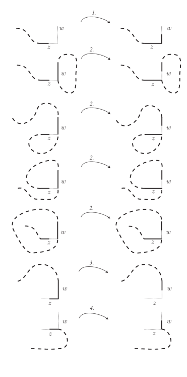
It is easy to see that, for any , such a walk always exists, though in general it is not unique (see Figure 1.3).
Given a configuration and an admissible walk along , we define the winding number of , denoted , by
where and are respectively the numbers of left turns and right turns that the admissible walk makes from to : it is the total rotation of the walk between and , measured in radians. More generally, we define the winding number of a rectifiable curve as its total rotation from its initial point to its final point, measured in radians. The following lemma shows that the winding number (modulo ) of a configuration is actually independent of the choice of the walk on .
Lemma 4.
For any , the winding number is independent of the choice of an admissible walk along .
The proof is given in Appendix A.
Thanks to Lemma 4, we can now define the discrete fermionic spinor that will be instrumental in our studies of the energy density.
Definition 5.
For any midpoint of a horizontal edge , we define the discrete fermionic spinor by
where denotes the number of edges and half-edges of , with the half-edges contributing each.
In this way, is a function, whose value at gives (up to an additive constant) the average energy density at . As we will see, moving the point accross the domain will allow to gain information about the effect of the geometry of the domain on the energy density.
1.5.3. Discrete fermionic spinor in the full plane
As mentioned above, the appearing in the definition of the average energy density (Section 1.4) is the infinite volume limit (or full-plane) average product of two adjacent spins, which one has to subtract in order for the effect of the shape of the domain to be studied. We now introduce a full-plane version of the discrete fermionic spinor, whose definition a priori seems quite different from the bounded domain version. It will allow to represent the energy density (with the correct additive constant) in terms of the difference of two discrete fermionic spinors.
Definition 6.
For with and being the midpoint of an horizontal edge, define by
where is the dimer coupling function of Kenyon (see [Ken00]), defined by
We set .
From our definitions up to now and from Proposition 3, we deduce the following:
Lemma 7.
Let be a discrete domain and be the midpoint of a horizontal edge of . Then the average energy density can be represented as
1.6. Convergence results and proof of Theorem 1
The core of this paper is the convergence of the discrete fermionic spinors to continuous ones, which are holomorphic functions. Let us define these functions first: for with , we define
where is the unique conformal mapping from to the unit disk with and (this mapping exists by the Riemann mapping theorem). Note that and both have a simple pole of residue at and that hence extends holomorphically to .
We can now state the key theorem of this paper:
Theorem 8.
For each , identify with the closest midpoint of a horizontal edge of and with the closest midpoint of an edge of . Then we have the following convergence results
where the convergence of is uniform on the compact subsets of away from the diagonal , the convergence of is uniform on away from the diagonal and the convergence of is uniform on the compact subsets of .
From this result, the proof of the main theorem follows readily: since we have (Lemma 7)
and since converges to , it suffices to check that
which follows readily by verifying that
To prove this, notice that since
by squaring this expression, it suffices to check that the residue of at vanishes. By contour integrating on a small circle around and using change of variable formula (since is conformal), we have
1.7. Proof of convergence
The rest of this paper is devoted to the proof of the key theorem (Theorem 8). This proof consists mainly of two parts:
-
•
The analysis of the discrete fermionic spinors and as functions of their second variable (Section 2):
- –
- –
-
–
We observe that has some specific boundary values on (Proposition 18).
-
•
The proof of convergence of functions , , (Section 3):
-
–
The convergence of follows directly from the convergence result of Kenyon for the dimer coupling function (Theorem 25).
-
–
We show that the family of functions is precompact on the compact subsets of : it admits convergent subsequential limits as (Proposition 26). Hence is also precompact on the compact subsets of away from the diagonal.
- –
-
–
Acknowledgements
This research was supported by the Swiss N.S.F., the European Research Council AG CONFRA, by EU RTN CODY, by the Chebyshev Laboratory (Department of Mathematics and Mechanics, St.-Petersburg State University) under RF governement grant 11.G34.31.0026 and by the National Science Foundation under grant DMS-1106588.
The authors would like to thank D. Chelkak for advice and useful remarks, as well as V. Beffara, Y. Velenik, K. Kytölä, K. Izyurov, C. Boutillier, B. de Tilière, for useful discussions. The first author would like to thank W. Werner for his invitation to Ecole normale supérieure, during which part of this work was completed.
2. Analysis of the Discrete Fermionic Spinors
In this section, we study the properties of the discrete fermionic spinors and that follow from their constructions. In the next section, we will use these properties to prove Theorem 8.
We study both spinors as functions and of their second variable, keeping fixed the medial vertex (which is the midpoint of a horizontal edge of ).
Let us first introduce the discrete versions of the differential operators and that will be useful in this paper: for a -valued function , we define, wherever it makes sense (i.e. for vertices of ),
In the case where one has that a vertex belongs to in the definition of , the boundary vertex is the one identified with the edge .
If is an oriented edge with and is a function we denote by the discrete partial derivative defined by .
2.1. Discrete holomorphicity
It turns out that the functions and are discrete holomorphic in a specific sense, which we call s-holomorphicity or spin-holomorphicity.
Let us first define this notion. With any medial edge , we associate a line of the complex plane defined by
where is the closest vertex to and is the closest dual vertex to . On the square lattice, the four possible lines that we obtain are and . When is a line in the complex plane passing through the origin, let us denote by the orthogonal projection on , defined by
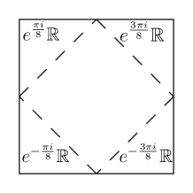
Definition 9.
Let be a collection of medial vertices. We say that is s-holomorphic on if for any two medial vertices that are adjacent in ,
where .
Remark 10.
Our definition is the same as the one introduced in [Smi10], except that the lines that we consider are rotated by a phase of , and that our lattice is rotated by an angle of , compared to the definitions there. In [ChSm09] this definition is also used, in the more general context of isoradial graphs.
Remark 11.
The definition of s-holomorphicity implies that a discrete version of the Cauchy-Riemann equations is satisfied: if is s-holomorphic and is such that the four medial vertices are in , then we have:
This can be found in [Smi10] (it follows by taking a linear combination of the four s-holomorphicity relations between the values ), as well as the fact that satisfying this difference equation is strictly weaker than being s-holomorphic.
Remark 12.
If is a simple counterclockwise-oriented closed discrete contour of medial edges and is the collection of points in surrounded by , then it is easy to check that for any function , we have
In particular this sum vanishes if is discrete holomorphic.
Proposition 13.
The function is s-holomorphic on .
Proof.
Let be two adjacent medial vertices and let be the medial edge linking them. Suppose that is the midpoint of a horizontal edge and that is the midpoint of a vertical edge. We prove the result in the case where (the other ones are symmetric). Denote by the half-edge between and and by the half-edge between and . For any , define as the symmetric difference of with : if is not in , add it, otherwise remove it, and similarly for . Clearly, is an involution mapping to and vice versa. Moreover, for , we have
| (2.1) |
This identity follows from considering the four possible cases, as shown in Figure 2.2:
-
(1)
If and , then we have , and .
-
(2)
If and , we have , and : there are a number of subcases, as shown in Figure 2.2, for which these relations are satisfied.
-
(3)
If and , we have , and : in this case, we can always choose an admissible walk on that is like in Figure 2.2.
-
(4)
If and , we have , and .
In all the four cases, it is then straightforward to check that equation 2.1 is satisfied. By definition of (Section 5), we finally deduce
which is the s-holomorphicity equation. ∎
The full-plane discrete spinor is also s-holomorphic:
Proposition 14.
The function is s-holomorphic on .
2.2. Singularity
Near the medial vertex , the functions and are not s-holomorphic: they both have a discrete singularity, but of the same nature, and consequently the difference is s-holomorphic on , including the point . Rather than defining the notion of discrete singularity, let us simply describe the relations that these functions satisfy near . For , let us denote by the medial vertex adjacent to , by the medial edge between and and by the line (as in Definition 9). Let be the horizontal edge with midpoint . Recall that is defined as (see Definition 5).
Proposition 15.
Near , the function satisfies the relations
Proof.
The first two relations are the s-holomorphicity relations and they are obtained in exactly the same way as the s-holomorphicity relations away from . Indeed, let us take the same notation as in the proof of Proposition 13 and consider the involutions , and defined by and respectively: as in the proof of Proposition 15, we have that these involutions preserve the projections on and respectively (a configuration is interpreted as a configuration of winding ).
For the last two relations, we have that the involutions and , respectively defined by and , are such that for any , we have
where is interpreted as a configuration with a path from to that makes a loop, of winding number . This follows from the same considerations as in the proof of Proposition 13. Hence, since , we obtain, by summing the above equations over all , the last two identities of Proposition 15. ∎
The function has the same type of discrete singularity as :
Proposition 16.
Near , the function satisfies exactly the same projection relations as the ones satisfied by the function , given by Proposition 15.
Proof.
See Appendix B, Proposition 33. ∎
Proposition 17.
The function is s-holomorphic on .
2.3. Boundary values
A crucial piece of information to understand the effect of the geometry of the discrete domain on the average energy density at is the boundary behavior of . On the set of boundary medial vertices , which link a vertex of and a vertex of , the argument of is determined modulo . For each , with being the midpoint of an edge between a vertex and a vertex , denote by the oriented outward-pointing edge at , identified with the number : it is a discrete analogue of the outward-pointing normal to the domain.
Proposition 18.
On , the argument of the value of is determined (modulo ): for each , we have
Proof.
From topological considerations, we have that if and , then : the winding number of any admissible walk from to is determined modulo (see Figure 2.3) and it is easy to check that is a real multiple of . Hence, the result follows from the definition of . ∎
2.4. Discrete integration
An essential tool that we will use for deriving the convergence of is the possibility to define a discrete version of the antiderivative of the square of an s-holomorphic function, cf. [Smi10].
Proposition 20.
Let be an s-holomorphic function on a discrete domain and let (where and ). Then there exists a (possibly multivalued) discrete analogue of the antiderivative
uniquely defined by and
where is the medial edge which is between and . If is simply connected, then the function is globally well-defined (single-valued). When the choice of the point is irrelevant, we will ommit it and simply write .
Remark 21.
It follows from the definition of that for any pair of adjacent vertices , we have
and similarly if are adjacent dual vertices. From there it is easy to see that if the mesh size is small, is a good approximation of .
We denote by and the restrictions of to and respectively. We have the following:
Proposition 22.
The function is discrete subharmonic and the function is discrete superharmonic: we have
If , then we have
where is the oriented edge from to , the midpoint of which is .
Proof.
For the subharmonicity/superharmonicity deduced from the s-holomorphicity of , see Lemma 3.8 in [Smi10] (the fact that the phases are different does not affect the result). The normal derivative statement follows directly from the definition of . ∎
In the case of the discrete fermionic spinor , the boundary condition for becomes particularly simple.
Proposition 23.
The function is constant on and for each ,
Proof.
The first statement follows from the construction of and from the boundary condition for (Proposition 18).
Remark 24.
Note that is single-valued (as follows from Proposition 23) and well-defined on but that the presence of a singularity near implies that and and are (at least a priori) not subharmonic or superharmonic near (more precisely at ).
3. Convergence of the Discrete Fermionic Spinors
We now turn to the convergence of the three functions as (Theorem 8). For this, we use the discrete results derived in the previous section: the s-holomorphicity, the discrete singularity and the boundary values. As we will discuss convergence questions, we will always, when necessary, identify the points of the complex plane with the closest vertices on the graphs considered. In this way, we will extend functions defined on the vertices of the graphs to functions defined on . In particular, for the discrete holomorphic spinors, when we write or for , we identify with the closest midpoint of a horizontal edge of and with the closest midpoint of an arbitrary edge of .
The convergence of almost immediately follows from the work of Kenyon [Ken00]:
Theorem 25.
For any . we have
uniformly on , where
Proof.
See the last paragraph of Appendix B. ∎
For the convergence of and , we proceed in two steps: we first show that the family of functions is precompact. Precompactness for will then readily follow from Theorem 25. We then identify uniquely the subsequential limits of ; this also identifies the ones of .
3.1. Precompactness
We now state our main precompactness result:
Proposition 26.
The family of functions
is precompact in the topology of uniform convergence on the compact subsets of , and hence the family of functions
is precompact in the topology of uniform convergence on the compact subsets of that are away from the diagonal.
Proof.
Set . By Proposition 18, we have that for any ,
By Theorem 25 and the fact that is smooth (and hence the number of medial vertices in is we deduce that the family of functions
is uniformly bounded and equicontinuous on the compact subsets of (since is uniformly convergent by Theorem 25). By Proposition 27 below, we obtain that the family of functions
is uniformly bounded and equicontinuous and hence we get the desired result by extending the functions in a uniformly continuous way to (for instance by piecewise-linear interpolation) and by using then Arzelà-Ascoli theorem.∎
Proposition 27.
There exists a universal constant such that for each and any s-holomorphic function , we have, for any ,
where .
Proof.
Consider the function , normalized to be at an arbitrary point. By subharmonicity (Proposition 22), a discrete integration by parts, and again by Proposition 22, we obtain
and from the last identity we also deduce that
On the other hand, from the construction of , it is easy to see that
By subharmonicity of , superharmonicity of and the construction of (Proposition 20), we have
By Theorem 3.12 in [ChSm09] (the construction there is the same as the one of our paper, up to a multiplication by an overall complex factor, which does not affect the result), there exists then a universal constant such that for any
We therefore deduce the desired inequalities. ∎
3.2. Identification of the limit
We can now uniquely identify the subsequential limits of as (we will often make a slight of abuse of notation and simply denote the family of functions by ). Let us start with a characterization of the continuous fermionic spinor (defined in Section 1.6).
Lemma 28.
The function is the unique holomorphic function such that
is bounded near and such that
| (3.1) |
where denotes the outward-pointing normal to .
The boundary condition 3.1 is equivalent to the condition that the antiderivative is single-valued on , constant on and satisfies
where denotes the normal derivative of in the outward-pointing direction.
Proof.
It is straightforward to check from the definition (Section 1.6) that has a simple pole of order and residue at and satisfies the boundary condition 3.1.
Let be another function with the same pole and boundary condition. Then the function defined by extends holomorphically to and satisfies
The function defined by has constant real part on and hence is constant on , by the maximum principle and the Cauchy-Riemann equations. Hence .
For the second part of the statement, notice that the boundary condition 3.1 implies that is purely real on , and hence must be constant on (when going along the boundary, one integrates , where is the tangent to the boundary, which is orthogonal to the normal ); this implies that is single-valued on (since is simply connected) and that
Conversely, it is easy to check that if is constant on , then for any , we have . Moreover, for any , we have that implies , which is equivalent to . ∎
Let us also give a lemma which will be useful to connect the discrete spinors to the continuous ones:
Lemma 29.
We have the uniform bound
Proof.
We now pass to the identification of the subsequential limits of as :
Proposition 30.
Let be a sequence with such that , uniformly on the compact subsets of . Then , where is defined in Section 1.6.
Proof.
For each , set .
Let us first remark that is holomorphic on , as it satisfies Morera’s condition: the integral of on any contractible contour vanishes, since it can be approximated by a Riemann sum involving (for small), which vanishes identically as explained in Remark 12. Fix a point . By Lemma 28, to identify with , it suffices to check that , defined by , satisfies the conditions of the second part of that lemma.
Let be the discrete antiderivative , as defined in Proposition 20, and let and denote the restrictions of to and , which are discrete subharmonic and superharmonic respectively (away from ), by Proposition 22. By Proposition 23, the function is constant on ; denote by this value. Fix a smooth doubly connected domain such that and (one of the component of is and the other is a simple loop surrounding ). Let us write and , where
-
•
is discrete harmonic, with on ,
-
•
is discrete subharmonic, with on ,
-
•
is discrete harmonic, with on ,
-
•
is discrete superharmonic, with on .
Let us further decompose as , where
-
•
is discrete harmonic with on and on .
-
•
is discrete harmonic with on and on .
The situation is hence the following: for any and such that , from the construction of , the superharmonicity of and the subharmonicity of , we have
| (3.2) |
It follows easily from Remark 21 that as , we have that , uniformly on the compact subsets of (since ).
Let us now check that satisfies the conditions of Lemma 28. and are uniformly close to each other on (they are equal to and there, and these functions are uniformly close to each other near , as follows easily from the convergence of ). To control , we use the following lemma, which is proven at the end of the section.
Lemma 31.
As , uniformly on the compact subsets of .
Observe that is uniformly bounded. Suppose indeed that it would not be the case and (by extracting a subsequence) that (say). We would have , since is harmonic and bounded on (since it is equal to there). We also would have , for the same reasons. By Equation 3.2 and Lemma 31, it would imply that would blow up on , which would contradict the fact that it converges uniformly to on the compact subsets of .
We deduce that and are uniformly bounded on .
We have that and as , uniformly on the compact subsets of . From the discrete Beurling estimate (see [Kes87]) and the uniform boundedness of and near , we readily obtain
and we deduce that continuously extends to and is constant there.
To show that for all , we consider the harmonic conjugate : it is the unique function (defined on the universal cover of and normalized to be at an arbitrary interior point ) such that is holormophic. By the Cauchy-Riemann equations, we have
where is the tangential derivative on in counterclockwise direction and the condition becomes . This latter condition is equivalent to the one that is non-increasing when going counterclockwise along (the universal cover of) .
Let us now check that this condition is satisfied. Take as before and denote by its universal cover.
For each , let be the discrete harmonic conjugate of (lifted to ), defined by integrating the discrete Cauchy-Riemann equations
and with the normalization . By subharmonicity of , we have on and hence, since on ,
and we deduce by the discrete Cauchy-Riemann equations that is non-increasing when going along the universal cover of in counterclockwise direction.
On the compact subsets of , since the (normalized) discrete derivatives of converge uniformly (see Remark 3.2 in [ChSm08]) to the derivatives of , it is easy to check that also converges uniformly to . Since is non-increasing (when going along the universal cover of ), we have that is locally uniformly bounded (uniformly with respect to ) on the universal cover of (if it would blow up there as , it would also blow up on ), and hence it is bounded everywhere on the closure of .
From there, we deduce that is non-increasing on the (counterclockwise-oriented) universal cover of : if it would not be the case, using again the discrete Beurling estimate [Kes87], we would obtain a contradiction (in the limit) with the fact that is non-decreasing. ∎
Proof of Lemma 31.
For , let us write for the discrete harmonic function such that on (this is the discrete harmonic measure of ). By uniqueness of the solution to the discrete Dirichlet problem, we can write
As , we have that on the compact subsets of , uniformly with respect to (this follows directly from Proposition 2.11 in [ChSm08]). By the construction of and the boundary conditions (Propositions 18 and 23), we have
for any , where is the midpoint of the edge between and its neighbor in . Since
is uniformly bounded by Lemma 29, we readily deduce that uniformly on the compact subsets of . ∎
Appendix A
We give here the proof of Lemma 4: for a configuration , the winding (modulo ) of an admissible walk on (see Figure 1.3) is independent of the choice of that walk.
Proof of Lemma 4.
Without loss of generality, half-edges of emanate from and in the same direction, so the winding is a multiple of .
Add a curve from to , which emanates in opposite direction from and run slightly off the lattice, so that is transversal to when an intersection occurs (see Figure 3.1). Let be the number of intersections of with .
Take any admissible walk along . The rest of can be split into disjoint cycles. So, if is the number of intersections of with , then . Indeed, their difference comes from cycles, which are disjoint from and so intersect an even number of times (see Figure 3.1).
The concatenation of and (when oriented) forms a loop , which has several intersections (when and run transversally). At each of those, change the connection so that there is no intersection, but instead two turns – one left and one right. Each of rearrangements either adds or removes one loop, so after the procedure, splits into simple loops with (see Figure 3.2).
Each of the simple loops has winding or , so .
We conclude that, mod , and so is independent of its particular choice. ∎
Appendix B
We prove here some technical results concerning the discrete full-plane spinor, introduced in Section 1.5.3. Let us denote by the rescaled version of Kenyon’s coupling function (defined in [Ken00]).
Lemma 32.
Proof.
Set and for any vertex and any , set . By translation invariance, we have
where, on the right hand sides, the two values of are orthogonal: one is purely real and the other purely imaginary. Let be two adjacent medial vertices, with being the midpoint of a horizontal edge of and the midpoint of a vertical one, and let . Then, there are four possibilities for the line :
-
•
If , we have that and
-
•
If , we have that and
-
•
If , we have and
and similarly
-
•
If , we have that and
and similarly
This concludes the proof of the lemma. ∎
We now turn to the singularity of (Proposition 16):
Proposition 33.
Near the midpoint of a horizontal edge , for , set and by . Then the function satisfies the relations
Proof.
Set and and . Exact values of the coupling function that can be found in [Ken00] (see Figure 6 there)
Using these values and the definition of , a straightforward computation gives
If we compute the projections of these values on the lines associated with the medial edges , a straightforward computation gives
which is the desired result. ∎
Let us now recall the result of Kenyon concerning the convergence of the function
Theorem 34 (Theorem 11 in [Ken00]).
As , we have
From there, we can prove Theorem 25:
Proof of Theorem 25.
By rescaling the lattice of the theorem above, one readily deduces that
uniformly on the sets . The proof of the theorem follows then from the definition of .∎
References
- [AsMc11] M. Assis, B. M. McCoy, The energy density of an Ising half-plane lattice, J. Phys. A:Math. Theor. 44:095003, 2011.
- [Bax89] R. Baxter, Exactly solved models in statistical mechanics. Academic Press Inc. [Harcourt Brace Jovanovich Publishers], London, 1989.
- [BoDT09] C. Boutillier, B. de Tilière, The critical Z-invariant Ising model via dimers: locality property. Comm. Math. Phys, to appear. arXiv:0902.1882v1, 2009.
- [BoDT08] C. Boutillier, B. de Tilière, The critical Z-invariant Ising model via dimers: the periodic case. PTRF 147:379-413, 2010. arXiv:0812.3848v1.
- [BuGu93] T. Burkhardt, I. Guim, Conformal theory of the two-dimensional Ising model with homogeneous boundary conditions and with disordered boundary fields, Phys. Rev. B (1), 47:14306-14311, 1993.
- [Car84] J. Cardy, Conformal invariance and Surface Critical Behavior, Nucl. Phys. B 240:514-532, 1984.
- [ChSm08] D. Chelkak, S. Smirnov, Discrete complex analysis on isoradial graphs. Adv. in Math., to appear. arXiv:0810.2188v1.
- [ChSm09] D. Chelkak, S. Smirnov, Universality in the 2D Ising model and conformal invariance of fermionic observables. Inv. Math., to appear. arXiv:0910.2045v2, 2009.
- [CFL28] R. Courant, K. Friedrichs, H. Lewy. Uber die partiellen Differenzengleichungen der mathematischen Physik. Math. Ann., 100:32-74, 1928.
- [DMS97] P. Di Francesco, P. Mathieu, D. Sénéchal, Conformal Field Theory, Graduate texts in contemporary physics. Springer-Verlag New York, 1997.
- [Gri06] G. Grimmett, The Random-Cluster Model. Volume 333 of Grundlehren der Mathematischen Wissenschaften, Springer-Verlag, Berlin, 2006.
- [Isi25] E. Ising, Beitrag zur Theorie des Ferromagnetismus. Zeitschrift für Physik, 31:253-258, 1925.
- [KaCe71] L. Kadanoff, H. Ceva, Determination of an operator algebra for the two-dimensional Ising model. Phys. Rev. B (3), 3:3918-3939, 1971.
- [Kau49] B. Kaufman, Crystal statistics. II. Partition function evaluated by spinor analysis. Phys. Rev., II. Ser., 76:1232-1243, 1949.
- [KaOn49] B. Kaufman, L. Onsager, Crystal statistics. III. Short-range order in a binary Ising lattice. Phys. Rev., II. Ser., 76:1244-1252, 1949.
- [Ken00] R. Kenyon, Conformal invariance of domino tiling. Ann. Probab., 28:759-795, 2000.
- [Kes87] H. Kesten, Hitting probabilities of random walks on , Stochastic Process. Appl. 25:164-187, 1987.
- [KrWa41] H. A. Kramers and G. H. Wannnier. Statistics of the two-dimensional ferromagnet. I. Phys. Rev. (2), 60:252-262, 1941.
- [Len20] W. Lenz, Beitrag zum Verständnis der magnetischen Eigenschaften in festen Körpern. Phys. Zeitschr., 21:613-615, 1920.
- [Mer01] C. Mercat, Discrete Riemann surfaces and the Ising model. Comm. Math. Phys., 218:177-216, 2001.
- [McWu73] B. M. McCoy, and T. T. Wu, The two-dimensional Ising model. Harvard University Press, Cambridge, Massachusetts, 1973.
- [Ons44] L. Onsager, Crystal statistics. I. A two-dimensional model with an order-disorder transition, Phys. Rev. (2), 65:117-149, 1944.
- [Pal07] J. Palmer, Planar Ising correlations. Birkhäuser, 2007.
- [Smi06] S. Smirnov, Towards conformal invariance of 2D lattice models. Sanz-Solé, Marta (ed.) et al., Proceedings of the international congress of mathematicians (ICM), Madrid, Spain, August 22–30, 2006. Volume II: Invited lectures, 1421-1451. Zürich: European Mathematical Society (EMS), 2006.
- [Smi10] S. Smirnov, Conformal invariance in random cluster models. I. Holomorphic fermions in the Ising model. Ann. Math. 172(2), 2010.
- [Yan52] C. N. Yang, The spontaneous magnetization of a two-dimensional Ising model. Phys. Rev. (2), 85:808-816, 1952.