Interference and inequality in quantum decision theory

Abstract

The quantum decision theory is examined in its simplest form of two-condition two-choice setting. A set of inequalities to be satisfied by any quantum conditional probability describing the decision process is derived. Experimental data indicating the breakdown of classical explanations are critically examined with quantum theory using the full set of quantum phases.

1 Introduction

There has been growing recognition that the quantum probability, as an intriguing extension of classical probability, may find its application well beyond the microscopic realm of atoms and elementary particles. Among them, an interesting possibility of applying quantum description on psychological process has attracted much recent attentions. Several authors have noted [1, 2, 3] that the quantum interference among different paths of events leading to the same decision can account for the paradoxical experimental observation of the violation of sure-thing principle [4, 5], that has mystified psychologists for quite some time. The said paradox refers to the two-choice experiment under two preconditions, in which people make certain choice under the first condition and also make the identical choice under the second condition, but make the opposite choice under the situation where the precondition is supposed to be an unknown combination of the first and the second. This experimentally observed phenomenon is in direct contradiction with the fundamental assumption of the independence axiom in classical decision making theory [6], that is built upon the concept of classical (Bayesian) probability [7]. There is now a glimmer of hope that the quantum probability might provide a basis for a unifying theory of human cognition which has been long sought-after [2].

The key concept in the quantum decision theory is the interference among the probabilities of choices in different preconditions. This is a direct result of the central assumption of quantum decision theory that the preconditions and the choices are represented by vectors residing in a Hilbert space, and the unknown precondition is represented by linear superposition of known preconditions. The interference term has a form of geometric mean of probabilities under known conditions that are to be added to the classical arithmetic mean, thus representing possible alternate psychological mechanism to the standard theory. The amount of interference is controlled by the phase parameters that are inherent in Hilbert space vectors. Appearance of these phase parameters, which can be adjusted to explain experimental numbers, has been at the heart of the seeming success of the quantum explanation of the violation of sure thing principle. Unfortunately, a simple and easy-to-understand presentation of quantum decision theory based on a coherent framework seems to be still lacking. Moreover, a systematic analysis of experimental numbers based on a single framework has been missing. As it stands, therefore, it seems hard either to prove or disprove the effectiveness of quantum description of decision making process.

In this note, we reexamine the quantum analysis of decision making process in its simplest form, with the use of projection operator formalism, to clarify the essential elements of the theory, and identify the minimal number of phase parameters involved in the quantum description. We further derive a set of inequalities for conditional probabilities that involve only classically observable quantities, that have to be satisfied by any quantum description, thus are suitable to judge the utility of quantum approaches to decision theory. We illustrate the procedure to extract quantum phase parameters uniquely in systematic fashion, using the data obtained from previous psychological experiments. Hopefully, with accumulations of more experimental data, our approach will eventually enable the critical examination of quantum decision making theories.

2 Preliminaries

As a preliminary exercise, we start by examining a trivial, but usually neglected relation binding the quantum probabilities. Consider a two level system in the state $\left|\psi\right>=\psi_{0}\left|0\right>+\psi_{1}\left|1\right>.$ The probabilities of finding the system in the state $\left|0\right>$ and $\left|1\right>$ are given, respectively by $p_{0}=\left|\left<0|\psi\right>\right|^{2}=\psi_{0}^{*}\psi_{0}$ and $p_{1}=\left|\left<1|\psi\right>\right|^{2}=\psi_{1}^{*}\psi_{1}$, which places the constraint $\psi_{0}^{*}\psi_{0}+\psi_{1}^{*}\psi_{1}=1$ on quantum amplitudes $\psi_{j}$. We ask a question what the probability of finding the system in an intermediate state $\left|K\right>=\kappa_{0}\left|0\right>+\kappa_{1}\left|1\right>$ is. The proportion of the states $\left|0\right>$ and $\left|1\right>$ in $\left|K\right>$ are given by $q_{0}=\kappa_{0}^{*}\kappa_{0}$ and $q_{1}=\kappa_{1}^{*}\kappa_{1}$, respectively, with constraint $q_{0}+q_{1}=1$. The answer is immediately obtained as $p_{K}=\left|\left<K|\psi\right>\right|^{2}$ in the form

$$p_{K}=\frac{(2q_{0}p_{0})+(2q_{1}p_{1})}{2}+\sqrt{(2q_{0}p_{0})(2q_{1}p_{1})}\cos\theta,$$ (1)

where the relative quantum phase $\theta$ is defined through $\kappa_{0}^{*}\kappa_{1}\psi_{0}^{*}\psi_{1}=e^{i\theta}\sqrt{q_{0}q_{1}p_{0}p_{1}}$. The first term of (1) is the arithmetic mean of joint probabilities $q_{0}p_{0}$ and $q_{1}p_{1}$, as expected in usual classical intuition, while the second term, representing the quantum interference is given in the form of the geometric mean with the weight given by cosine of the quantum phase. With the obvious relation $-1\leq\cos\theta\leq 1$, we find

$$\left(\sqrt{q_{0}p_{0}}-\sqrt{q_{1}p_{1}}\right)^{2}\leq p_{K}\leq\left(\sqrt{q_{0}p_{0}}+\sqrt{q_{1}p_{1}}\right)^{2}.$$ (2)

3 Quantum conditional probabilities

Let us consider an agent facing a choice between two actions which we call $\left|0\right>$ and $\left|1\right>$. Let us further assume that his choice is conditional to an event that can take two outcome, $\left|0\right)$ and $\left|1\right)$, that precedes his choice. The quantum mechanical description of this agent is achieved by the state

$$\left|\left|\Psi\right)\right>=\left|0\right)\left|\!\right.\psi^{(0)}\left.\!\right>+\left|1\right)\left|\!\right.\psi^{(1)}\left.\!\right>,$$ (3)

with

$$\!\!\!\!\!\!\!\!\!\!\!\!\!\!\!\!\left|\!\right.\psi^{(0)}\left.\!\right>=\psi^{(0)}_{0}\left|0\right>+\psi^{(0)}_{1}\left|1\right>,$$

$$\!\!\!\!\!\!\!\!\!\!\!\!\!\!\!\!\left|\!\right.\psi^{(1)}\left.\!\right>=\psi^{(1)}_{0}\left|0\right>+\psi^{(1)}_{1}\left|1\right>,$$ (4)

where four $\psi^{(k)}_{j}$ are complex numbers. The conditional probability of agent taking action $\left|j\right>$ after observing the event $\left|k\right)$ is given by $p^{(k)}_{j}=|\psi^{(k)}_{j}|^{2}$. Naturally, $\psi^{(k)}_{j}$ are constrained by the normalization

$$\psi^{(k)*}_{0}\psi^{(k)}_{0}+\psi^{(k)*}_{1}\psi^{(k)}_{1}=1$$ (5)

for $k=0,1$. Let us now suppose that there is an intermediate event $\left|K\right)$ described by

$$\left|K\right)=\kappa^{(0)}\left|0\right)+\kappa^{(1)}\left|1\right),$$ (6)

with complex numbers $\kappa^{(k)}$ satisfying the constraint $\kappa^{(0)*}\kappa^{(0)}+\kappa^{(1)*}\kappa^{(1)}=1.$ For this intermediate event, the chance of the event $\left(k\right)$ occurring is given by $q^{(k)}=|\kappa^{(k)}|^{2}=\left(k|K\right)\left(K|k\right)$ .

Let us now consider the quantum state after the occurrence of the event $\left|K\right)$. This process can be thought of as a quantum measurement. Suppose a state $\left|\phi\right)$ is measured by an observer who finds the system in the state $\left|K\right)$. This process can be described by the application of non-unitary projection operator $\left|\phi\right>\to{\cal K}\left|\phi\right>$ with the definition

$${\cal K}=\frac{1}{\sqrt{\left<\left(\Psi|\right|K\right)\!\left(K|\!\left|\Psi\right)\right>}}\left|K\right)\!\left(K\right|.$$ (7)

When a partial measurement is made on the system in the state $\left|\left|\Psi\right)\right>$ of (3), it turns into

$$\left|\left|\Psi^{\prime}\right)\right>=\frac{1}{\sqrt{\left<\left(\Psi|\right|K\right)\!\left(K|\!\left|\Psi\right)\right>}}\left|K\right)\!\left(K|\!\left|\Psi\right)\right>$$ (8)

The partial matrix element $\left(K\right|\left.\!\!\left|\Psi\right)\right>$ is calculated as

$$\!\!\!\!\!\!\!\!\!\!\!\!\!\!\!\!\left(K\right|\left.\!\!\left|\Psi\right)\right>=\left<0\right|\!\left(K\right|\left.\!\!\left|\Psi\right)\right>\left|0\right>+\left<1\right|\!\left(K\right|\left.\!\!\left|\Psi\right)\right>\left|1\right>$$

$$\ \ =(\kappa^{(0)*}\psi^{(0)}_{0}+\kappa^{(1)*}\psi^{(1)}_{0})\left|0\right>+(\kappa^{(0)*}\psi^{(0)}_{1}+\kappa^{(1)*}\psi^{(1)}_{1})\left|1\right>.$$ (9)

In the state $\left|\left|\Psi^{\prime}\right)\right>$, the absolute value squared of the coefficient in front of the state $\left|K\right)\!\left|j\right>$ gives the probability of the agent’s action $\left<j\right>$ under the condition of the occurrence of the mixed event $\left|K\right)$, which we denote as $P^{K}_{j}$. We have

$$P^{K}_{j}=\frac{\left|{\left<j\right|\left(K\right|\left.\!\!\left|\Psi\right)\right>}\right|^{2}}{\left|{\left<0\right|\left(K\right|\left.\!\!\left|\Psi\right)\right>}\right|^{2}+\left|{\left<1\right|\left(K\right|\left.\!\!\left|\Psi\right)\right>}\right|^{2}},$$ (10)

which leads to the quantum description of the conditional probability $P^{K}_{j}$ in the form

$$P^{K}_{j}=\frac{q^{(0)}p^{(0)}_{j}+q^{(1)}p^{(1)}_{j}+2\sqrt{q^{(0)}q^{(1)}p^{(0)}_{j}p^{(1)}_{j}}\cos\theta_{j}}{1+2\sqrt{q^{(0)}q^{(1)}p^{(0)}_{0}p^{(1)}_{0}}\cos\theta_{0}+2\sqrt{q^{(0)}q^{(1)}p^{(0)}_{1}p^{(1)}_{1}}\cos\theta_{1}}.$$ (11)

Here, the phase $\theta_{j}$ is defined through

$$\kappa^{(0)}\kappa^{(1)*}\psi^{(0)*}_{j}\psi^{(1)}_{j}=e^{i\theta_{j}}\sqrt{q^{(0)}q^{(1)}p^{(0)}_{j}p^{(1)}_{j}}.$$ (12)

We clearly see that the quantum description has two extra phase parameters $\theta_{1}$ and $\theta_{2}$, on top of classical probabilities $q^{(k)}$ and $p^{(k)}_{j}$. These extra parameters might be thought of as representing internal psychological traits of the agents that admix the consideration of geometric average for intermediate event to the conventional arithmetic average. The $\theta$-dependent term in the enumerator represents the quantum interference of probabilities, while the ones in the denominator are the terms coming from “wave function renormalization” whose existence has been first noted in [3]. The general and explicit expressions of quantum conditional probability, (10) and (11) are the main result of the formal side of this work. The probability $P_{j}^{K}$ is reduced to the one given by the classical description

$$P_{j}^{K}[cl]=q^{(0)}p^{(0)}_{j}+q^{(1)}p^{(1)}_{j},$$ (13)

when these phase parameters have particular values $\theta_{1}=\theta_{2}=\pi$. It is obvious from (13), that, in classical description, the conditional probability $P^{K}_{j}$ necessarily falls between $p^{(0)}_{j}$ and $p^{(1)}_{j}$ because $q^{(0)}$ and $q^{(1)}$ are positive numbers adding up to the unity, namely

$$\min(p^{(0)}_{j},p^{(1)}_{j})\leq P^{K}_{j}\leq\max(p^{(0)}_{j},p^{(1)}_{j})\qquad({\rm Classical}).$$ (14)

This fact, that we should expect intermediate probability for intermediate event, is called sure-thing principle in psychological context. The necessity of the denominator in (11), for general value of phases, is related to the fact that the absolute values of two matrix elements $\left<0\right|\!\left(K\right|\left.\!\left|\Psi\right)\right>$ and $\left<1\right|\!\left(K\right|\left.\!\left|\Psi\right)\right>$ not summing up to one. This occurs because the conditional event $\left|K\right)$ alone does not exhaust the Hilbert space of preconditions, but has to be supplemented by the complementary state $\left|{\bar{K}}\right)$ defined as

$$\left|{\bar{K}}\right)=\kappa^{(1)*}\left|0\right)-\kappa^{(0)*}\left|1\right).$$ (15)

With this state, which is orthogonal to $\left|K\right)$, we have the completeness

$$\left|K\right)\left(K\right|+\left|{\bar{K}}\right)\left({\bar{K}}\right|=1,$$ (16)

and conditional probabilities $\left<j\right|\!\left(K\right|\left.\!\left|\Psi\right)\right>$ and $\left<j\right|\!\left({\bar{K}}\right.\left|\left|\Psi\right)\right>$, with $j=0,1$, do add up to unity.

We note that our treatment of intermediate precondition, (8), is essentially identical, in the language of quantum measurement theory, to the Lüders’ projection postulate [8] applied to a partial one-body measurement of a two-body system. If we consider repeated measurements with the same intermediate state $|K)$, it is reduced to the standard von Neumann’s projection postulate [9] with the pure state density matrix $\rho=|K)(K|$. If we further replace the pure state by a mixed state made up of states with incoherent random phases for $\kappa^{(0)}$ and $\kappa^{(1)}$, the interference effects cancel out among themselves [10]. The von Neumann postulate then yields the classical result, (13).

4 Quantum bound of conditional probability

Now, going back to the general expression (11), we consider the maximum and minimum for the quantum conditional probability. We first define the complementary value of $j$ as ${\bar{j}}=1-j$. Since the denominator is always positive, $\theta_{\bar{j}}=\pi$ will minimize it, and thus maximize $P^{K}_{j}$. We then have

$$P^{K}_{j} \!\!\!\!\!\!\!\!\!\!=\frac{q^{(0)}p^{(0)}_{j}+q^{(1)}p^{(1)}_{j}+2\sqrt{q^{(0)}q^{(1)}p^{(0)}_{j}p^{(1)}_{j}}\cos\theta_{j}}{1-2\sqrt{q^{(0)}q^{(1)}p^{(0)}_{\bar{j}}p^{(1)}_{\bar{j}}}+2\sqrt{q^{(0)}q^{(1)}p^{(0)}_{j}p^{(1)}_{j}}\cos\theta_{j}}$$ (17)

$$\!\!\!\!\!\!\!\!\!\!=1-\frac{\left(\sqrt{q^{(0)}p^{(0)}_{\bar{j}}}-\sqrt{q^{(1)}p^{(1)}_{\bar{j}}}\right)^{2}}{1-2\sqrt{q^{(0)}q^{(1)}p^{(0)}_{\bar{j}}p^{(1)}_{\bar{j}}}+2\sqrt{q^{(0)}q^{(1)}p^{(0)}_{j}p^{(1)}_{j}}\cos\theta_{j}}$$

which takes the maximum value with the choice $\theta_{j}=0$ Similarly, minimum value of $P_{j}^{K}$ is shown to be obtained at $\theta_{j}=\pi$ and $\theta_{\bar{j}}=0$. We have

$$\frac{\left(\sqrt{q^{(0)}p^{(0)}_{j}}-\sqrt{q^{(1)}p^{(1)}_{j}}\right)^{2}}{1-f_{j}}\leq P^{K}_{j}\leq\frac{\left(\sqrt{q^{(0)}p^{(0)}_{j}}+\sqrt{q^{(1)}p^{(1)}_{j}}\right)^{2}}{1+f_{j}}$$ (18)

where the correction term $f_{j}$ is give by

$$f_{j}=2\sqrt{q^{(0)}q^{(1)}}\left(\sqrt{p^{(0)}_{j}p^{(1)}_{j}}-\sqrt{p^{(0)}_{\bar{j}}p^{(1)}_{\bar{j}}}\right).$$ (19)

For the sake of arguments, let us for a moment limit ourselves to consider only those cases in which $f_{j}$ can be neglected. This occurs exactly when we have $p^{(0)}_{0}=p^{(1)}_{1}$ which also imply $p^{(0)}_{1}=p^{(1)}_{0}$ naturally. We then only need to look at the enumerators of (18) to identify the two bounds;

$$\frac{(2q^{(0)}p^{(0)}_{j})+(2q^{(1)}p^{(1)}_{j})}{2}\pm\sqrt{(2q^{(0)}p^{(0)}_{j})(2q^{(1)}p^{(1)}_{j})}.$$ (20)

We can now express the inequalities as quantum conditional probability of intermediate event is bounded by the sum and difference of weighted arithmetic and geometric means of probabilities of two events.

Going back to the general case, we consider the situation in which even the probability of the condition, $q^{(k)}$ is not known. We vary $q^{(0)}$ in (18) to maximize both bounds, and obtain

$$P^{K}_{j}(q_{max}^{(0)})=1,\quad P^{K}_{j}(q_{min}^{(0)})=0,$$ (21)

with

$$q_{max}^{(0)}=\frac{\left(\sqrt{p_{j}^{(0)}}-\sqrt{p_{j}^{(1)}}X_{j}\right)^{2}}{\left(\sqrt{p_{j}^{(0)}}-\sqrt{p_{j}^{(1)}}X_{j}\right)^{2}+\left(\sqrt{p_{j}^{(1)}}-\sqrt{p_{j}^{(0)}}X_{j}\right)^{2}}$$

$$q_{min}^{(0)}=\frac{\left(\sqrt{p_{j}^{(1)}}-\sqrt{p_{j}^{(0)}}X_{j}\right)^{2}}{\left(\sqrt{p_{j}^{(0)}}-\sqrt{p_{j}^{(1)}}X_{j}\right)^{2}+\left(\sqrt{p_{j}^{(1)}}-\sqrt{p_{j}^{(0)}}X_{j}\right)^{2}}$$ (22)

where

$$X_{j}=\sqrt{p_{j}^{(0)}p_{j}^{(1)}}-\sqrt{(1-p_{j}^{(0)})(1-p_{j}^{(1)})}.$$ (23)

We therefore obtain the quantum counterpart of sure-thing principle in the form of a trivial relation

$$0\leq P^{K}_{j}\leq 1\qquad({\rm Quantum}),$$ (24)

meaning that we should expect any value for conditional probability under unknown combination of preconditions. This is to be compared to the classical bound of sure-thing principle, (14).

5 Numerical examples

From practical point of view, in analyzing the results of psychological experiments, the main results of the previous section can be summarized as follows.

(i) Known unknown: When the probability of conditional event $q^{(k)}$ is known, the conditional probability for the event $K$, which is made up of probabilistically known combination of events $\left|0\right)$ and $\left|1\right)$, can take any value constrained by equation (18) with proper choice of two phase parameters $\theta_{1}$ and $\theta_{2}$.

(ii) Unknown unknown: When even the probability of conditional event $q^{(k)}$ is unknown, $P^{K}$, the conditional probability for the event $\left|K\right)$, can take any value between zero and one.

In order to scrutinize the predictive power of quantum decision theory, therefore, we need to have more than two experimental numbers for probability $P^{K}$ with different inputs $p^{(0)}_{j}$ and $p^{(1)}_{j}$, for a given “mind set” represented by a set $(\theta_{1},\theta_{2})$ and a known $q^{(0)}=1-q^{(1)}$. Conversely, any two sets of experimental numbers ($p^{(0)}_{j}$, $p^{(1)}_{j}$, $P^{K}_{j}$), which are within the bound of (18), can be fitted with some combination of values for $\theta_{1}$ and $\theta_{2}$. For a situation in which even the values of $q^{(0)}$ is unknown (but known to stay in a fixed value), the number of experimental data to be tested has to be more than three.

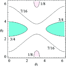
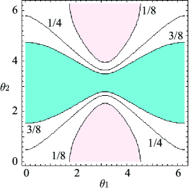
Figure 1: Contour graphs representing $P^{K}$ as a function of quantum phases $\theta_{1}$ and $\theta_{2}$. The white region represent the classical bound, inside of which the curve representing the classical prediction $P^{K}_{0}[cl]$ lies. The region with light shade (or pink) and with dark shade (or cyan) is where $P^{K}_{0}$ is below and above classical bound, respectively. The left side is the result of inputs $p^{(0)}=\frac{6}{8}$ and $p^{(1)}=\frac{1}{8}$, while the right side, of $p^{(0)}=\frac{3}{8}$ and $p^{(1)}=\frac{1}{8}$.

We first look at a fictitious two examples to get an idea how quantum theory works to provide numbers not attainable by classical probabilities. In Figure 1, we show contour graphs for $P^{K}=P^{K}_{0}$ as a function of $(\theta_{1},\theta_{2})$ with a given $(p^{(0)}_{0},p^{(1)}_{0})=(p^{(0)},p^{(1)})$ . We immediately notice the mirror symmetry along the axes $\theta_{1}=\pi$ and $\theta_{2}=\pi$, which is in fact evident from (10). The probability of condition is assumed to take $q^{(0)}=q^{(1)}=\frac{1}{2}$. In the graph in the left, we set $(p^{(0)},p^{(1)})$ $=(\frac{1}{8},\frac{6}{8})$, while in the graph in the right, it is $(p^{(0)},p^{(1)})$ $=(\frac{1}{8},\frac{3}{8})$. The white region is the value within classical bound of sure-thing principle, and the curved line in the white region represents the classical prediction $P^{K}[cl]$. The region with light shade (or pink) is where $P^{K}$ is below $\min(p^{(0)},p^{(1)})$ and the region with dark shade (or cyan) is where $P^{K}$ is above $\max(p^{(0)},p^{(1)})$. When $p^{(0)}$ and $p^{(1)}$ are closer, $P^{K}=0$ is more likely to get beyond classical sure-thing principle limit, as predicted by the quantum formula (10). In fact, for the case of fixed $q^{(0)}$, it is naturally not so much the violation of sure-thing principle, but the deviation form the classical value itself, that calls for the quantum explanation.

We now go on to examine the numbers from real world experiments performed up to now, which are summarized in Table 1. In these experiments, each participants is asked to choose from “bad’ or “good” behavior toward a fictitious opponent under certain condition on the knowledge of the choice of opponents (specified by $k$), and the percentages of people making “bad” and “good” choices are recorded as $p^{(k)}_{0}=p^{(k)}$ and $p^{(k)}_{1}=1-p^{(k)}$. Participants were told that they and their opponents were under prisoner’s dilemma-type situation, where one’s “bad” choice would be rewarded in the expense of his opponent, but he and his opponent would both benefit by both making “good” choice together, compared to both making “bad” choices. Experiments were done with real financial reward at stake. Experiments are done under three conditions. In one of them ($k=0$), they are told that the opponent have chosen the “bad” strategy, and in another ($k=1$), they are told that the other have gone “good”. In the third situation, they are told that the choice of the other is unknown ($K$), for which case, the probability of participants’ choosing “good” and “bad” behaviors are written as $P^{K}_{0}=P^{K}$ and $P^{K}_{1}=1-P^{K}$.

For all experiments, it is difficult to estimate the probabilities $q^{(k)}$, since this number is to represent “unknown” condition, not a testable quantity. Here, we simply assume, as a working hypothesis, that they are given by $q^{(0)}=q^{(1)}=\frac{1}{2}$. In all examples in Table 1, the numbers for $P^{K}$ are not only far from the classical prediction $P^{K}[cl]$ given by (13), but also are found to fall below $\min(p^{(0)},p^{(1)})$, which is the limit set by sure-thing principle. Namely, sure-thing principle is broken in all four experiments. It is also clear that they are well within the quantum bounds, (18) whose lower and upper bounds are written as $P^{K}_{min}$ and $P^{K}_{max}$ in the Table 1.

Authors / Year	$p^{(0)}$	$p^{(1)}$	$P^{K}_{exp}$	$P^{K}[cl]$	$P^{K}_{min}$	$P^{K}_{max}$
Shafir &Tversky / 1992 [4]	0.97	0.84	0.63	0.91	0.02	0.98
Croson / 1999 [11]	0.67	0.32	0.30	0.45	0.03	0.97
Li & Taplin / 2002 [12]	0.83	0.66	0.60	0.75	0.01	0.99
Busemeyer et al. / 2006 [13]	0.91	0.84	0.66	0.88	0.00	1.00

Table 1: Summary of experimental numbers of the conditional probabilities, $p^{X}=p^{X}_{0}=1-p^{X}_{1}$, representing the percentage of participants choosing “bad” move under different conditions signified by $X=(0),(1)$ and $K$. First three columns are the experimental data, the fourth, the classical prediction for $p^{K}$, and the last two, the quantum lower and upper bounds.

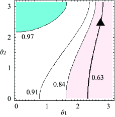
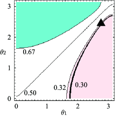
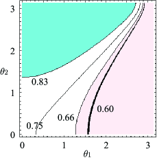
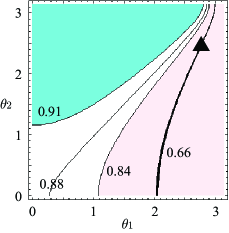
Figure 2: Contour graphs representing $P^{K}$ as a function of quantum phases $\theta_{1}$ and $\theta_{2}$. Values of $p^{(0)}$ and $p^{(1)}$ are taken from experiments found in Table 1. The white region represent the classical bound, inside of which the curve representing the classical prediction $P^{K}_{0}[cl]$ lies. The region with light shade (or pink) and with dark shade (or cyan) is where $P^{K}_{0}$ is below and above classical bound, respectively. The solid line is the trajectory of $(\theta_{1},\theta_{2})$ giving the experimental $P^{K}$. The triangles in three of the graphs points to the common value of $(\theta_{1},\theta_{2})$ where their solid lines cross each other.

In Figure 2, we show contour plot of $P^{K}$ as a function of two quantum phase angles $(\theta_{1},\theta_{2})$. As before, the white region is the value of $P^{K}$ within classical bound of sure-thing principle, and the curved line in the white region represents the classical prediction $P^{K}[cl]$. The regions with light shade (or pink) and dark shade (or cyan) are where $P^{K}$ is below or above the classical sure-thing principle limit, and solid line, falling within light-shaded (pink) region in all four examples, represents the set of phases $(\theta_{1},\theta_{2})$ that gives the experimentally observed $P^{K}$ values.

Broadly speaking, all graphs share similar appearance. But upon close examination by superimposing them, we observe the following two points:

(i) The result of Li and Taplin [12] is an “odd man out”, and the experimental solid line of the graph of Li and Taplin do not share any point with the lines from the other three experiments.

(ii) The results of Shafir and Tversky [4], Croson [11], and Busemeyer et. al. [13] give a consistent single choice of the phase $(\theta_{1},\theta_{2})\approx(0.27,0.25)$, marked by the solid triangle, at which point the experimental solid lines of three graphs cross each other.

A very optimistic interpretation is that in the three “consistent” experiments, groups of participants share common psychological traits that is indeed successfully described by quantum decision theory with a single set of quantum phases $(\theta_{1},\theta_{2})$. And in Li and Taplin experiment, the psychological makeup of the participants was markedly different from all other experiments. This experiment is presumably described by quantum theory with some other value of phases, which should lie somewhere on the solid line. A somberer view is that, we still lack both sufficient number and sufficient accuracy in the experimental data, and it is too early to call either success or the failure of quantum description of these psychological conditional probabilities.

In either way, through these numerical examples, we now have a clearer view on how to sort out the experimental numbers. With the accumulation of more experimental data, preferably with finer control of conditions, we may eventually hope to judge phenomenological applicability and predictive power of quantum decision theory.

6 Prospects

In this work, we have identified the minimal additional element of quantum theory viz à viz classical theory of conditional decision probability in two-by-two settings. It is straightforward to extend the treatment here to the case of more than two conditional events, and also to more than two choices for the agent. Suppose there are $M$ conditional events, to each of which there are $N$ choices. The number of relative phase appearing in the expression of conditional probability is the ${}_{N}C_{2}$, and there should be $M$ of these quantities. Thus the number of newly introduced parameters in the quantum description is $\frac{MN(N-1)}{2}$.

The success of quantum decision theory, if it is eventually obtained with more data, can mean one of two things. It can simply represent successful phenomenology with sufficient number of parameters and sufficient flexibility in formulation that can effectively simulate a more involved classical decision theory with sub-divided psychological conditions and cases. It can also mean a genuine quantum nature of some elements in psychological process in decision making. A parallel could be drawn from the quantum game theory [14, 15], which is shown to be applicable, on one hand, to non-quantum settings due to its effective inclusion of altruistic game strategy [16], and, on the other hand, is shown to include truly quantum effects that come from quantum interference [17]. To rigorously test the existence or the absence of genuinely quantum effect, we might need to consider decision making experiment with incomplete information, analogous to the Harsanyi type quantum game [18] in which breaking of the Bell inequality [19] can be directly tested.

Acknowledgments
This work has been partially supported by the Grant-in-Aid for Scientific Research of Ministry of Education, Culture, Sports, Science and Technology, Japan under the Grant Numbers 21540402 and 20700236.

References

- [1] D. Aerts, D. and S. Aerts, Applications of quantum statistics in psychological studies of decision processes, Found. Sci. 1 (1994) 8597.
- [2] E. M. Pothos and J. R. Busemeyer, A quantum probability explanation for violations of ’rational’ decision theory, Proc. Roy. Soc. B 276 (2009) 2171.
- [3] A. Yu. Khrennikov, E. Haven, Quantum mechanics and violations of the sure-thing principle: The use of probability interference and other concepts, J. Math. Psychol. 53 (2009) 378.
- [4] E. Shafir and A. Tversky, Thinking through uncertainty: nonconsequential reasoning and choice, Cogn. Psychol. 24 (1992) 449.
- [5] A. Tversky and E. Shafir, The disjunction effect in choice under uncertainty, Psychol. Sci. 3 (1992) 30509.
- [6] J. v.on Neumann, O. Morgenstern, “Theory of games and economic behavior”, (Princeton U. P., 1947).
- [7] L. J. Savage, “The foundation of statistics”, (Wiley, New York, 1954).
- [8] G. Lüders, Über die Zustandsänderung durch den Messprozess, Ann. Phys. (Leipzig) 8 (1951), 322.
- [9] J. von Neumann, ”Mathematical foundations of quantum mechanics”, (Princeton Univ. Press, Princeton, N.J., 1955).
- [10] N. Gisin, Quantum measurements and stochastic process, Phys. Rv. Lett. 52 (1984), 1657.
- [11] R. Croson, The disjunction effect and reason-based choice in games, Organ. Behav. Hum. Decis. Process. 180 (1999) 118.
- [12] S. Li and J. Taplin, Examining whether there is a disjunction effect in Prisoner’s Dilemma games, Chin. J. Psychol. 44 (2002) 25.
- [13] J. R. Busemeyer M. Matthew and Z. A. Wang, Quantum game theory explanation of disjunction effects, Proc. 28th Ann. Conf. Cogn. Sci. Soc. (eds. R. Sun and N. Miyake) (2006) 131.
- [14] D.A. Meyer, Quantum strategies, Phys. Rev. Lett. 82 (1999) 1052.
- [15] J. Eisert, M. Wilkens and M. Lewenstein, Quantum games and quantum strategies, Phys. Rev. Lett. 83 (1999) 3077.
- [16] T. Cheon, Altruistic duality in evolutionary game theory, Phys. Lett. A318 (2003) 327.
- [17] T. Cheon and I. Tsutsui, Classical and quantum contents of solvable game theory on Hilbert space, Phys. Lett. A348 (2006) 147.
- [18] T. Cheon and A. Iqbal, Bayesian Nash equilibria and Bell inequalities, Phys. Soc. Jpn. 77 (2008) 024801 (6p).
- [19] J. S. Bell, On the Einstein-Podolsky-Rosen paradox, Physics 1 (1964) 195.