Exceptional Points in a Microwave Billiard with
Time-Reversal Invariance Violation

Abstract

We report on the experimental study of an exceptional point (EP) in a dissipative microwave billiard with induced time-reversal invariance (${\mathcal{T}}$) violation. The associated two-state Hamiltonian is non-Hermitian and non-symmetric. It is determined experimentally on a narrow grid in a parameter plane around the EP. At the EP the size of ${\mathcal{T}}\,$violation is given by the relative phase of the eigenvector components. The eigenvectors are adiabatically transported around the EP, whereupon they gather geometric phases and in addition geometric amplitudes different from unity.

We present experimental studies of two nearly degenerate eigenmodes in a dissipative microwave cavity with induced ${\mathcal{T}}$violation. Due to the dissipative nature of the system the associated Hamiltonian is not Hermitian GW88 ; MF80 ; HH04 ; R08 and thus may possess an exceptional point (EP), where two or more eigenvalues and also the associated eigenvectors coalesce. In contrast, at a degeneracy of a Hermitian Hamiltonian, a so-called diabolical point (DP), the eigenvectors are linearly independent B84 ; BD03 . The occurrence of exceptional points Ka66 ; MF80 in the spectrum of a dissipative system was studied in quantum physics La95 as well as in classical physics EPTh09 . It has been demonstrated, that this is not only a mathematical but also a physical phenomenon. The first experimental evidence of EPs came from flat microwave cavities Phillip ; D01 ; Dembo2003 ; Metz , which are analogues of quantum billiards QB . Subsequently EPs were observed in coupled electronic circuits SHS04 and recently in chaotic microcavities and atom-cavity quantum composites Lee2009 . The present contribution is the first experimental study of an EP under ${\mathcal{T}}\,$violation. It is induced via magnetization of a ferrite inside the cavity by an external field $\rm B$ Schaefer2007 . ${\mathcal{T}}\,$violation caused by B is commonly distinguished from dissipation Haake . For a non-dissipative system with broken ${\mathcal{T}}\,$invariance (${\rm B}\neq 0$) the Hamiltonian is Hermitian. For a dissipative system the energy is not conserved such that for ${\rm B}=0$ it is described by a complex symmetric Hamiltonian. This case is referred to as the ${\mathcal{T}}$-invariant one Haake .

To realize a coalescence of a doublet of eigenmodes in the experiment two parameters are varied. Since the doublets considered are well separated from neighboring resonances, the effective Hamiltonian is two-dimensional. Its four complex elements are determined on a narrow grid in the parameter plane, thus yielding an unprecedented set of data. This allows (i) to quantify the size of ${\mathcal{T}}\,$violation, (ii) to measure to a high precision the geometric phase B84 ; BD03 and the geometric amplitude GW88 ; MKS05 ; MM08 that the eigenvectors gather when encircling an EP. An earlier rule D01 on the encircling is generalized to the case of ${\mathcal{T}}\,$violation GW88 .

The experimental setup is similar to that used in D01 ; Dembo2003 . The resonator is constructed from three 5 mm thick copper plates, which are sandwiched on top of each other. The center plate has a hole with the shape of two half circles of 250 mm in diameter, which are separated by a 10 mm bar of copper except for an opening of 80 mm length (see the inset of Fig. 1).

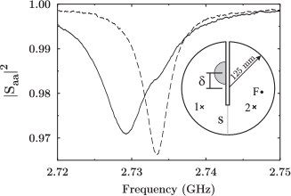
Figure 1: Reflection spectra measured at antenna $1$ (solid) and $2$ (dashed) for $s=1.66~{}{\rm mm}$, $\delta=41.50~{}{\rm mm}$ and ${\rm B}=53~{}{\rm mT}$. Each antenna couples to predominantly one eigenmode for that choice of parameters. We observe a single resonance at antenna 2, a much broader with a shoulder at the peak position of the former at antenna 1. Thus one eigenmode is localized in the right part of the cavity, whereas the second one penetrates from the left into the right part of the cavity. Inset: top view (to scale) of the microwave cavity. In each half of the resonator an antenna, $1$ and $2$, is positioned. A semicircular Teflon disk (gray) is positioned at a distance $\delta$ from the center, $s$ refers to the height of the opening (gray bar) between both cavity parts. A ferrite is located at $F$.

The opening allows a coupling of the electric field modes excited in each half circle, which is varied with a movable gate of copper of length 80 mm and width 3 mm inserted through a small opening in the top plate and operated by a micrometer stepper motor. The bottom of this gate is tilted to allow a precise setting of small couplings. When closing the gate it eventually plunges into a notch in the bottom plate. Its lifting $s$ defines one parameter with the range $0~{}{\rm mm\ (no\ coupling)}\leq s\leq 9~{}{\rm mm\ (full\ coupling)}$. The left half of the circular cavity in Fig. 1 contains a movable semicircular Teflon piece with diameter 60 mm and height 5 mm connected to the outside by a thin snell operated by another stepper motor. Its displacement with respect to the center of the cavity defines the other parameter $\delta$.

Two pointlike dipole antennas intrude into each part of the cavity. A vectorial network analyzer (VNA) Agilent PNA 5230A couples microwave power into the cavity through one antenna $a$ and measures amplitude and phase of the signal received at the same (reflection measurement) or the other (transmission measurement) antenna $b$ relative to the input signal. In this way the complex element $S_{ba}$ of the scattering matrix $S$ is determined. To induce ${\mathcal{T}}\,$violation, a ferrite with the shape of a cylinder of diameter 4 mm and height 5 mm Schaefer2007 is placed in the right part of the cavity and magnetized from the outside by two permanent magnets. They are mounted to a screw thread mechanism above and below the resonator and magnetic field strengths $0~{}{\rm mT}\leq{\rm B}\leq 90~{}{\rm mT}$ are obtained by varying their distance. To automatically scan the parameter space spanned by $(s,\delta)$, the two stepper motors and the VNA are controlled by a PC. The four $S$-matrix elements $S_{ba}(f)$, $\{a,b\}\in\{1,2\}$ are measured in the parameter plane with the resolution $\Delta s=\Delta\delta=0.01~{}{\rm mm}$ and a frequency step $\Delta f=10~{}{\rm kHz}$. The frequency range of 40 MHz is determined by the spread of the resonance doublet. Lack of reciprocity, i.e. $S_{12}\neq S_{21}$, is the signature for ${\mathcal{T}}\,$violation Schaefer2007 . Figure 1 shows two typical reflection spectra, i.e. $|S_{aa}|^{2}$ with $a=1,2$. Additional measurements include neighboring resonances, which are situated about $250~{}{\rm MHz}$ away from the region of interest, in order to account for their residual influence. In the considered frequency range the electric field vector is perpendicular to the top and bottom plates. Then, the Helmholtz equation is identical to the Schrödinger equation for a quantum billiard of corresponding shape QB ; Richter . Consequently, the results provide insight into the associated quantum problem.

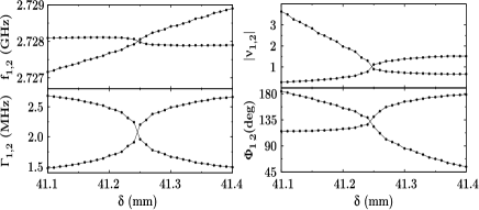
Figure 2: Left panels: Real and imaginary parts of the eigenvalues, $f_{1,2}$ and $\Gamma_{1,2}$, as function of $\delta$ at $s=s_{EP}=1.66~{}{\rm mm}$ and ${\rm B}=53~{}{\rm mT}$. Around $\delta=\delta_{EP}=41.25~{}{\rm mm}$ they are closest. Right panels: Modulus and phase of the ratios $\nu_{1,2}=|\nu_{1,2}|e^{i\Phi_{1,2}}$ of the components of the associated eigenvectors. They are also closest at $\delta\simeq 41.25$ mm. For $\delta\leq\delta_{EP}$ the upper curves correspond to, respectively $f_{1},\,\delta_{1},\,|\nu_{2}|,\,\Phi_{2}$.

In previous experiments D01 ; Dembo2003 an EP was located by determining for each parameter setting the real and imaginary parts of the eigenvalues as the frequencies $f_{1,2}$ and the widths $\Gamma_{1,2}$ of the resonances from a fit of a Breit-Wigner function. This procedure, however, fails at the EP because there the line shape is not a first order pole of the $S$ matrix but rather the sum of a first and a second order pole Metz ; R08 . Therefore, the coalescence of the eigenvectors should be incorporated in the search for the EP Dembo2003 ; Metz . For this we determine the two-state Hamiltonian $H$ and its eigenvalues and eigenvectors explicitely for every setting of the parameters $s,\delta,{\rm B}$ from the measured $S$-matrix elements via the method presented in Schaefer2007 . There, we showed that for a resonator with two pointlike antennas a resonance doublet is well described by the two-channel $S$ matrix $S(f)=\boldsymbol{1}-2\pi iW^{\dagger}(f\,\boldsymbol{1}-H)^{-1}W\,$. The matrix $W=(W_{\mu a})$ couples the resonant states $\mu=1,2$ to the antennas $a=1,2$. It is real since that coupling conserves ${\mathcal{T}}\,$. The Hamiltonian $H$ comprises dissipation in the walls of the resonator and the ferrite and ${\mathcal{T}}\,$violation and thus is neither Hermitian nor symmetric, which implies $S_{12}\neq S_{21}$. Its general form is given as

$$H=\left(\begin{array}[]{cc}e_{1}&H^{S}_{12}-iH^{A}_{12}\\ H^{S}_{12}+iH^{A}_{12}&e_{2}\end{array}\right)\,.$$ (1)

The quantities $e_{1}\pm e_{2},H^{S}_{12}$ and $H^{A}_{12}$ are complex expansion coefficients with respect to the unit and the Pauli matrices. The ansatz for $S$ was tested thoroughly by fitting it to $S$-matrix elements measured with and without magnetization of the ferrite. In the latter case the antisymmetric part $H^{A}_{12}$ vanishes and $H$ coincides with that used in D01 ; Dembo2003 . Fitting the $S$ matrix to the four measured excitation functions $S_{ba}(f)$ yields the matrices $H$ and $W$ up to common real orthogonal basis transformations. We define the basis such that $(H^{S}_{12}+iH^{A}_{12})/(H^{S}_{12}-iH^{A}_{12})=\exp(2i\tau)$ is a phase factor. Thus, ${\mathcal{T}}\,$violation is expressed by a real phase $\tau$. This is usual practice in physics, e.g., for nuclear reactions Driller , and for weak and electromagnetic decay Ri75 .

The eigenvalues of $H$ in Eq. (1) coalesce to an EP when ${H^{S}_{12}}^{2}+{H^{A}_{12}}^{2}+(e_{1}-e_{2})^{2}/4=0$ but not all three terms equal to zero. Figure 2 shows one example for a search of the EP. Keeping $s,{\rm B}$ fixed at $s=1.66$ mm and ${\rm B}=53$ mT, the real and imaginary parts of the eigenvalues, $f_{j}$ and $\Gamma_{j}$ are shown as functions of $\delta$. At $\delta=41.25$ mm the encounter of the eigenvalues is closest. To determine the parameter values for the coalescence of the eigenvectors $|r_{k}\rangle,\,\,k=1,2,$ their components $r_{k1},r_{k2}$ and the ratios $\nu_{k}=r_{k1}/r_{k2}=|\nu_{k}|e^{i\Phi_{k}}$ are determined BD03 . The right part of Fig. 2 demonstrates that the encounter of the eigenvectors is also closest at $\delta=41.25$ mm. Indeed, as will be evidenced in further tests below, both the eigenvalues and the eigenvectors cross at these parameter values. The EP is located at $(s_{EP},\delta_{EP})=(1.66\pm 0.01,41.25\pm 0.01)$ mm. At the EP the only eigenvector of $H$ is HH04

$$|r_{\rm EP}\rangle=\left(\begin{array}[]{c}i\,e^{i\tau}\\ 1\end{array}\right)\,.$$ (2)

The ratio of its components is a phase factor. For ${\mathcal{T}}$-conserving systems the phase is $\Phi_{\rm EP}=\pi/2$ Dembo2003 as confirmed by Fig. 3 at ${\rm B}=0$. With ${\mathcal{T}}\,$violation the phase equals $\Phi_{\rm EP}=\tau+\pi/2$ and thus provides a measure for its size $\tau$. Figure 3 shows that with increasing ${\rm B}$ the parameter $\tau$ goes through a maximum. As in Ref. Schaefer2007 we identify this with the ferromagnetic resonance resulting from the coupling of the rf magnetic field to the spins in the ferrite. The ${\mathcal{T}}$-violating matrix element $iH^{A}_{12}$ has been expressed by a resonance formula which yields the solid curve for $\Phi_{\rm EP}({\rm B}$).

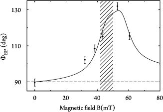
Figure 3: Phase of the ratio $\nu_{EP}$ of the eigenvector components at the EP as a function of the magnetization of the ferrite. For the ${\mathcal{T}}$-conserving case the known result Dembo2003 of $90^{\circ}$ (dashed horizontal line) is recovered. The model for the ${\mathcal{T}}$-violating matrix element $iH^{A}_{12}$ in terms of the ferromagnetic resonance yields the solid line which agreeably describes the data. The vertical bar indicates the range of ${\rm B}$ where the ferromagnetic resonance is expected.

Panel (a) of Fig. 4 shows in a neighborhood of the EP at ${\rm B}=53$ mT the differences of the complex eigenvalues, $f_{1,2}$ (blue, left to EP) and $\Gamma_{1,2}$ (orange, right to EP), panel (b) those of the phases $\Phi_{1,2}$ (orange, left to EP) and of the moduli $|\nu_{1,2}|$ (green, right to EP). The darker the colour the smaller is the respective difference. The darkest colour visualizes the curve (branch cut) along which it vanishes. The left and right panels of Fig. 2 are cuts through the respective panels of Fig. 4 at $s=1.66$ mm. We observe that $|f_{1}-f_{2}|$ and $|\Phi_{1}-\Phi_{2}|$ are small and thus visible only to the left of the EP, whereas $|\Gamma_{1}-\Gamma_{2}|$ and $||\nu_{1}|-|\nu_{2}||$ are visible only to its right. Thus the branch cuts all extend from one common point into opposite directions. This proves that this point is an EP BD03 ; MF80 ; Lee2009 .

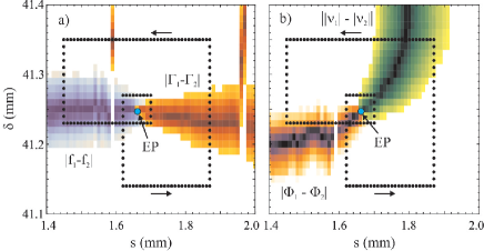
Figure 4: Differences of the complex eigenvalues $f_{1,2}+i\Gamma_{1,2}$ (a) and of the ratios $\nu_{1,2}=|\nu_{1,2}|e^{i\Phi_{1,2}}$ of the eigenvector components (b) in an area of the parameter plane $(s,\delta)$ around the EP. The darker the colour the smaller is the respective difference. That of $f_{1,2}$ (blue) and of $\Phi_{1,2}$ (orange) are small only to the left, those of $\Gamma_{1,2}$ (orange) and of $|\nu_{1,2}|$ (green) to the right of the EP. The black dots in both panels indicate the chosen contour for the encircling of the EP (see text).

For systems with ${\mathcal{T}}\,$violation the geometric phase $\gamma$ gathered by the eigenvectors around an EP is predicted to be complex yielding a geometric amplitude $e^{-{\rm Im}\gamma}\neq 1$ GW88 . To check this we choose contours around the EP for the six values of the magnetic field ${\rm B}$ considered in Fig. 3. One example is shown in Fig. 4. As proposed in MM08 it consists of two different loops. The path is parametrized by a real variable $t$ with initial value $t=0$. In Dubbers and D01 the geometric phase gathered around a DP, respectively an EP, was obtained for just a few parameter settings, because the procedure – the measurement of the electric field intensity distribution – is very time consuming. We now have the possibility to determine the left and right eigenvectors, $\langle l_{j}(t)|$ and $|r_{j}(t)\rangle,\,j=1,2$ of $H$ in Eq. (1) on a much narrower grid of the parameter plane. At each point $t$ of the contour they are biorthonormalized, such that $\langle l_{j}(t)|r_{j}(t)\rangle=1$. Defining in analogy to the ${\mathcal{T}}$-conserving case D01 $\mathcal{B}=\frac{(e_{1}-e_{2})}{2}/\sqrt{{H^{S}_{12}}^{2}+{H^{A}_{12}}^{2}},\,\tan\theta=\sqrt{1+\mathcal{B}^{2}}-\mathcal{B}$ yields for the right eigenvectors GW88

$$|r_{1}(t)\rangle=\left(\begin{array}[]{c}e^{-i\tau/2}\cos\theta\\ e^{i\tau/2}\sin\theta\end{array}\right),\,|r_{2}(t)\rangle=\left(\begin{array}[]{c}-e^{-i\tau/2}\sin\theta\\ e^{i\tau/2}\cos\theta\end{array}\right)\,.$$ (3)

As in D01 the EPs are located at $1+\mathcal{B}^{2}=0$ and encircling the EP once changes $\theta$ to $\theta\pm\pi/2$. The ${\mathcal{T}}$-violating parameter $\tau$ is not constant along the contour, even though the magnetic field is fixed. In fact, it varies with the opening $s$ between both parts of the resonator, because the ferrite is positioned in one of them, see Fig. 1. The position of the EP does not depend on the value of $\tau$. Thus, the space curve $(s(t),\delta(t),\tau(t))$ winds around the line $(s_{EP},\delta_{EP},\tau(t))$, see Ref. MKS05 . Since $\tau$ has no singular points in the considered parameter plane it returns to its initial value after each encircling of the EP. As a consequence, the eigenvectors $|r_{1,2}(t)\rangle$ follow the same transformation scheme as in the ${\mathcal{T}}$-conserving case. After completing the first loop at $t=t_{1}$ we have $|r_{1}(t_{1})\rangle=|r_{2}(0)\rangle$, $|r_{2}(t_{1})\rangle=-|r_{1}(0)\rangle$ and after the second one at $t=t_{2}$ we find $|r_{1,2}(t_{2})\rangle=-|r_{1,2}(0)\rangle$.

The biorthonormality defines the eigenvectors $\langle l_{j}|$ and $|r_{j}\rangle$ up to a geometric factor, so that $\langle L_{j}(t)|=\langle l_{j}(t)|\,e^{-i\gamma_{j}(t)}$ and $|R_{j}(t)\rangle=|r_{j}(t)\rangle\,e^{i\gamma_{j}(t)}$. The geometric phases $\gamma_{j}(t)$ are fixed by the condition of parallel transport B84 ; GW88 ; FN , $\left\langle L_{j}(t)|\frac{\rm d}{{\rm d}t}R_{j}(t)\right\rangle=0$. This yields $\frac{{\rm d}\gamma_{1}(t)}{{\rm d}t}=\frac{1}{2}\cos 2\theta(t)\frac{{\rm d}\tau(t)}{{\rm d}t}=-\frac{{\rm d}\gamma_{2}(t)}{{\rm d}t}$. The initial value of the phases is chosen as $\gamma_{j}(0)=0$, such that $\gamma_{1}(t)=-\gamma_{2}(t)$. For the ${\mathcal{T}}$-conserving case we find $\gamma_{1,2}(t)\equiv 0$. The phase $\gamma_{1}(t)$ is determined successively for increasing $t$ from the product of $\langle l_{1}(t)|$ and $\left|\frac{\rm d}{{\rm d}t}r_{1}(t)\right\rangle$. In the upper panel of Fig. 5 is plotted the phase $\gamma_{1}(t)$ accumulated by $|R_{1}(t)\rangle$ when encircling the EP twice along the outer loop of the contour in Fig. 4. The lower panel shows $\gamma_{1}(t)$ for the contour in Fig. 4. The start point is the intersection of the loops. The orientation is chosen such that the EP is always to the left. The cusps occur where $\frac{{\rm d}\tau}{{\rm d}t}=0$. In each panel the triangle marks the start point, the pentagon the point $t_{1}$, where the EP is encircled once, the diamond marks the point $t_{2}$ of completion of the second encircling. One sees that in both examples $\gamma_{1}(t_{1})\neq 0$ and that, as predicted in Ref. GW88 , the geometric phase $\gamma_{1}(t_{1})$ is not real. If the EP is encircled twice along the same loop, we obtain $\gamma_{1}(t_{2})=0$ MKS05 ; MM08 within $10^{-7}$. Thus we measured the $\gamma$’s up to an accuracy manifestly better than $10^{-2}$. Accordingly, from the value of $\gamma_{1}(t_{2})$ given in the caption of Fig. 5 we may conclude that, when the loops are different $\gamma_{1}(t)$ does not return to its initial value MM08 . When encircling this double loop again and again we observe a drift of $\gamma_{1,2}$ in the complex plane away from the origin. Thus, one geometric amplitude increases and the other one decreases. This provides the experimental proof for the existence of a reversible geometric pumping process, as predicted in GW88 . The dependence on the choice of the path signifies that the complex phases $\gamma_{1,2}(t)$ are geometric and not topological. In order to obtain the complete phase gathered by $|R_{1}(t)\rangle$ during the encircling of the EP one has to add the topological phase accumulated by $|r_{1}(t)\rangle$.

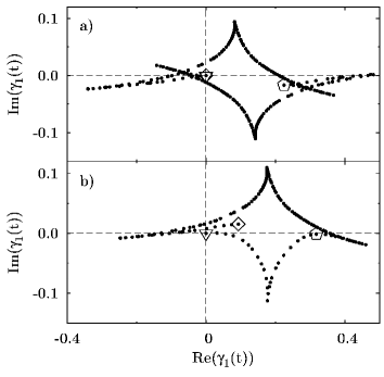
Figure 5: The complex phase $\gamma_{1}(t)$ for ${\rm B}=53~{}{\rm mT}$ when encircling the EP twice along the outer loop (upper panel), and along the inner and outer loops (lower panel) of the contour shown in Fig. 4. The triangle marks the start point, the pentagon the point after encircling the EP once ($t=t_{1}$), the diamond that after a second encircling ($t=t_{2}$). There, $\gamma_{1}(t_{2})$ equals $(3.123-i3.474)\cdot 10^{-7}$, i.e. it is close to zero in the upper case, $0.0931+i0.0152$ in the lower one.

In summary, when encircling the EP we obtain geometric factors different from unity and the transformation scheme Eq. (3) for $|\vec{r}_{1,2}(t)\rangle$. These results provide an unambiguous proof that the EP lies inside both loops of the contour shown in Fig. 4. Their precision is illustrated by the dense sequence of points in Fig. 5. The accuracy of the measurements at and around the EP allows the determination of the size of ${\mathcal{T}}\,$violation and of the geometric factor along arbitrary contours in the parameter plane. Predictions on geometric amplitudes and phases could be confirmed.

- (1) J. C. Garrison and E. M. Wright, Phys. Lett. A, 128, 177 (1988); M. V. Berry, Proc. R. Soc. Lond. A 430, 405 (1990); K. Yu. Bliokh, J. Math. Phys., 32, 2551 (1999).
- (2) N. Moiseyev and S. Friedland, Phys. Rev. A 22, 618 (1980); W. D. Heiss and A. L. Sannino, J. Phys. A 23, 1167 (1990); E. Hernandez, A. Jauregui, A. Mondragon, J. Phys. A: Math. Gen. 33, 4507 (2000); A. P. Seyranian, O. N. Kirillov, and A. A. Mailybaev, J. Phys. A 38, 1723 (2005).
- (3) H. L. Harney and W. D. Heiss, Eur. Phys. J. D 29, 429 (2004); W. D. Heiss, J. Phys. A 39, 10077 (2006).
- (4) I. Rotter, J. Phys. A: Math. Theor. 42, 153001 (2009).
- (5) M. V. Berry, Proc. R. Soc. Lond. A 392, 45 (1984); A. Bohm et al., The Geometric Phase in Quantum Systems (Berlin: Springer) 2003.
- (6) M. V. Berry and M. R. Dennis, Proc. R. Soc. Lond. A. 459, 1261 (2003).
- (7) T. Kato, Perturbation Theory for Linear Operators (Berlin: Springer) 1966.
- (8) O. Latinne, N.J. Kylstra, M. Dorr, et al., Phys. Rev. Lett. 74, 46 (1995); E. Narevicius, N. Moiseyev, Phys. Rev. Lett. 84, 1681 (2000); H. A. Weidenmüller, Phys. Rev. B, 68, 125326 (2003); H. Cartarius, J. Main, G. Wunner, Phys. Rev. Lett. 99, 173003 (2007); P. Cejnar, S. Heinze, M. Macek, Phys. Rev. Lett. 99, 100601 (2007); R. Lefebvre, O. Atabek, M. Sindelka, and N. Moiseyev, Phys. Rev. Lett. 103, 123003 (2009); R. Lefebvre and O. Atabek, Eur. Phys. J. D. 56, 317 (2010).
- (9) J. Wiersig, S. W. Kim, and M. Hentschel, Phys. Rev. A 78, 053809 (2008); J.-W. Ryu, S.-Y. Lee, S. W. Kim, Phys. Rev. A 79, 053858 (2009); A. C. Or, Quart. J. Mech. Appl. Math. 44, 559 (1991); M. Kammerer, F. Merz, F. Jenko, Phys. Plasmas 15, 052102 (2008); O. N. Kirillov, Proc. R. Soc. A 464, 2321 (2008); S. Klaiman, U. Günther, N. Moiseyev, Phys. Rev. Lett. 101, 080402 (2008); Ch. E. Ruter et al., Nature Physics 6, 192 (2010).
- (10) M. Philipp, P. von Brentano, G. Pascovici, and A. Richter, Phys. Rev. E 62, 1922 (2000).
- (11) C. Dembowski et al., Phys. Rev. Lett. 86, 787 (2001); Phys. Rev. E, 69, 056216 (2004).
- (12) C. Dembowski et al., Phys. Rev. Lett. 90, 034101 (2003).
- (13) B. Dietz et al., Phys. Rev. E 75, 027201 (2007).
- (14) H.-J. Stöckmann and J. Stein, Phys. Rev. Lett. 64, 2215 (1990); H.-D. Gräf et al., Phys. Rev. Lett. 69, 1296 (1992).
- (15) T. Stehmann, W. D. Heiss, F. G. Scholtz, J. Phys. A: Math. Gen. 37, 7813 (2004).
- (16) S.-B. Lee et al., Phys. Rev. Lett. 103, 134101 (2009); Y. Choi et al., Phys. Rev. Lett. 104, 153601 (2010).
- (17) B. Dietz et al., Phys. Rev. Lett. 98, 074103 (2007).
- (18) F. Haake, Quantum Signatures of Chaos (Springer, New York, 2001)
- (19) A. A. Mailybaev, O. N. Kirillov, A. P. Seyranian, Phys. Rev. A 72, 014104 (2005); Dokl. Math. 73, 129 (2006).
- (20) H. Mehri-Dehnavi and A. Mostafazadeh, J. Math. Phys., 49, 082105 (2008).
- (21) A. Richter, in Emerging Applications of Number Theory, edited by D.A. Hejhal et al., The IMA Volumes of Mathematics and its Applications Vol. 109 (Springer, NY 1999), p. 479; H.-J. Stöckmann, Quantum Chaos: An Introduction (Cambridge University Press, Cambridge, 2000).
- (22) H. Driller et al., Nuc. Phys. A 317, 300 (1979); J.M. Pearson and A. Richter, Phys. Lett. B 56, 112 (1975).
- (23) A. Richter, in Interaction Studies in Nuclei, ed. by H. Jochim and B. Ziegler, (North-Holland, Amsterdam 1975) p. 191.
- (24) H.-M. Lauber, P. Weidenhammer and D. Dubbers, Phys. Rev. Lett. 72, 1004 (1994).
- (25) Note that previous numerical studies did not use biorthonormalized eigenvectors in the parallel transport. The thus obtained geometric factors differ from the present ones without contradicting them.