Generation of entanglement density within a reservoir

Abstract

We study a single two-level atom interacting with a reservoir of modes defined by its reservoir structure function. Within this framework we are able to define a density of entanglement involving a continuum of reservoir modes. The density of entanglement is derived for a system with a single excitation by taking a limit of the global entanglement. Utilizing the density of entanglement we quantify the entanglement between the atom and the modes, and also between the reservoir modes themselves.

I Introduction

In recent years, entanglement has attracted the attention of many physicists working in the area of quantum mechanics Amico2008 ; Horodecki2009 . This is due to the ongoing research in the area of quantum information Nielsen , and also because of the advances made in different experimental disciplines, such as in ion traps Leibfried2003 and Bose-Einstein condensation Dalfovo1999 ; Leggett2001 . Developments in the field of cavity QED, where experiments in the strong coupling regime are carried out Raimond2001 ; Varcoe2004 provide plenty of motivation for studying quantum information and entanglement. Theoretical studies are also important in the context of atom-light interactions inside structured reservoirs Lambropoulos2000 such as resonant cavities or photonic band gap materials. The theoretically predicted atom-photon bound state could also lead to entanglement and this can also be linked to another problem: that of atom-laser out-coupling from Bose-Einstein condensates Nikolopoulos2003 ; Lazarou2007 ; Nikolopoulos2008 , where analogous effects were predicted in the past.

In a recent work by Cummings and Hu CummingsN2008 , a two-level atom coupled to a large reservoir was considered. Starting with simple models with a few modes, they generalize to reservoirs with a large number of modes, where they examine entanglement between the atom and the reservoir. In their analysis the reservoir is treated as a collective object, i.e. the entanglement between the atom and each mode, or between the modes, is not considered.

In the present work we study entanglement between the atom and the reservoir by means of a different approach. In our model, an atom interacts with a continuum of modes at zero temperature Haroche ; Breuer , and entanglement properties between the atom and the modes and also between the modes are considered. Using global entanglement as a measure of entanglement, we derive a pair of distributions that can be interpreted as densities of entanglement in terms of all the reservoir modes. Both distributions can be calculated in terms of the spectrum of reservoir excitation. With these two new measures of entanglement we can study in detail entanglement between the atom and the modes, and also between the modes.

In our analysis, we consider a Lorentzian reservoir and cover different dynamic regimes. For strong coupling we observe the periodic collapses and revivals of entanglement between the atom and the reservoir, which are associated with Rabi oscillations of the atom. Eventually, all the population leaves the atom and the reservoir becomes entangled. More precisely, two bundles of modes are excited, forming a “Bell-like” state. The method developed here, in terms of entanglement distributions, can also be used when considering various types of structured reservoirs. For example, reservoirs with a density of modes characterized by a band gap Garraway1997a ; Garraway1997b ; Lambropoulos2000 can be treated with this method.

The paper is organized as follows. In section II we introduce a measure of entanglement, the global entanglement, and apply it to our system-reservoir states when the number of degrees of freedom is finite. In section III we introduce the density of entanglement for the limit of a bath with an infinite number of modes. This entanglement measure evolves according to our model system as introduced in section IV. In section V we present our key results for the density of entanglement and we conclude in section VI.

II Measures of multi-partite entanglement

Identifying and measuring entanglement in multi-partite systems presents various complications. Apart from the case of a two-qubit system, where entanglement can be identified both for a pure and a mixed state Hill1997 ; Wootters1998 , multi-qubit entanglement is an open problem and to date several measures of entanglement have been proposed Amico2008 ; Horodecki2009 ; Mintert2005a ; Barnum2004 ; Meyer2002 ; Aktharshenas2005 . For the analysis that follows we will be using the global entanglement Meyer2002 since this will enable us to deal with many modes (or qubits). The physical problem we consider is that of entanglement between an atom and a reservoir, and in the context of this problem we will also consider the entanglement between different reservoir modes. To quantify this we will take a discrete bath of reservoir modes. Since we will assume only a single excitation in each bath mode, we can treat the bath states as a set of qubits for the purpose of computing the entanglement, and then later take a continuum limit. With just one excitation in total in the system, this excitation may be in the atom, or in the bath, so that the state vector at all times will have the form

$$|\psi(t)\rangle=c_{0}|\textbf{0}\rangle+c_{a}(t)|\psi_{a}\rangle+\sum_{\lambda}c_{\lambda}(t)|\psi_{\lambda}\rangle,$$ (1)

where $|\textbf{0}\rangle$ is the vacuum state

$$|\textbf{0}\rangle=|0\rangle_{a}\otimes|0000\cdots 000\rangle.$$ (2)

The other two states $|\psi_{a}\rangle$ and $|\psi_{\lambda}\rangle$, correspond to the atom being excited

$$|\psi_{a}\rangle=|1\rangle_{a}\otimes|000\cdots 000\rangle,$$ (3)

or the mode $\lambda$ of the reservoir being excited

$$|\psi_{\lambda}\rangle=|0\rangle_{a}\otimes|000\cdots 01_{\lambda}0\cdots 000\rangle.$$ (4)

Recently this kind of approach has been utilized for the study of decoherence and entanglement decay in systems with one or two excitations (effectively at $T=0$) Bellomo07 ; Bellomo08 ; Maniscalco08 ; Wang08 ; Fussel08 ; Thanopoulos08 ; Alamri09 ; Li09 ; Mazzola09a ; Mazzola10b ; Zhou09 ; Ferraro09 ; Francica09 ; Xiao09 ; Zhang09 ; Mazzola09c ; Mazzola09b ; He10 ; Zhang10a ; Man10 ; Zhou10 ; Zhang10b ; Ge10 ; Mazzola10a ; Tong10b ; Wang10 ; Tong10a ; Fanchini10 ; HamadouIbrahim10 ; Li10 ; Xu10 . Some of this work examines the decay of a single excitation in a reservoir made from a continuum of modes Fussel08 ; Thanopoulos08 ; Mazzola09b ; Tong10a and other works examine entaglement with two or more qubits, but most still utilize the decay of a single excitation as considered in the present paper Bellomo07 ; Bellomo08 ; Maniscalco08 ; Wang08 ; Li09 ; Mazzola09a ; Mazzola10b ; Zhou09 ; Ferraro09 ; Francica09 ; Xiao09 ; Zhang09 ; Mazzola09c ; Ge10 ; Tong10b ; Wang10 ; Man10 ; Zhou10 ; Alamri09 ; He10 ; Zhang10a .

If we started with a system of $N$ qubits in a pure state $|\psi\rangle$, the global entanglement is defined as

$$Q(|\psi\rangle)=2-\frac{2}{N}\sum_{i=1}^{N}\textrm{tr}\rho^{2}_{i},$$ (5)

where $\rho_{i}$ is the reduced density matrix for the $i$-th qubit. When $|\psi\rangle$ is a pure product state then $Q(|\psi\rangle)=0$. If we take an entangled state for $|\psi\rangle$, such as the GHZ state

$$|GHZ\rangle_{N}=(|000\cdots\rangle+|111\cdots\rangle)/\sqrt{2},$$ (6)

then $\textrm{Q}(|\psi\rangle)=1$. This example gives a maximum value for the global entanglement which is normalized such that $0\leq Q(|\psi\rangle)\leq 1$. Another, more relevant example is the W-state

$$|W\rangle_{N}=\sum_{j=1}^{N}|0\cdots 01_{j}0\cdots 0\rangle/\sqrt{N},$$ (7)

for which the global entanglement goes to zero as $1/N$ for large $N$

$$\textrm{Q}(|\psi\rangle)=4(N-1)/N^{2}.$$ (8)

An important property of the global entanglement is that it is equal to a sum over two-qubit concurrences Horodecki2009 . More specifically, for pure states $|\psi(t)\rangle$ [Eq. (1)] we find from Eq. (5), see the appendix for details, that

$$Q(|\psi\rangle)=\frac{2}{N+1}C^{2}(t),$$ (9)

where $C^{2}(t)$ reads

$$C^{2}(t)=\sum_{\lambda=1}^{N}c^{2}(\rho_{a\lambda})+\sum_{1\leq\lambda<\mu\leq N}c^{2}(\rho_{\lambda\mu}).$$ (10)

The concurrence $c^{2}(\rho_{a\lambda})$ is that for the two-qubit (reduced) density matrix $\rho_{a\lambda}$ Hill1997 ; Wootters1998

$$\rho_{a\lambda}=\textrm{tr}_{\mu\neq\lambda}\left\{|\psi(t)\rangle\langle\psi(t)|\right\}$$ (11)

between the atom and the $\lambda$-mode. The quantity $\rho_{\mu\lambda}$ is the corresponding density matrix for the modes $\mu$ and $\lambda$:

$$\rho_{\mu\lambda}=\textrm{tr}_{a,\kappa\neq\lambda,\mu}\left\{|\psi(t)\rangle\langle\psi(t)|\right\}.$$ (12)

The two-qubit concurrence $c(\rho)$ is equal to Hill1997 ; Wootters1998

$$c(\rho)=\textrm{max}\{0,\sqrt{\lambda_{1}}-\sqrt{\lambda_{2}}-\sqrt{\lambda_{3}}-\sqrt{\lambda_{4}}\},$$ (13)

where $\lambda_{j}$ are the eigenvalues of the matrix

$$R=\rho(\sigma_{y}\otimes\sigma_{y})\rho^{\ast}(\sigma_{y}\otimes\sigma_{y}),$$ (14)

in decreasing order, i.e. $\lambda_{1}>\lambda_{2}>\lambda_{3}>\lambda_{4}$, and $\sigma_{y}$ is the relevant Pauli matrix.

Is is important to note here that $C^{2}(t)$ is exactly equal to the square of the norm of the concurrence vector Aktharshenas2005 , which is one of the many proposed measures for multi-partite entanglement. Because of the connection between $C^{2}(t)$ and the two-qubit concurrence Eq. (10), we shall refer to $C^{2}(t)$ simply as the concurrence.

For the remainder of this work we will focus only on $C^{2}(t)$ and its properties since, with the exception of the normalization factor $2/(N+1)$ in Eq. (9), it is equivalent to the global entanglement. Furthermore, we will be considering a continuum of reservoir modes, i.e. $N\gg 1$. In this limit, as we see in the following section, one can define a density of entanglement for continuous systems.

III Density of entanglement

In the limit of continuous distribution for the reservoir modes, the summations in Eq. (10) can be converted into integrals over the density of modes $\rho_{\lambda}$, i.e.

$$\sum_{\lambda}\rightarrow\int\textrm{d}\omega_{\lambda}\rho_{\lambda}.$$ (15)

If we take this limit, the concurrence $C^{2}(t)$ can be expressed as the sum of two separate parts which ultimately involve either atomic population or reservoir mode populations:

$$\begin{split}C^{2}(t)=&\int_{-\infty}^{\infty}d\omega_{\lambda}\mathcal{E}_{A}(\omega_{\lambda},t)\\ \\ &+\int_{-\infty}^{\infty}d\omega_{\lambda}\int_{-\infty}^{\infty}d\omega_{\mu}\mathcal{E}_{R}(\omega_{\lambda},\omega_{\mu},t).\end{split}$$ (16)

The two distributions $\mathcal{E}_{A}$ and $\mathcal{E}_{R}$ will form the entanglement densities and are defined in terms of the two qubit concurrences to be

$$\mathcal{E}_{A}(\omega_{\lambda},t)=c^{2}(\rho_{a\lambda})\rho(\omega_{\lambda}),$$ (17)

and

$$\mathcal{E}_{R}(\omega_{\lambda},\omega_{\mu},t)=\frac{1}{2}c^{2}(\rho_{\lambda\mu})\rho(\omega_{\lambda})\rho(\omega_{\mu}),$$ (18)

where $\rho(\omega)$ is the reservoir density of modes. The interpretation for these two functions is now very simple.

The distribution $\mathcal{E}_{A}(\omega_{\lambda},t)$ is the density of entanglement between the atom and all reservoir modes in the vicinity of mode $\omega_{\lambda}$ i.e.  $\mathcal{E}_{A}(\omega_{\lambda},t)\textrm{d}\omega_{\lambda}$ is the total entanglement between the atom and all modes in the frequency interval $\omega_{\lambda}$ and $\omega_{\lambda}+\textrm{d}\omega_{\lambda}$. In the same way $\mathcal{E}_{R}(\omega_{\lambda},\omega_{\mu},t)\textrm{d}\omega_{\mu}$ gives the entanglement between the mode $\omega_{\lambda}$ and modes in the frequency range $\omega_{\mu}$ to $\omega_{\mu}+\textrm{d}\omega_{\mu}$.

For the remainder of this work, $\mathcal{E}_{A}$ will be referred as the atom-mode density of entanglement and to $\mathcal{E}_{R}$ as the mode-mode density of entanglement. The global entanglement $Q(|\psi\rangle)$, Eq. (9), can be calculated from these two densities of entanglement, and thus a number of entanglement properties can be studied in terms of these two distributions. To this end it is important to note an interesting property for the two distributions $\mathcal{E}_{A}$ and $\mathcal{E}_{R}$. One can show that both entanglement distributions can be written in terms of the spectrum of reservoir excitation Linington2006

$$S(\omega_{\lambda},t)=\rho(\omega_{\lambda})|c_{\lambda}(t)|^{2},$$ (19)

as

$$\mathcal{E}_{A}(\omega_{\lambda},t)=4|c_{a}(t)|^{2}S(\omega_{\lambda},t),$$ (20)

and

$$\mathcal{E}_{R}(\omega_{\lambda},\omega_{\mu},t)=2S(\omega_{\lambda},t)S(\omega_{\mu},t)\,.$$ (21)

Thus, both entanglement distributions can be derived from the reservoir excitation spectrum. Having the definition for the entanglement density we can now introduce a Hamiltonian and dynamics to consider the time-dependent properties of entanglement for an atom coupled to a Lorentzian reservoir.

IV Dynamical model

The model system consists of a two-level atom coupled to a reservoir of harmonic oscillators with annihilation and creation operators $a_{\lambda}$ and $a_{\lambda}^{\dagger}$ respectively. Within the rotating wave approximation the Hamiltonian reads $(\hbar=1)$

$$\begin{split}H=&\sum_{\lambda}\omega_{\lambda}a_{\lambda}^{\dagger}a_{\lambda}+\omega_{0}|1\rangle_{aa}\langle 1|\\ \\ &+\sum_{\lambda}g_{\lambda}\left(a_{\lambda}^{\dagger}|0\rangle_{aa}\langle 1|+a_{\lambda}|1\rangle_{aa}\langle 0|\right),\end{split}$$ (22)

where $g_{\lambda}$ is the coupling between the mode $\lambda$ and the atomic transition $|1\rangle_{a}\rightarrow|0\rangle_{a}$. The atomic transition frequency is $\omega_{0}$ whereas the $\lambda$-mode frequency is $\omega_{\lambda}$. This model will preserve the assumption of a single excitation which is built into the system states in Eq. (1).

For the purposes of the analysis that follows, it is very useful to introduce the reservoir structure function $D(\omega_{\lambda})$ which reflects the properties of the density of modes Garraway1997a . This is defined through

$$\rho_{\lambda}(g_{\lambda})^{2}=\frac{\Omega^{2}_{0}}{2\pi}D(\omega_{\lambda}),$$ (23)

and is normalized such that

$$\int_{-\infty}^{\infty}\textrm{d}\omega D(\omega)=2\pi.$$ (24)

With this normalization a measure of the overall coupling strength is $\Omega_{0}$ which is given by

$$\Omega_{0}^{2}=\sum_{\lambda}(g_{\lambda})^{2}.$$ (25)

Utilizing these assumptions, and a state vector of the form given by Eq. (1), the Schrödinger equation in an interaction picture yields

$$\textrm{i}\frac{\textrm{d}}{\textrm{d}t}\tilde{c}_{a} = \sum_{\lambda}g_{\lambda}e^{-\textrm{i}\delta_{\lambda}t}\tilde{c}_{\lambda},$$ (26)

$$\textrm{i}\frac{\textrm{d}}{\textrm{d}t}\tilde{c}_{\lambda} = g_{\lambda}e^{\textrm{i}\delta_{\lambda}t}\tilde{c}_{a},$$ (27)

with the detuning between the atomic transition and the mode $\lambda$ being given by

$$\delta_{\lambda}=\omega_{\lambda}-\omega_{0}.$$ (28)

The interaction picture amplitudes $\tilde{c}_{a}$ and $\tilde{c}_{\lambda}$ are connected to $c_{a}$ and $c_{\lambda}$ via a time-dependent transformation

$$\tilde{c}_{a}(t)=e^{\textrm{i}\omega_{0}t}c_{a}(t),\quad\tilde{c}_{\lambda}(t)=e^{\textrm{i}\omega_{\lambda}t}c_{\lambda}(t).$$ (29)

Apart from numerical integration of equations (26) and (27), one could use analytical methods to derive the dynamics. Examples of these are: the resolvent method Lambropoulos2000 , the Laplace transform John1994 ; Kofman1994 and that of the pseudomodes Garraway1997a ; Garraway1997b ; Dalton01a ; Mazzola09b . This latter method applies when the spectral function is analytic with poles in the lower complex plane. Then equations (26) and (27) can be replaced, in the continuum limit, by a set of equivalent equations where the atom now couples to a finite set of fictitious modes. Each of these modes has a one–to–one correspondence to the poles of $D(\omega)$.

For concreteness we consider Lorentzian reservoir structure functions of width $\Gamma$ and peak frequency $\omega_{c}$, i.e.

$$D(\omega)=\frac{\Gamma}{(\omega-\omega_{c})^{2}+(\Gamma/2)^{2}}.$$ (30)

This reservoir function has a simple pole at

$$z=\omega_{c}-\textrm{i}\Gamma/2,$$ (31)

and for this $D(\omega)$ equations (26) and (27) are equivalent to two new equations

$$\textrm{i}\frac{\textrm{d}}{\textrm{d}t}\tilde{c}_{a}(t) = \Omega_{0}\tilde{b}(t),$$ (32)

$$\textrm{i}\frac{\textrm{d}}{\textrm{d}t}\tilde{b}(t) = (\Delta-\textrm{i}\Gamma/2)\tilde{b}(t)+\Omega_{0}\tilde{c}_{a}(t),$$ (33)

where the atom-cavity detuning $\Delta=\omega_{c}-\omega_{0}$, and $b(t)=e^{-\textrm{i}\omega_{0}t}\tilde{b}(t)$ is the pseudomode amplitude. This set of equations can be associated with a master equation, where the physical interpretation for the pseudomode is that of a leaking cavity mode coupled to the atomic transition Garraway1997a .

These coupled ODEs are straightforward to solve, and in particular, for the case of resonance, $\omega_{c}=\omega_{0}$, one finds for the atomic amplitude $c_{a}(t)$:

$$\tilde{c}_{a}(t)=\tilde{c}_{a}(0)e^{-\frac{\Gamma t}{4}}\left(\cosh\left(\alpha t/4\right)+\frac{\Gamma}{\alpha}\sinh\left(\alpha t/4\right)\right).$$ (34)

The modified decay rate $\alpha$ is given by

$$\alpha=\sqrt{\Gamma^{2}-(4\Omega_{0})^{2}}$$ (35)

in terms of $\Gamma$ and $\Omega_{0}$. For strong couplings, $4\Omega_{0}/\Gamma\gg 1$, the atomic population oscillates between the atom and the reservoir with a slowly decaying amplitude. In the long time limit all the energy is lost to the reservoir. If we decrease the coupling $\Omega_{0}$, the atom dissipates its energy faster, and for $4\Omega_{0}/\Gamma\ll 1$ the atom exponentially decays into the reservoir. These two types of behavior are illustrated in Fig. 1 which is given as a reference point for the entanglement discussion in the next section. The figures show the atomic population for $\Omega_{0}=10\Gamma$ and $\Omega_{0}=0.1\Gamma$ plotted against time $t$.

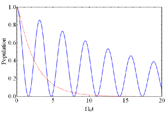
Figure 1: The atomic population $|c_{a}(t)|^{2}$ as a function of time for strong coupling $\Omega_{0}=10\Gamma$ (solid line), and weak coupling $\Omega_{0}=0.1\Gamma$ (dashed line). Both results were obtained from Eq. (34). The initial system state in this and the following figures is defined by $c_{a}(0)=1$, $c_{0}=0$ and all $c_{\lambda}(0)=0$. The detuning $\Delta=0$.

V Evolution of reservoir entanglement

V.1 Entanglement generation by decay

The interaction between the atom and the reservoir results in entanglement creation between the atom and the reservoir modes, and also between the reservoir modes. This latter entanglement is indirect and is due to the effective coupling between the modes as a result of their interaction with the atom. When considering our measure of the total entanglement, the concurrence $C^{2}(t)$ as a function of time (Fig. 2), we see that for both strong and weak coupling the concurrence builds up to a maximum value equal to $C^{2}(t)=2$.

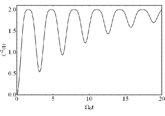
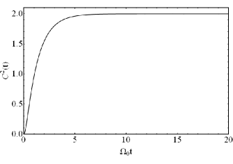
Figure 2: The concurrence $C^{2}(t)$ as a function of time for different couplings $\Omega_{0}=10\Gamma$ (a) and $\Omega_{0}=0.1\Gamma$ (b). The result was obtained from Eqs. (16), (20) and (21).

In the case of strong coupling, Fig. 2, the concurrence reaches the maximum value very quickly, and then oscillates in a way which is closely connected to the Rabi oscillations seen in Fig. 1. The oscillations return to the maximum value of two, with a minimum value that also approaches two as time increases. If we compare the concurrence to the population in Fig. 1 we see that every minimum in concurrence is matched by a peak in population of the atomic state. Likewise the maxima in concurrence are matched by minima in the atomic population: it seems that the decaying atom is very efficient at generating entanglement in the reservoir. At this point we note that at long times the energy has left the atom (see the population Fig. 1) and the system is in an approximate product state of unexcited atom and bath states. The large value of the concurrence at these times indicates the presence of entanglement in the bath. In the long time limit the concurrence reaches a steady value $C^{2}(\infty)=2$, a result that can be derived analytically if one uses Eqs. (16) (20) and (21) and the spectrum for $t\rightarrow\infty$. This limit for the concurrence is the same in the weak coupling case, see Fig. 2; the atom decays exponentially and the entanglement reaches a steady state monotonically. In the long time limit the atom again disentangles from the reservoir and entanglement is distributed only between the reservoir modes.

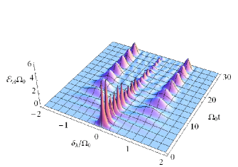
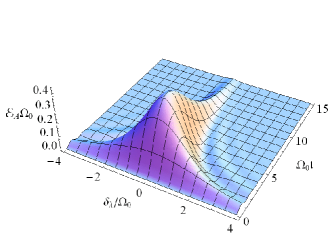
Figure 3: The density of entanglement $\mathcal{E}_{A}(\omega_{\lambda},t)$ between atom and bath is plotted for different times $t$ and reservoir mode frequencies $\omega_{\lambda}$. The coupling strength is: (a) $\Omega_{0}=10\Gamma$; and (b) $\Omega_{0}=0.1\Gamma$.

By examining the entanglement densities [Eqs. (17,18)] we can gain further insight into where the entanglement resides in this system and how it evolves over time. In Fig. 3 we show the atom-bath density of entanglement $\mathcal{E}_{A}(\omega_{\lambda},t)$ for both strong and weak couplings. The strong coupling case shows a complex behavior. First a central peak of entanglement appears in the vicinity of $\omega_{\lambda}\approx\omega_{0}$; note the peak at $\delta_{\lambda}\approx 0$ for short times in Fig. 3. The entanglement is then transferred to Rabi sidebands at $\delta_{\lambda}=\delta_{\pm}\approx\pm\Omega_{0}$. The sideband entanglement oscillations seen take place at half the frequency of the central peak entanglement oscillations. Ultimately all the entanglement decays at long times, $\mathcal{E}_{A}(\omega_{\lambda},t)\rightarrow 0$, as there can be no entanglement between bath and atom when the atomic population approaches zero. At that point the entanglement indicated by the concurrence in Fig. 2 must reside in reservoir mode entanglement which is examined in the next section, Sec. V.2. Fig. 3 shows that as Rabi sidebands develop in the reservoir excitation, the atom-bath entanglement moves from central frequencies to the sidebands at $\delta_{\lambda}=\delta_{\pm}$. The period doubling of the central peak is due to the oscillations of the excitation there, combined with the oscillations of atomic population. The population of the sideband modes is more stable, but oscillations of the atomic population result in oscillations of entanglement there, too.

For weak coupling, Fig. 3, the entanglement briefly resides across the whole reservoir structure. This is essentially because the coupling of the atom is over this same range. In weak coupling, however, Rabi sidebands do not develop. Instead the final population of bath modes will be over a relatively narrow frequency range well within the model Lorentzian profile, Eq. (30). Since both atomic, and mode population is needed for atom-bath entanglement, the narrow central frequency region is entangled only for a short while and then decays.

V.2 Entanglement between reservoir modes

As already mentioned, coupling the atom and the reservoir modes will induce an indirect coupling between the reservoir modes. Because of this, the modes will entangle and it is important to consider the properties of the mode-mode density of entanglement $\mathcal{E}_{R}$. In the long time limit one can easily obtain analytic expressions for the spectrum of excitation in the reservoir and from that calculate the density of entanglement for $t\rightarrow\infty$. Using the definition for the spectrum of reservoir excitation Eq. (19) with the solution (34) and Eq. (27), we find that for $t=\infty$

$$\begin{split}S(\omega_{\lambda},\infty)&=\frac{\Omega^{2}_{0}D(\omega_{\lambda})}{2\pi}\,\cdot\,\frac{\delta^{2}_{\lambda}+(\Gamma/2)^{2}}{(\delta^{2}_{\lambda}-\Omega^{2}_{0})^{2}+(\Gamma/2)^{2}\delta^{2}_{\lambda}}\\ \\ &=\frac{\Omega^{2}_{0}\Gamma/2}{\pi[(\delta_{\lambda}^{2}-\Omega_{0}^{2})^{2}+(\Gamma/2)^{2}\delta_{\lambda}^{2}]},\end{split}$$ (36)

where, as before, $\delta_{\lambda}=\omega_{\lambda}-\omega_{0}$ [Eq. (28)]. Taking Eq. (36) together with Eq. (21) it is straightforward to calculate the mode-mode density of entanglement for $t\rightarrow\infty$

$$\begin{split}&\mathcal{E}_{R}(\omega_{\lambda},\omega_{\mu},\infty)=\\ \\ &\frac{\Omega^{4}_{0}\Gamma^{2}}{2\pi^{2}\left[(\delta^{2}_{\lambda}-\Omega^{2}_{0})^{2}+(\Gamma/2)^{2}\delta^{2}_{\lambda}\right]\left[(\delta^{2}_{\mu}-\Omega^{2}_{0})^{2}+(\Gamma/2)^{2}\delta^{2}_{\mu}\right]}.\end{split}$$ (37)

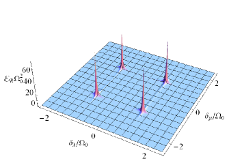
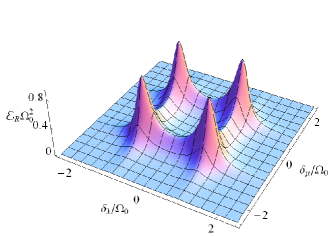
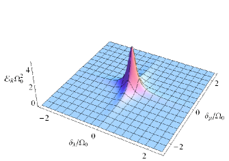
Figure 4: The density of entanglement $\mathcal{E}_{R}(\omega_{\lambda},\omega_{\mu},t)$ between bath modes for $t\rightarrow\infty$. The coupling strength is: (a) $\Omega_{0}=10\Gamma$; (b) $\Omega_{0}=\Gamma$; and (c) $\Omega_{0}=0.1\Gamma$.

Figure 4 shows the mode-mode density of entanglement for several couplings and in the limit $t\rightarrow\infty$. In the strong coupling case, Fig. 4, we see the formation of four sharp peaks which signify the existence of strong entanglement between the two symmetric modes $\delta_{\pm}$ as a result of the Rabi splitting. This picture has a simple and rather intuitive interpretation: the final state for the reservoir has the form of a Bell-like state between the two symmetric modes $\delta_{\pm}\approx\pm\Omega_{0}$. First we note that the final state takes the approximate form

$$|\psi(\infty)\rangle=|0\rangle_{a}\otimes\sum_{\lambda=1}^{N}\left(P_{+}(\omega_{\lambda})+P_{-}(\omega_{\lambda})\right)|\psi_{\lambda}\rangle.$$ (38)

where the two probability distributions $|P_{\pm}(\omega_{\lambda})|^{2}$ are centered at $\delta_{\lambda}=\delta_{+}$ and $\delta_{-}$ respectively. For $\Omega_{0}\gg\Gamma$, i.e. in the strong coupling regime, their width is very small which practically means that only the two modes $\delta_{\pm}$ are excited and, for this, the reservoir state can be approximately described by a Bell state of the form

$$|\psi(\infty)\rangle\approx|0\rangle_{a}\otimes|0_{\omega\neq\omega_{0}+\delta_{\pm}}\rangle\otimes\left(|1_{+}0_{-}\rangle+e^{\textrm{i}\phi}|0_{+}1_{-}\rangle\right)/\sqrt{2},$$ (39)

where $\phi$ is an arbitrary phase factor. This picture applies only at long times. For short times the mode-mode density of entanglement will initially have a distribution that peaks in the vicinity of $\omega_{\lambda}\approx\omega_{\mu}\approx\omega_{0}$. As time evolves this distribution breaks into four symmetrical peaks seen in Fig. 4, as a result of the Rabi splitting.

For moderate and weaker couplings, $\Omega_{0}=\Gamma$ and $\Omega_{0}\ll\Gamma$, the simple patterns observed in Fig. 4 for the mode-mode density of entanglement due to the Rabi splitting disappear. For example in Fig. 4 the density of entanglement for $t\rightarrow\infty$ and $\Omega_{0}=\Gamma$ is plotted. From this we can see that, for moderate couplings, although the distribution peaks around $\delta_{\mu}=\delta_{\lambda}=\delta_{\pm}$, the entanglement spreads over a wider range of reservoir frequencies. For even weaker couplings, Fig. 4, only modes in the vicinity of $\omega_{\lambda}\approx\omega_{0}$ are excited and thus the entanglement is created only between modes in this frequency range. This is the reason for having a peaked entanglement distribution with a centre at $\omega_{\mu}=\omega_{\lambda}=\omega_{0}$.

VI Conclusion

In this work we have presented a method for studying entanglement between a two-level atom and a large reservoir of modes such as may be found in, for example, a lossy cavity field. Our aim was to study entanglement between the atom and the reservoir, and within the reservoir itself. To do this we restricted our interest to a simple case where the reservoir modes can be treated as qubits. Using global entanglement, we derived the entanglement densities $\mathcal{E}_{A}$ and $\mathcal{E}_{R}$ for the reservoir modes. These distributions have been given in terms of the well known two-qubit concurrences, and can be calculated from the reservoir excitation spectrum. The entanglement densities are then used both for studying entanglement between the atom and the reservoir modes, and also between the modes.

In considering different dynamical regimes defined in terms of the coupling strength, we noticed that when strong interactions occur, the reservoir modes are entangled in a “Bell-like” state in the long time limit. This long time limit is a regime where no excitation remains in the atom and all the entanglement is amongst the reservoir modes. Since there is no direct interaction between the bath-modes, see the Hamiltonian (22), the final entanglement arises through indirect interaction. Another way of viewing this is that in the strong coupling regime we have a non-Markovian system. In such a case, as the atom decays, some information resides in part of the reservoir in a way that it can be returned to the atom later Mazzola09a . This allows the indirect coupling between the reservoir modes which creates the entanglement. In the weak coupling (Markovian) case, the information does not return to the atomic system and the reservoir entanglement cannot be created.

In the transition from strong to weak coupling, the “Bell-like” state of Fig. 4 coalesces into a single peaked structure as was seen in Fig. 4. Based on the interpretation given above we would expect that the transition to a single peak takes place as the system becomes Markovian rather than non-Markovian. In principle this could be tested with a measure of non-Markovianity Breuer09 .

In conclusion, when considering entanglement between an atom and a large reservoir, the analysis can be formulated in terms of entanglement density functions. These distributions can be associated with the spectrum of reservoir excitation, a quantity that can be measured, for example, in cavity QED experiments. Although the model considered here, an atom coupled to a Lorentzian reservoir, is rather simple, it can be extended to consider more complicated reservoir structures such as model photonic band gaps. Potentially, one could consider generalizations for the density of entanglement, and also extend the model beyond the assumption of a single excitation in the system.

Appendix A Global entanglement

For the completeness of our analysis, we show here how the global entanglement for the pure state $|\psi(t)\rangle$, Eq. (1), can be derived. First, the state $|\psi(t)\rangle$ can be written as a pure state of $N+1$ qubits, i.e.

$$|\psi(t)\rangle=c_{0}|{\bf{0}}\rangle+\sum_{j}c_{j}(t)|\psi_{j}\rangle,$$ (40)

where $j=a$ for the atom, or $j=\lambda=1,\cdots,N$ for the reservoir modes. The vacuum state $|{\bf{0}}\rangle$ is given in Eq. (2), while $|\psi_{j}\rangle=|\psi_{a}\rangle$ [Eq. (3)] for $j=a$, or is given by Eq. (4) if $j=\lambda$, i.e. refers to a reservoir mode.

Next we calculate the reduced two-qubit density matrix $\rho_{ji}$

$$\rho_{ji}=\textrm{tr}_{k\neq j,i}\{\rho\}=\langle\chi_{0}|\rho|\chi_{0}\rangle+\sum_{k\neq j,i}\langle\chi_{k}|\rho|\chi_{k}\rangle,$$ (41)

where $|\chi_{0}\rangle$ is the $N-2$-qubit vacuum state

$$|\chi_{0}\rangle=\prod_{k\neq i,j}|0_{k}\rangle,$$ (42)

and $|\chi_{k}\rangle$ is the $N-2$-qubit state with a single excitation, i.e.

$$|\chi_{k}\rangle=|0\cdots 01_{k}0\cdots 0\rangle.$$ (43)

With these definitions for $|\chi_{0}\rangle$ and $|\chi_{k}\rangle$, the reduced density matrix takes the form

$$\rho_{ji}=\left(\begin{array}[]{cccc}1-|c_{j}|^{2}-|c_{i}|^{2}&c^{\ast}_{0}c_{i}&c^{\ast}_{0}c_{j}&0\\ c_{0}c^{\ast}_{i}&|c_{i}|^{2}&c_{j}c^{\ast}_{i}&0\\ c_{0}c^{\ast}_{j}&c^{\ast}_{j}c_{i}&|c_{j}|^{2}&0\\ 0&0&0&0\end{array}\right),$$ (44)

where the basis states, starting from top and moving to bottom, are

$$|0_{j}0_{i}\rangle,\quad|0_{j}1_{i}\rangle,\quad|1_{j}0_{i}\rangle,\quad|1_{j}1_{i}\rangle.$$ (45)

The concurrence $c(\rho_{ji})$, Eq. (13), for this density matrix reads

$$c^{2}(\rho_{ji})=4|c_{j}|^{2}|c_{i}|^{2}.$$ (46)

In order to calculate the global entanglement, we derive the single qubit density matrix from Eq. (44) by tracing out the $i$-qubit

$$\rho_{j}=\left(\begin{array}[]{cc}1-|c_{j}|^{2}&c_{0}c^{\ast}_{j}\\ c^{\ast}_{0}c_{j}&|c_{j}|^{2}\end{array}\right),$$ (47)

where the basis states are $|0_{j}\rangle$ and $|1_{j}\rangle$. Using this we first calculate $\rho^{2}_{j}$ and then its trace

$$\textrm{tr}\rho^{2}_{j}=1+2|c_{j}|^{2}\left(|c_{j}|^{2}+|c_{0}|^{2}-1\right),$$ (48)

which after using probability conservation becomes

$$\textrm{tr}\rho^{2}_{j}=1-2|c_{j}|^{2}\sum_{i\neq j}|c_{i}|^{2}.$$ (49)

Substituting in Eq. (5) for the global entanglement we have

$$Q(|\psi\rangle)=\frac{2}{N+1}\sum_{j}\sum_{i\neq j}2|c_{j}|^{2}|c_{i}|^{2}.$$ (50)

Separating the atom-mode terms and the mode-mode terms, and taking into account the symmetry of the two-qubit concurrence

$$c^{2}(\rho_{ji})=c^{2}(\rho_{ij}),$$ (51)

it takes the form

$$Q(|\psi\rangle)=\frac{2}{N+1}\left(\sum_{\lambda=1}^{N}c^{2}(\rho_{a\lambda})+\sum_{1\leq\lambda<\mu\leq N}c^{2}(\rho_{\lambda\mu})\right),$$ (52)

which leads to the result of Eqs. (9) and (10).

References

- (1) L. Amico, R. Fazio, A. Osterloh, and V. Vedral, Rev. Mod. Phys. 80, 517 (2008)
- (2) R. Horodecki, P. Horodecki, M. Horodecki, and K. Horodecki, Rev. Mod. Phys. 81, 865 (2009)
- (3) M. A. Nielsen and I. L. Chuang, Quantum computation and quantum information (Cambridge University Press, Cambridge, 2000)
- (4) D. Leibfried, R. Blatt, C. Monroe, and D. Wineland, Rev. Mod. Phys. 75, 281 (2003)
- (5) F. Dalfovo, S. Giorgini, L. P. Pitaevskii, and S. Stringari, Rev. Mod. Phys. 71, 463 (1999)
- (6) A. J. Leggett, Rev. Mod. Phys. 73, 307 (2001)
- (7) J. M. Raimond, M. Brune, and S. Haroche, Rev. Mod. Phys. 73, 565 (2001)
- (8) B. T. H. Varcoe, S. Brattke, and H. Walther, New J. Phys. 6, 97 (2004)
- (9) P. Lambropoulos, G. M. Nikolopoulos, T. R. Nielsen, and S. Bay, Rep. Prog. Phys. 63, 455 (2000)
- (10) G. M. Nikolopoulos, P. Lambropoulos, and N. P. Proukakis, J. Phys. B: At. Mol. Opt. Phys. 36, 2797 (2003)
- (11) C. Lazarou, G. M. Nikolopoulos, and P. Lambropoulos, J. Phys. B: At. Mol. Opt. Phys. 40, 2511 (2007)
- (12) G. M. Nikolopoulos, C. Lazarou, and P. Lambropoulos, J. Phys. B: At. Mol. Opt. Phys. 41, 025301 (2008)
- (13) N. I. Cummings and B. L. Hu, Phys. Rev. A 77, 053823 (2008)
- (14) S. Haroche and J. M. Raimond, Exploring the quantum (Oxford University Press, New York, 2006)
- (15) H. P. Breuer and F. Petruccione, The theory of open quantum systems (Oxford University Press, New York, 2002)
- (16) B. M. Garraway, Phys. Rev. A 55, 2290 (1997)
- (17) B. M. Garraway, Phys. Rev. A 55, 4636 (1997)
- (18) S. Hill and W. K. Wootters, Phys. Rev. Lett. 78, 5022 (1997)
- (19) W. K. Wootters, Phys. Rev. Lett. 80, 2245 (1998)
- (20) F. Mintert, A. R. Carvalho, M. Kus, and A. Buchleitner, Phys. Rep. 415, 207 (2005)
- (21) H. Barnum, E. Knill, G. Ortiz, R. Somma, and L. Viola, Phys. Rev. Lett. 92, 107902 (2004)
- (22) D. A. Meyer and N. R. Wallach, J. Math. Phys. 43, 4273 (2002)
- (23) S. J. Akhtarshenas, J. Phys. A: Math. Gen. 38, 6777 (2005)
- (24) B. Bellomo, R. Lo Franco, and G. Compagno, Phys. Rev. Lett. 99, 160502 (2007)
- (25) B. Bellomo, R. Lo Franco, S. Maniscalco, and G. Compagno, Phys. Rev. A 78, 060302 (2008)
- (26) S. Maniscalco, F. Francica, R. L. Zaffino, N. Lo Gullo, and F. Plastina, Phys. Rev. Lett. 100, 090503 (2008)
- (27) F.-Q. Wang, Z.-M. Zhang, and R.-S. Liang, Phys. Rev. A 78, 042320 (2008)
- (28) D. P. Fussell and M. M. Dignam, Phys. Rev. A 77, 053805 (2008)
- (29) I. Thanopulos, P. Brumer, and M. Shapiro, J. Chem. Phys. 129, 194104 (2008)
- (30) M. Al-Amri, G.-x. Li, R. Tan, and M. S. Zubairy, Phys. Rev. A 80, 022314 (2009)
- (31) Y. Li, J. Zhou, and H. Guo, Phys. Rev. A 79, 012309 (2009)
- (32) L. Mazzola, S. Maniscalco, J. Piilo, K.-A. Suominen, and B. M. Garraway, Phys. Rev. A 80, 012104 (Jul 2009)
- (33) L. Mazzola, S. Maniscalco, J. Piilo, and K.-A. Suominen, J. Phys. B: At., Mol. Opt. Phys. 43, 085505 (2010)
- (34) J. Zhou, C. Wu, M. Zhu, and H. Guo, J. Phys. B: At. Mol. Optic. Phys. 42, 215505 (2009)
- (35) E. Ferraro, M. Scala, R. Migliore, and A. Napoli, Phys. Rev. A 80, 042112 (2009)
- (36) F. Francica, S. Maniscalco, J. Piilo, F. Plastina, and K.-A. Suominen, Phys. Rev. A 79, 032310 (2009)
- (37) X. Xiao, M.-F. Fang, Y.-L. Li, K. Zeng, and C. Wu, J. Phys. B: At. Mol. Opt. Phys. 42, 235502 (2009)
- (38) Y. J. Zhang, Z. X. Man, and Y. J. Xia, Eur. Phys. J. D 55, 173 (2009)
- (39) L. Mazzola, S. Maniscalco, K. Suominen, and B. Garraway, Quantum Inf. Process. 8, 577 (2009)
- (40) L. Mazzola, S. Maniscalco, J. Piilo, K.-A. Suominen, and B. M. Garraway, Phys. Rev. A 79, 042302 (2009)
- (41) Z. He, J. Zou, B. Shao, and S.-Y. Kong, J. Phys. B: At. Mol. Opt. Phys. 43, 115503 (2010)
- (42) Y.-J. Zhang, Z.-X. Man, X.-B. Zou, Y.-J. Xia, and G.-C. Guo, J. Phys. B: At. Mol. Opt. Phys. 43, 045502 (2010)
- (43) Z. X. Man, Y. J. Zhang, F. Su, and Y. J. Xia, Eur. Phys. J. D 58, 147 (2010)
- (44) Z. X. Man, Y. J. Zhang, F. Su, and Y. J. Xia, Eur. Phys. J. D 58, 147 (2010)
- (45) Y. J. Zhang, Z. X. Man, Y. J. Xia, and G. C. Guo, Eur. Phys. J. D 58, 397—401 (2010)
- (46) Q.-J. Tong, J.-H. An, H.-G. Luo, and C. H. Oh, Phys. Rev. A 81, 052330 (2010)
- (47) L. Mazzola, B. Bellomo, R. Lo Franco, and G. Compagno, Phys. Rev. A 81, 052116 (2010)
- (48) Q.-J. Tong, J.-H. An, H.-G. Luo, and C. H. Oh, Phys. Rev. A 81, 052330 (2010)
- (49) B. Wang, Z.-Y. Xu, Z.-Q. Chen, and M. Feng, Phys. Rev. A 81, 014101 (2010)
- (50) Q.-J. Tong, J.-H. An, H.-G. Luo, and C. H. Oh, J. Phys. B: At. Mol. Opt. Phys. 43, 155501 (2010)
- (51) F. F. Fanchini, T. Werlang, C. A. Brasil, L. G. E. Arruda, and A. O. Caldeira, Phys. Rev. A 81, 052107 (2010)
- (52) A. Hamadou-Ibrahim, A. R. Plastino, and C. Zander, J. Phys. A: Math. Theor. 43, 055305 (2010)
- (53) J.-G. Li, J. Zou, and B. Shao, Phys. Rev. A 81, 062124 (2010)
- (54) Z. Y. Xu, W. L. Yang, and M. Feng, Phys. Rev. A 81, 044105 (2010)
- (55) I. E. Linington and B. M. Garraway, J. Phys. B: At. Mol. Opt. Phys. 39, 3383 (2006)
- (56) S. John and T. Quang, Phys. Rev. A 50, 1764 (1994)
- (57) A. G. Kofman, G. Kurizki, and B. Sherman, J. Mod. Opt. 41, 353 (1994)
- (58) B. J. Dalton, S. M. Barnett, and B. M. Garraway, Phys. Rev. A 64, 053813 (2001)
- (59) H.-P. Breuer, E.-M. Laine, and J. Piilo, Phys. Rev. Lett. 103, 210401 (Nov 2009)