Anomalous criticality in the quantum Hall transition at $n=0$ Landau level of graphene
with chiral-symmetric disorders

Abstract

We investigate numerically whether the chiral symmetry is the sole factor dominating the criticality of the quantum Hall transitions in disordered graphene. When the disorder respects the chiral symmetry, the plateau-to-plateau transition at the $n=0$ Landau level is shown to become anomalous (i.e., step-function-like). Surprisingly, however, the anomaly is robust against the inclusion of the uniform next-nearest neighbor hopping, which degrades the chiral symmetry of the lattice models. We have also shown that the ac (optical) Hall conductivity exhibits a robust plateau structure when the disorder respects the chiral symmetry.

I Introduction

Kicked off by the recent observation of the characteristic quantum Hall effect in graphene,Geim ; Kim ; ZhengAndo the effect of disorder has attracted considerable attention.KA ; SM ; OGM ; KHA A key interest that is specific to the electronic structure of graphene is the chiral (A-B sub-lattice) symmetry HFA ; HChiral and the scattering between two Dirac cones that reside at K and K’ points in k-space. Accordingly, the nature of disorder (i.e., whether the disorder preserves the chiral symmetry or not) should be essential in discussing the electronic properties of disordered graphene. A potential disorder breaks the chiral symmetry, whereas a disorder in bonds preserves the symmetry. The spatial range of disorder is another important factor, since the inter-valley scattering occurs when the disorder is short-ranged while strongly suppressed when long-ranged.

In our previous papers KHA , we have considered the disorder in the hopping energies as a model for a ripple,Meyer ; GLERSRLM which is an intrinsic disorder in graphene. We have clearly demonstrated that for such a chiral-symmetry preserving disorder, the criticality of the quantum Hall transition at the $n=0$ Landau level becomes anomalously sensitive to the spatial correlation of disorder: When the spatial range of the bond disorder exceeds a few lattice constant, no broadening of the graphene-specific $n=0$ Landau level occurs and the associated step-function like Hall transition exhibits an anomalous (almost fixed-point) criticality. This sharply contrasts with the case of potential disorder which degrades the chiral symmetry, where the criticality is similar to the ordinary quantum Hall transition.NRKMF

Now, when one describes the actual graphene with a tight-binding model, the effect of the next-nearest neighbor hopping in the honeycomb lattice is not negligible.Neto ; Reich ; Nakajima Since the next-nearest neighbor hopping $t^{\prime}$ connects sites in the same sub-lattice, the chiral symmetry of the original the honeycomb lattice is broken, so that one might naively think that the speciality about the $n=0$ Landau level associated with the chiral symmetry should be washed away. It is to be noted, however, that the space group (i.e., rotation and reflection symmetries as well as the translation symmetry) of the honeycomb lattice are preserved, and, indeed, the two Dirac cones still exist at $K$ and $K^{\prime}$ points at an energy shifted from zero.SW The existence of the doubled Dirac cones has a topological origin. For instance, they exist even in the presence of a third-neighbor hopping $t^{\prime\prime}$ in one of the three directions (which is equivalent to the $\pi$ flux model) with $t^{\prime}=0$ as shown in Ref. HFA, , where the lattice continuously crosses over to the square lattice as $t^{\prime\prime}$ is increased. In such a system, the Dirac cones are located at general points away from K and K’ in the Brillouin zone. If we add $t^{\prime}$ in this case, tilted Dirac cones appear at a non-zero energy. The tilted Dirac cones are interesting, since they have been observed in an organic system $\alpha$-(BEDT-TTF)₂I₃ under a high pressure.KKS ; TSTNK

Given these variety of situations, we want to clarify in the present paper whether the anomalous criticality is preserved or washed out. First, we shall clarify the question: Do we have to discriminate the presence or otherwise of the chiral symmetry in the underlying honeycomb lattice (before we turn on the disorder) and the presence or otherwise of the chiral symmetry in the disorder? In order to study these, we adopt the honeycomb lattice model rather than the effective Dirac model, since the chiral symmetry has to do with the AB sublattices. To examine the robustness of the criticality for the $n=0$ Landau level, we calculate the Hall conductivity in the honeycomb lattice as well as the $\pi$ flux model with the bond disorder to examine the influence of the next-nearest neighbor hopping. We find that the anomalous criticality at the $n=0$ Landau level for the long-ranged bond disorder is robust against the inclusion of the uniform next-nearest neighbor hopping, namely the break down of the chiral symmetry of the lattice models, which yields, in general, the energy shift as well as the tilt of the Dirac cones. The Hall conductivity for non-interacting electron systems is mathematically equivalent to a topological integer called a Chern number. TKNN ; NTW ; Hedge ; AokiAndo Taking into account the recent progress in numerical evaluation of the Chern number, HC ; FHS ; HFS we adopt a formulation based on the lattice gauge technique to evaluate the Hall conductivity in disordered finite systems. The formulation is based on the topological invariant used in the lattice gauge theory, which can also be understood as a two dimensional generalization of the King-Smith-Vanderbilt formula for polarization.FHS ; KSV The present formulation has been successfully applied to the calculation of the Hall conductivity not only for uniform systems but also for disordered systems.SMH

Our second question is: How the criticality appears in the ac (optical) Hall conductivity, $\sigma_{xy}(\omega)$? The optical response of QHE system is now attracted growing interest. For instance, the cyclotron emission from graphene QHE system has been studied theoretically morimoto-CE as well as experimentally with infrared transmission.sadowski06 Specifically, Morimoto et almorimoto-opthall have shown that the optical Hall conductivity $\sigma_{xy}(\omega)$ has a Hall plateau structure even in the ac ($\sim$ THz) regime, both in the ordinary two-dimensional electron gas (2DEG) and in graphene in the quantum Hall regime, although the plateau height is no longer quantized in ac. In graphene $\sigma_{xy}(\omega)$, which reflects the unusual Landau level structure, the plateau structure remains against a significant strength of disorder due to an effect of localization. For 2DEG the THz spectroscopy has recently been performed, and a plateau structure of optical Hall conductivity has been detected in the THz region.ikebe-THz10 Hence it is interesting to investigate the consequence of the chiral symmetry in the ac Hall effect in graphene.

II Chiral symmetry in lattice models

Let us begin with the chiral symmetry. The symmetry is defined by the existence of a local operator $\gamma$ with $\gamma^{2}=1$ that anti-commutes with the Hamiltonian $H$ as $\{\gamma,H\}=0$. For bipartite lattices such as honeycomb and square, the lattice can be decomposed into $A$ and $B$ sub-lattices. If we take $\gamma=\prod_{i\in A}\exp({\rm i}\pi c_{i}^{\dagger}c_{i})$, the fermion operator $c_{i}$ is transformed as $\gamma c_{i}\gamma=-c_{i}$ for $i\in A$ and $\gamma c_{i}\gamma=c_{i}$ for $i\in B$. We can readily show that the lattice model that has only hopping terms $t_{ij}c_{i}^{\dagger}c_{j}$ connecting A and B sites has the chiral symmetry $\{\gamma,H\}=0$, irrespective of the details of the hopping terms $t_{ij}$.

An important consequence of the chiral symmetry is that the energy levels appear in pairs, $\{E,-E\}$, and hence the energy spectrum is symmetric around $E=0$. Assume that $\psi_{E}$ is an eigenstate with energy $E$ satisfying $H\psi_{E}=E\psi_{E}$. Then the state $\gamma\psi_{E}$ is an eigenstate with energy $-E$, since $H(\gamma\psi_{E})=-\gamma H\psi_{E}=-E(\gamma\psi_{E})$. For $E=0$ the eigenstates $\psi_{E=0}$ and $\gamma\psi_{E=0}$ are degenerated. We can rearrange the eigenstates into $\psi_{\pm}=(1\pm\gamma)\psi_{E=0}$ to make them simultaneous eigenstates of $\gamma$ with $\gamma\psi_{\pm}=\pm\psi_{\pm}$. This implies that the system has an additional symmetry in the zero-energy space. From the definition of $\gamma$, it is clear that the eigenstate $\psi_{+(-)}$ has its amplitudes only on the $B(A)$ sub-lattice sites. The criticality of the Hall transition at $E=0$ can thus be sensitive to the presence or absence of the chiral symmetry.AZ

III DC Hall conductivity

III.1 Hamiltonian

The tight-binding Hamiltonian for the honeycomb lattice with the next-nearest neighbor hopping is given by

$$H=\sum_{\langle i,j\rangle}^{\rm nn}t_{ij}e^{-2\pi{\rm i}\theta_{ij}}c_{i}^{\dagger}c_{j}+\sum_{\langle i,j\rangle}^{\rm nnn}t^{\prime}e^{-2\pi{\rm i}\theta^{\prime}_{ij}}c_{i}^{\dagger}c_{j}+{\rm h.c.},$$

where the summation is performed for nearest neighbor sites in the first term and for next-nearest neighbor sites in the second term (Fig. 1). Here $t_{ij}$ and $t^{\prime}$ are assumed to be real, while the Peierls phases, $\{\theta_{ij}\}$ and $\{\theta^{\prime}_{ij}\}$, are determined such that the sum of the phases around a loop is equal to the magnetic flux piercing the loop in units of the flux quantum $\phi_{0}=h/e$. We specify the strength of the uniform magnetic field by the magnetic flux $\phi$ per hexagon in the honeycomb lattice. We introduce a bond randomness in the nearest-neighbor transfer energy as $t_{ij}=-t+\delta t_{ij}$, where $t$ and $\delta t_{ij}$ denote the uniform and the disordered components, respectively. The disorder in $\delta t_{ij}$ is assumed to have a Gaussian distribution $P(\delta t)=e^{-\delta t^{2}/2\sigma^{2}}/{\sqrt{2\pi\sigma^{2}}}$ with a variance $\sigma$. The spatial correlation length $\eta$ in the random components is specified by requiring

$$\langle\delta t_{ij}\delta t_{kl}\rangle=\langle\delta t^{2}\rangle e^{-|\mbox{\boldmath$r$}_{ij}-\mbox{\boldmath$r$}_{kl}|^{2}/4\eta^{2}},$$

where $\mbox{\boldmath$r$}_{ij}$ represents the bond $t_{ij}$, and $\langle\rangle$ the ensemble averageKawa . The length is hereafter measured in units of the distance $a$ between nearest-neighbor sites. It is to be noted that the Hamiltonian $H$ is chiral symmetric if $t^{\prime}=0$ even in the presence of disorder in the nearest neighbor hopping $t_{ij}$, while the chiral symmetry is broken for $t^{\prime}\neq 0$. In actual graphene, the magnitude of $t^{\prime}$ is estimated to be $0.2\sim 0.02t$.Reich

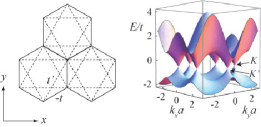
Figure 1: Left: Honeycomb lattice with nearest neighbor hopping $-t$ (solid lines) and next-nearest neighbor hopping $t^{\prime}$ (dotted lines). Right: Energy dispersion for $\phi=0,t^{\prime}/t=0.15$. Dirac cones are located at $K=(2\pi/3\sqrt{3}a,2\pi/3a)$ and $K^{\prime}=(4\pi/3\sqrt{3}a,0)$ with energy $-3t^{\prime}$.Neto

III.2 Hall conductivity as a Chern number

In order to evaluate the Hall conductivity, let us consider a $L_{x}\times L_{y}$ system, and impose boundary conditions for the single-particle wave function $|\varphi\rangle$ as $T_{x(y)}(L_{x(y)})|\varphi\rangle=e^{{\rm i}\phi_{x(y)}}|\varphi\rangle,$ where $T_{x(y)}(L_{x(y)})$ denotes the single-particle magnetic translation operator in the $x(y)$ direction. The string gauge in the corresponding brick-layer lattice is adopted to treat this twisted boundary conditions. HIM When the energy gap exists above the Fermi energy $E_{F}$, the Hall conductivity $\sigma_{xy}$ can related to a topological integer $C_{E}$ called the Chern number as HFA ; TKNN ; NTW ; Hedge ; AokiAndo ; HIM $\sigma_{xy}=-\frac{e^{2}}{h}C_{E}$ with

$$C_{E}=\frac{1}{2\pi{\rm i}}\int_{T^{2}}d^{2}\mbox{\boldmath$\phi$}(\partial_{\phi_{x}}\langle\psi|\partial_{\phi_{y}}\psi\rangle-\partial_{\phi_{y}}\langle\psi|\partial_{\phi_{x}}\psi\rangle),$$

where $\psi$ denotes the wave function of the Fermi sea in the twisted boundary conditions specified by the phase $\mbox{\boldmath$\phi$}=(\phi_{x},\phi_{y}),(0\leq\phi_{x(y)}\leq 2\pi)$ with the normalization $\langle\psi|\psi\rangle=1$ and $T^{2}$ is the two-dimensional parameter space for the phase $\phi$. The Chern number can be expressed, by introducing a $\delta\phi_{x}$ by $\delta\phi_{y}$ mesh for the parameter space $T^{2}$, as $C_{E}=\frac{1}{2\pi{\rm i}}\sum_{m,n}F_{m,n}$ with

$$F_{m,n}=\oint_{\partial S_{mn}}\mbox{\boldmath$A$}\cdot d\mbox{\boldmath$\phi$},\quad\mbox{\boldmath$A$}=\langle\psi|\nabla_{\phi}\psi\rangle.$$

Here $S_{mn}$ stands for a $\delta\phi_{x}$ by $\delta\phi_{y}$ square of the mesh with points $\mbox{\boldmath$\phi$}=(m\delta\phi_{x},n\delta\phi_{y}),((m+1)\delta\phi_{x},n\delta\phi_{y}),((m+1)\delta\phi_{x},(n+1)\delta\phi_{y}),(m\delta\phi_{x},(n+1)\delta\phi_{y})$. The surface integral on $S_{mn}$ is replaced by the line integral by Stokes’ theorem. It is useful to note that this line integral $F_{m,n}$ can be written as

$$F_{m,n}=\ln U_{x}(\mbox{\boldmath$\phi$})U_{y}(\mbox{\boldmath$\phi$}+\mbox{\boldmath$\Delta\phi$}_{x})U_{x}^{-1}(\mbox{\boldmath$\phi$}+\mbox{\boldmath$\Delta\phi$}_{y})U_{y}^{-1}(\mbox{\boldmath$\phi$}),$$

with $U_{\alpha}(\mbox{\boldmath$\phi$})=\exp(\int_{\mbox{\boldmath$\phi$}}^{\mbox{\boldmath$\phi$}+\mbox{\boldmath$\Delta\phi$}_{\alpha}}A_{\alpha}d\phi_{\alpha})\quad(\alpha=x,y),$ where $\mbox{\boldmath$\Delta\phi$}_{x}=(\delta\phi_{x},0)$, $\mbox{\boldmath$\Delta\phi$}_{y}=(0,\delta\phi_{y})$ and $\mbox{\boldmath$\phi$}=(m\delta\phi_{x},n\delta\phi_{y})$.

Following Fukui et al.,FHS we consider a link variable defined on the mesh as

$$\tilde{U}_{\alpha}(\mbox{\boldmath$\phi$})=\frac{\langle\psi(\mbox{\boldmath$\phi$})|\psi(\mbox{\boldmath$\phi$}+\mbox{\boldmath$\Delta\phi$}_{\alpha})\rangle}{|\langle\psi(\mbox{\boldmath$\phi$})|\psi(\mbox{\boldmath$\phi$}+\mbox{\boldmath$\Delta\phi$}_{\alpha})\rangle|},\quad(\alpha=x,y),$$

and define the Chern number $\tilde{C}_{E}$ on the mesh as $\tilde{C}_{E}=\frac{1}{2\pi{\rm i}}\sum_{m,n}\tilde{F}_{m,n},$ where

$$\tilde{F}_{m,n}=\ln\tilde{U}_{x}(\mbox{\boldmath$\phi$})\tilde{U}_{y}(\mbox{\boldmath$\phi$}+\mbox{\boldmath$\Delta\phi$}_{x})\tilde{U}_{x}^{-1}(\mbox{\boldmath$\phi$}+\mbox{\boldmath$\Delta\phi$}_{y})\tilde{U}_{y}^{-1}(\mbox{\boldmath$\phi$})$$

with $-\pi<\tilde{F}_{m,n}/{\rm i}\leq\pi$. The Chern number $\tilde{C}_{E}$ defined in such a way on the mesh reduces to the Chern number $C_{E}$ defined on the continuum space in the limit $\delta\phi_{x(y)}\rightarrow 0$. It is to be noted that $\tilde{C}_{E}$ is gauge invariant, and takes an integer value for an arbitrary mesh width $\delta\phi_{x(y)}$. We have then $\tilde{C}_{E}=C_{E}$ for a fine enough mesh. FHS ; HFS

In the present case, the wave function of the Fermi sea $|\psi\rangle$ is a Slater determinant of the single-particle wave function $|\varphi\rangle$, so that the link variable $\tilde{U}_{\alpha}(\mbox{\boldmath$\phi$})$ for an $M$ particle state is given by HC $\tilde{U}_{\alpha}(\mbox{\boldmath$\phi$})={\det V_{\alpha}(\mbox{\boldmath$\phi$})}/{|\det V_{\alpha}(\mbox{\boldmath$\phi$})|},$ where $V_{\alpha}(\mbox{\boldmath$\phi$})$ is an $M\times M$ matrix. The elements of $V$ are defined by $(V_{\alpha}(\mbox{\boldmath$\phi$}))_{ij}=\langle\varphi_{i}(\mbox{\boldmath$\phi$})|\varphi_{j}(\mbox{\boldmath$\phi$}+\mbox{\boldmath$\Delta\phi$}_{\alpha})\rangle,\ (1\leq i,j\leq M)),$ with the $i$-th single-particle eigenstate $|\varphi_{i}(\mbox{\boldmath$\phi$})\rangle$ satisfying $H|\varphi_{i}(\mbox{\boldmath$\phi$})\rangle=\varepsilon_{i}|\varphi_{i}(\mbox{\boldmath$\phi$})\rangle$ ($\varepsilon_{1}\leq\ldots\leq\varepsilon_{k}\leq\varepsilon_{k+1},\ldots$) in the boundary condition specified by $\phi$, where the Fermi energy $E_{F}$ is assumed to lie between $\varepsilon_{k}$ and $\varepsilon_{k+1}$. The energy gap at the Fermi energy is mostly guaranteed for finite and random systems due to the level repulsion. We thus adopt this formulation to evaluate the Chern numbers for each sample. By taking an average over samples in each energy bin, we obtain ensemble-averaged Hall conductivity as a function of the Fermi energy.

III.3 Anomalous criticality in the $n=0$ level

The Chern number $C_{E}$ for the case of a bond-disordered honeycomb lattice with $t^{\prime}=0$, where the chiral symmetry is exactly preserved, is shown in Fig.2. We can clearly see that the plateau transition in the $n=0$ Landau level at $E=0$ becomes almost step-function like as a function of the Fermi energy as soon as the spatial correlation length, $\eta$, of the bond disorder exceeds the lattice constant $a$, as previously shown in Ref. KHA, . Remarkably, this behavior is fixed-point like in that it shows almost no system-size dependence. The anomalous Hall transition is accompanied by the absence of broadening of the $n=0$ Landau level.

Next we show what happens when we switch on the next-nearest neighbor hopping $t^{\prime}\neq 0$. Note that the Dirac cones still exist at $K$ and $K^{\prime}$ at an energy, $-3t^{\prime}$, shifted from zero.Neto The Hall conductivity in the case of $t^{\prime}/t=0.05$ is shown in Fig. 3 for several values of the disorder correlation length $\eta$. It is clearly seen that the Hall plateau transition at the $n=0$ Landau level is again anomalously sensitive to the spatial correlation of the bond disorder. The results for different system sizes are displayed in Fig.4, where we see little size-dependence at $n=0$. This occurs despite the fact that the chiral symmetry of the lattice model is broken by the next-nearest neighbor hopping $t^{\prime}\neq 0$. Consequently, the energy spectrum is not symmetric about $E=0$ with the $n=0$ Landau level shifted from $E=0$. If we vary the strength of the next-nearest neighbor hopping $t^{\prime}$, the critical energy for the anomalous Hall transition associated with the $n=0$ Landau level is simply shifted with $t^{\prime}$ (Fig.5). For $n=\pm 1$ Landau levels, by contrast, the usual scaling behavior (i.e., a narrower transition region for a larger system) is observed (Fig. 4).

The present results amount to that the anomalous transition remains at the energy of the Dirac cones, where the breakdown of the usual chiral symmetry does not affect the anomalous criticality although the energy spectrum is affected. This stability of the anomalous criticality is attributed to the preserved effective chiral symmetry for the $2\times 2$ low-energy effective Hamiltonian in the vicinity of the Dirac cones.Neto

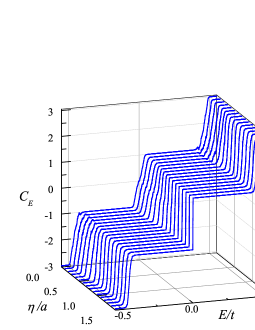
Figure 2: (Color online) The Chern number $C_{E}$ (Hall conductivity in units of $e^{2}/h)$ as a function of the Fermi energy $E/t$ for various values of the spatial correlation length $\eta/a$ of the bond disorder, for $t^{\prime}/t=0$, $\phi/\phi_{0}=1/50$, $\sigma/t=0.115$ and $L_{x}/(\sqrt{3}a/2)=L_{y}/(3a/2)=20$.

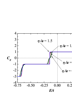
Figure 3: (Color online) The Chern number $C_{E}$ (Hall conductivity in units of $e^{2}/h)$ as a function of the Fermi energy $E/t$ in the presence of the next-nearest-neighbor hopping $t^{\prime}/t=0.05$ for $\eta/a=0.0,0.5,1.0$ and $1.5$, for $\phi/\phi_{0}=1/36$, $\sigma/t=0.115$ and $(L_{x}/(\sqrt{3}a/2),L_{y}/(3a/2))=(24,18)$.

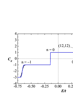
Figure 4: (Color online) The Chern number $C_{E}$ (Hall conductivity in units of $e^{2}/h)$ as a function of the Fermi energy $E/t$ in the presence of the next-nearest-neighbor hopping $t^{\prime}/t=0.05$ for $\eta/a=1.5$, for $\phi/\phi_{0}=1/36$, $\sigma/t=0.115$ and $(L_{x}/(\sqrt{3}a/2),L_{y}/(3a/2))=(24,18)$ and $(12,12)$.

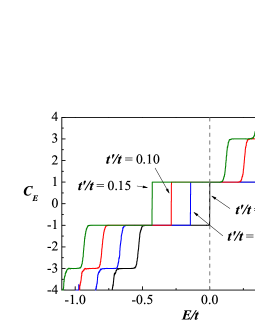
Figure 5: (Color online) The Chern nmber $C_{E}$ (Hall conductivity in units of $e^{2}/h)$ as a function of the Fermi energy $E/t$ for various values of the next-nearest-neighbor hopping $t^{\prime}$, with a fixed $\eta/a=1.5$, $\phi/\phi_{0}=1/36$, $\sigma/t=0.115$ and $(L_{x}/(\sqrt{3}a/2),L_{y}/(3a/2))=(24,18)$.

III.4 Tilted Dirac cones

To examine further the robustness of the anomaly at the $n=0$ Landau level, we consider a lattice model having an third-neighbor hopping $t^{\prime\prime}$ across the hexagon of the honeycomb lattice (Fig. 6). It has been shown HFA that, for the case of $t^{\prime}=0$, this model has also two Dirac cones in the first Brillouin zone for $-1<t"<3$, which are adiabatically connected to the Dirac cone in the original honeycomb lattice as the hopping $t"$ is continuously varied. When $t"$ is increased to $t$ (with $t^{\prime}=0$), the model is equivalent to the $\pi$ flux model, which has been analyzed as a typical model with the Dirac dispersion.Hatsugai If we further introduce the second-neighbor hopping $t^{\prime}\neq 0$ in the model, we have not only shift the energy of the Dirac cones, but also tilt the cones. For simplicity, here we confine ourselves to the case of $t"=t$, where two anisotropic Dirac cones are located at $(\pi/2\sqrt{3}a,\pi/2a)$ and $(-\pi/2\sqrt{3}a,5\pi/6a)$. In the presence of $t^{\prime}$, Dirac cones are located at $E=-2t^{\prime}$.

The Hall conductivity obtained for this model is shown in Fig. 8 in the presence of spatially correlated disorder with $\eta/a=1.5$. For the case of $t^{\prime}=0$, the system is chiral symmetric and two Dirac cones exist at $E=0$. We thus obtain anomalous criticality at $E=0$. When the hopping $t^{\prime}$ is introduced, thereby degrading the chiral symmetry, we clearly see that the anomalous plateau transition are shifted in energy but preserved. The shift of the critical energy with $t^{\prime}$ is again consistent with the energy shift of the Dirac cones. The result suggests that the anomaly in the $n=0$ Landau level is preserved even when the Dirac cones are tilted, although the tilt angle achieved in the present calculation is rather small (up to $\sim$ 5^∘).

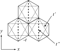
Figure 6: The $\pi$ flux model having additional hopping $t^{\prime\prime}$ (thick dashed lines) in the $y$ direction across the hexagon of the honeycomb lattice.

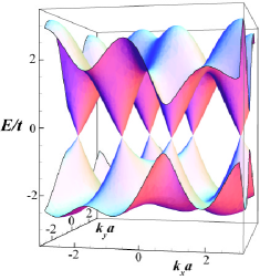
Figure 7: (Color online) Tilted Dirac cones for the $\pi$-flux model with $t"=t$ and $t^{\prime}/t=0.15$. The Dirac cones are located at $(k_{x},k_{y})=(\pi/2\sqrt{3}a,\pi/2a)$ and $(-\pi/2\sqrt{3}a,5\pi/6a)$ and $E=-0.3t$.

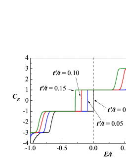
Figure 8: (Color online) The Chern number $C_{E}$ (Hall conductivity in units of $e^{2}/h)$ as a function of the Fermi energy $E/t$ in the presence of the next nearest-neighbor hopping $t^{\prime}$ for the $\pi$-flux model, for $\eta/a=1.5$, $\phi/\phi_{0}=1/36$, $\sigma/t=0.115$ and $(L_{x}/(\sqrt{3}a/2),L_{y}/(3a/2))=(18,12)$. The strength of the hopping $t"$ across the hexagon is assumed to be the average of $|t_{ij}|$ around the corresponding hexagon.

IV AC Hall effect

Now we would like to look at the ac extension of the Hall conductivity, i.e. optical Hall conductivity $\sigma_{xy}(\omega)$ to discuss the effect of the chiral symmetry. The crucial interests is whether the existence or otherwise of the chiral symmetry dominates ac responses as well, where we pay particular attention to the plateau structure in the optical Hall conductivity $\sigma_{xy}(\omega)$.

So we have calculated $\sigma_{xy}(\omega)$, where we solved the Hamiltonian containing various disorders with the exact diagonalization method, since we are interested in the localization effects in the ac Hall conductivity. We then compute the optical Hall conductivity by using the Kubo formula, since the method for calculating the topological (integer) Chern numbers in the dc case is not applicable to the optical conductivity. For the ac Hall conductivity, we consider the usual honeycomb lattice with different types of disorder to examine how the symmetry of disorder is reflected in the ac conductivity.

The Kubo formula for the ac conductivity is given as

$$\sigma_{xy}(\varepsilon_{F},\omega) = \frac{i\hbar}{L^{2}}\sum_{\epsilon_{a}<\varepsilon_{F}}\sum_{\epsilon_{b}\geq\varepsilon_{F}}\frac{1}{\epsilon_{b}-\epsilon_{a}}$$ (1)

$$\times \left(\frac{j_{x}^{ab}j_{y}^{ba}}{\epsilon_{b}-\epsilon_{a}-\hbar\omega}-\frac{j_{y}^{ab}j_{x}^{ba}}{\epsilon_{b}-\epsilon_{a}+\hbar\omega}\right),$$

where $\epsilon_{a}$ is the eigenenergy, $j_{x}^{ab}$ the current matrix elements between the eigenstates, and $\varepsilon_{F}$ the Fermi energy morimoto-opthall . The current operator is given by a gauge field derivative of the Hamiltonian as

$$\mbox{\boldmath$j$}=\frac{\partial H}{\partial\mbox{\boldmath$A$}},$$

where the gauge field and the Peierls phase in the Hamiltonians are related via $2\pi\theta_{ij}=\mbox{\boldmath$A$}\cdot(\mbox{\boldmath$r$}_{i}-\mbox{\boldmath$r$}_{j})$.

To see the effect of the chiral symmetry on $\sigma_{xy}(\omega)$, we have examined two cases: (i) The system with a site-potential disorder introduced as

$$H=\sum_{\langle i,j\rangle}-te^{-2\pi{\rm i}\theta_{ij}}c_{i}^{\dagger}c_{j}+{\rm h.c.}+\sum_{i}\delta\varepsilon_{i}c_{i}^{\dagger}c_{i},$$

with a random potential $\delta\varepsilon$ having a Gaussian distribution. The potential disorder, which breaks the chiral symmetry, models an effect of charged impurities in graphene samples. (ii) The system with random hopping,

$$H=\sum_{\langle i,j\rangle}(-t+\delta t_{ij})e^{-2\pi{\rm i}\theta_{ij}}c_{i}^{\dagger}c_{j}+{\rm h.c.},$$

which preserves the chiral symmetry, is considered to be coming from ripples in graphene samples. So we would look into the effect of these on the optical Hall conductivity.

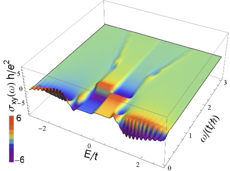
(a)

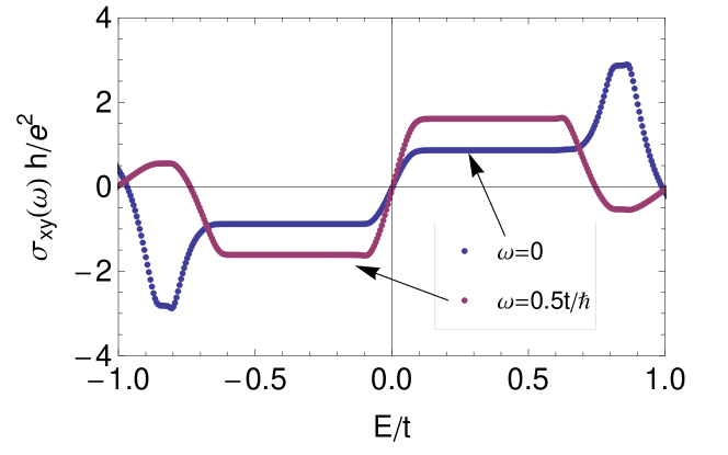
(b)

Figure 9: (a) $\sigma_{xy}(\varepsilon_{F},\omega)$ plotted against Fermi energy $\varepsilon_{F}$ and frequency $\omega$ for the honeycomb tight-binding model with a potential disorder $\sqrt{\langle\delta\varepsilon^{2}\rangle}=0.1t$ which breaks the chiral symmetry. (b) $\sigma_{xy}(\varepsilon_{F},\omega)$ for $\omega=0,0.5t/\hbar$ is displayed to show the broadening of the step structure associated with the $n=0$ Landau level. The parameters are $\phi/\phi_{0}=1/18$, $(L_{x}/(\sqrt{3}a/2),L_{y}/(3a/2))=(27,24)$.

Fig.9 shows $\sigma_{xy}(\varepsilon_{F},\omega)$ plotted against Fermi energy $\varepsilon_{F}$ and frequency $\omega$ with a potential disorder $\sqrt{\langle\delta\varepsilon^{2}\rangle}=0.1t$ which breaks the chiral symmetry. The curve for $\omega=0$ in Fig.9(a) corresponds to dc Hall conductivity. If we vary Fermi energy $\varepsilon_{F}$ for a fixed frequency $\omega$, we notice that there are two distinct regions. For the Dirac-cone-like energy region bounded by the van Hove singularities ($|\varepsilon_{F}|<t$) we observe step structures at Dirac Landau levels, where we have wider plateaus for higher Landau levels due to a $\sqrt{B}$ dependence of cyclotron energy for Dirac QHE. At the van Hove singularities the Dirac QHE crosses over to the ordinary QHE for usual fermions around the band edges, and outside the van Hove singularities ($|\varepsilon_{F}|>t$) an usual QHE step sequence is recognized.

If we look at the dependence on the frequency $\omega$, each plateau exhibits the cyclotron resonance behavior as $\omega$ is increased, where the resonance shape differs between the two regions. For the usual QHE region the resonance occurs for small $\omega$ because of small cyclotron frequency ($\propto B$). In the Dirac QHE region, we have resonances for larger $\omega$ $(\propto\sqrt{B})$, which appear at various resonance frequencies that correspond to resonances between different for LL’s with non-uniform LL spacings with a peculiar selection rule, $|n|\leftrightarrow|n+1|$ for Dirac QHE. An interesting point observed for the honeycomb tight-binding model is that these two regions emerge from the nature of the honeycomb band dispersion and separated by van Hove singularities.

Fig.9(b) depicts the step structure around $n=0$ LL for dc and ac ($\omega=0.5t/\hbar$) Hall conductivities, which shows that the $n=0$ steps are blurred both for dc and ac response when the disorder does not respect the chiral symmetry.

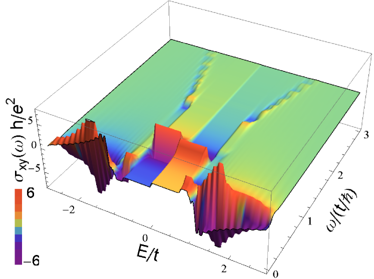
(a)

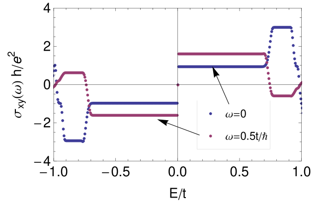
(b)

Figure 10: (a) $\sigma_{xy}(\varepsilon_{F},\omega)$ plotted against Fermi energy $\varepsilon_{F}$ and frequency $\omega$ for the honeycomb tight-binding model with random hopping $\sqrt{\langle\delta t^{2}\rangle}=0.1t$ which respects the chiral symmetry. (b) $\sigma_{xy}(\varepsilon_{F},\omega)$ with $\omega=0,0.5t/\hbar$ is displayed to show the anomalous step structure at n=0 LL retained for ac Hall conductivity. The parameters involved are $\eta/a=2.0$, $\phi/\phi_{0}=1/18$, $(L_{x}/(\sqrt{3}a/2),L_{y}/(3a/2))=(27,24)$.

Now we come to the original question of what happens to the ac Hall conductivity when the disorder respects the chiral symmetry. Figure 10 shows $\sigma_{xy}(\varepsilon_{F},\omega)$ for the case of a random hopping $\sqrt{\langle\delta t^{2}\rangle}=0.1t$ which respects the chiral symmetry. The overall structure of the $\sigma_{xy}(\varepsilon_{F},\omega)$ is similar to the random potential case, but we can immediately notice that the $n=0$ step in $\sigma_{xy}(\varepsilon_{F},\omega)$ exhibits an anomalously sharp step structure at even for the optical Hall conductivity as in the dc Hall conductivity. Indeed, Fig.10(a) indicates that $\sigma_{xy}(\varepsilon_{F}=0,\omega)$ shows a sharp step for all the values of $\omega$, which should come from the protected $n=0$ LL by the chiral symmetry.

We can conclude that the chiral symmetry and the zero mode protection give a crucial effect on the ac response of the system as in the dc response, where the presence of the chiral symmetry gives a rise to the anomalously sharp step structure in $\sigma_{xy}(\varepsilon_{F},\omega)$ associated with delta-function like $n=0$ LL. The honeycomb lattice calculation, performed here for the optical Hall conductivity, is not only more realistic than the effective Dirac field description, but also reveals an existence of two regions (Dirac QHE and usual fermionic QHE) coming from the van Hove singularity in the band dispersion, where totally different plateau width and cyclotron resonance structures are observed.

V Conclusions

We have investigated, based on several lattice models, the relationship between the chiral symmetry and the anomalous criticality associated with the $\delta$-function like density of states at the $n=0$ Landau level in graphene, which yields a step-function like Hall plateau transition. The ac as well as dc Hall conductivity has been examined as a function of the Fermi energy in the presence of the spatially-correlated chiral symmetric bond disorder. For the dc Hall conductivity, it has been shown that the anomalous criticality is surprisingly robust against the introduction of the next-nearest neighbor hopping in the honeycomb lattice, which is considered to be appreciable in real graphene. The anomalous criticality may therefore be realized in a suspended clean graphene where ripples are the major disorder. As for the symmetry, the present results implies that the anomalous criticality can be insensitive to the breakdown of the usual chiral symmetry as long as the effective chiral symmetry that produces the massless Dirac cones is preserved. We have also shown that the anomaly is robust against a slight tilt in the Dirac cones, which suggests the possibility to observe the anomalous criticality not only in graphene but also in organic materials. For the ac Hall conductivity, we have shown that even for finite frequencies, the transition at the $n=0$ Landau level exhibits the anomalous criticality, with the robust plateau structure retained for long-ranged, chiral-symmetric bond disorders. Based on these numerical results, we conclude that the chiral symmetry manifests itself both in the dc and the ac Hall transitions yielding the anomalous criticality at the $n=0$ Landau level of graphene.

- (1) K.S. Novoselov et al, Nature 438, 197 (2005).
- (2) Y. Zhang, Y.W. Tan, H.L. Stormer and P. Kim, Nature 438, 201 (2005).
- (3) Y. Zheng and T. Ando, Phys. Rev. B 65, 245420 (2002).
- (4) M. Koshino and T. Ando, Phys. Rev. B 75, 033412 (2007).
- (5) L. Schweitzer and P. Markoš, Phys. Rev. B 78, 205419 (2008).
- (6) P.M. Ostrovsky, I.V. Gornyi, and A.D. Mirlin, Phys. Rev. B 77, 195430 (2008).
- (7) T. Kawarabayashi, Y. Hatsugai, and H. Aoki, Phys. Rev. Lett. 103, 156804 (2009); Physica E42, 759 (2010).
- (8) Y. Hatsugai, T. Fukui, and H. Aoki, Phys. Rev. B 74, 205414 (2006); Eur. Phys. J. Special topics, 148, 133 (2007).
- (9) Y. Hatsugai, Solid State Comm. 149 (2009) 1061; S. Ryu and Y. Hatsugai, Phys. Rev. Lett. 89, 077002 (2002).
- (10) J.C. Meyer et al, Nature 446, 60 (2007).
- (11) V. Geringer, M. Liebmann, T. Echtermeyer, S. Runte, M. Schmidt, R. Rückamp, M.C. Lemme, and M. Morgenstern, Phys. Rev. Lett. 102, 076102 (2009).
- (12) K. Nomura et al, Phys. Rev. Lett. 100, 246806 (2008).
- (13) A.H. Castro Neto et al, Rev. Mod. Phys. 81, 109 (2009).
- (14) S. Reich, J. Maultzsch, C. Thomsen, and P. Ordejón, Phys. Rev. B 66, 035412 (2002).
- (15) T. Nakajima and H. Aoki, Physica E 40, 1354 (2008).
- (16) J.C. Slonczewski and P.R. Weiss, Phys. Rev. 109, 272 (1958).
- (17) S. Katayama, A. Kobayashi, and Y. Suzuura, J. Phys. Soc. Jpn. 75, 054705 (2006).
- (18) N. Tajima, S. Sugawara, M. Tamura, Y. Nishio, and K. Kajita, J. Phys. Soc. Jpn. 75, 051010 (2006).
- (19) D.J. Thouless et al, Phys. Rev. Lett. 49, 405 (1982).
- (20) Q. Niu, D.J. Thouless, and Y.S. Wu, Phys. Rev. B 31, 3372 (1985).
- (21) Y. Hatsugai, Phys. Rev. Lett. 71, 3697 (1993).
- (22) H. Aoki and T. Ando, Phys. Rev. Lett. 57, 3093 (1986).
- (23) Y. Hatsugai, J. Phys. Soc. Jpn. 73, 2604 (2004); ibid 74, 1374 (2005).
- (24) T. Fukui, Y. Hatsugai, and H. Suzuki, J. Phys. Soc. Jpn. 74, 1674 (2005).
- (25) Y. Hatsugai, T. Fukui, and H. Suzuki, Physica E 34, 336 (2006).
- (26) R.D. King-Smith and D. Vanderbilt, Phys. Rev. B 47, 1651 (1993).
- (27) H. Song, I. Maruyama, and Y. Hatsugai, Phys. Rev. B76, 132202 (2007).
- (28) T. Morimoto, Y. Hatsugai, and H. Aoki, Phys. Rev. B 78, 073406 (2008).
- (29) M. L. Sadowski, G. Martinez, M. Potemski, C. Berger, and W. A. de Heer, Phys. Rev. Lett. 97, 266405 (2006).
- (30) T. Morimoto, Y. Hatsugai and H. Aoki, Phys. Rev. Lett. 103, 116803 (2009).
- (31) Y. Ikebe, T. Morimoto, R. Masutomi, T. Okamoto, H. Aoki, and R. Shimano, Phys. Rev. Lett. 104, 256802 (2010).
- (32) A. Altland and M.R. Zirnbauer, Phys. Rev. B 55, 1142 (1997).
- (33) T. Kawarabayashi et al, Phys. Rev. B 75, 235317 (2007); Phys. Rev. B 78, 205303 (2008).
- (34) Y. Hatsugai, K. Ishibashi, and Y. Morita, Phys. Rev. Lett. 83, 2246 (1999).
- (35) Y. Morita and Y. Hatsugai, Phys. Rev. Lett. 79, 3728 (1997); Y. Hatsugai, X.-G. Wen, and M. Kohmoto, Phys. Rev. B 56, 1061 (1997).