Universal occurrence of mixed-synchronization in counter-rotating nonlinear coupled oscillators

Abstract

By coupling counter–rotating coupled nonlinear oscillators, we observe a “mixed” synchronization between the different dynamical variables of the same system. The phenomenon of amplitude death is also observed. Results for coupled systems with co–rotating coupled oscillators are also presented for a detailed comparison. Results for Landau-Stuart and Rössler oscillators are presented.

Natural systems are rarely isolated, and thus studies of coupled dynamical systems which arise in a variety of contexts in the physical, biological, and social sciences, have broad relevance to many areas of research.

Consider the coupling of two nonlinear oscillators, schematically shown in Fig. 1, with the symbols ‘+’ and ‘–’ indicating the sense of rotation of the orbits in the phase space, namely clockwise or counter-clockwise. If directions of rotation of both oscillators are the same, as in Fig. 1(a), the system is co-rotating: such coupled nonlinear oscillators have been extensively studied from both theoretical and experimental points of view synch .

Important phenomena which have been observed for co-rotating oscillators include synchronization, hysteresis, phase locking, phase shifting, phase-flip, or riddling synch ; kaneko ; ott ; cs ; hys ; ap . There are many forms of synchrony e. g. complete synchronization: system variables become identical cs , phase synchronization: phase difference between the oscillators becomes bounded ps , and others e. g. lag synchronization and generalized synchronization etc. synch . In all these type of synchronizations if one of the dynamical variable is synchronized then rest of the variables follow the same.

Another important property of co-rotating oscillators is amplitude death (AD) bar where amplitude of the oscillation ceases to zero at stable fixed point of the system. This AD can be achieved with various type of interactions between the oscillators e. g. mismatched oscillators ins , delayed reddy , conjugate rajat and nonlinear mukesh etc.

When the rotations of the individual oscillators are in opposite senses, as in Fig. 1(b), then the system is termed counter-rotating. To the best of our knowledge, counter-rotating systems have not explicitly been studied earlier, and in this Letter, we focus on such systems. We observe that both AD as well as synchronization arise with this form of coupling. A novel “mixed” type of synchronization among different variables is seen to occur: some variables are synchronized in-phase while other variables can be out-of-phase.

Figure 1: Schematic coupling schemes for two coupled oscillators: (a) co-rotating and (b) counter-rotating. Arrows show the directions of rotation while $-$ and $+$ indicate the corresponding clockwise and anticlockwise rotations respectively. H denotes the coupling function, Eq. (1).

Consider a coupled system of $N$ nonlinear oscillators specified by the equations

$$\dot{\mathbf{X}}_{i}=\mathbf{F}_{i}(\mathbf{X}_{i},\omega_{i})+\frac{\epsilon}{K_{i}}\sum_{j=1}^{K_{i}}A_{ij}\mathbf{H}(\mathbf{X}_{i},\mathbf{X}_{j}),~{}~{}i=1,\ldots,N$$ (1)

where $\mathbf{X}_{i}$ is $m$-dimensional vector of dynamical variables and the $\mathbf{F}_{i}$’s specify the evolution equations of the different oscillators with internal frequency parameter $\omega_{i}$. Here $K_{i}$ is the number of connections to the $i-$th oscillators, namely its degree such that $1\leq K_{i}<N$, and $\epsilon$ is the coupling strength. The connection topology is specified by the adjacency matrix ${\bf A}$, with $A_{ij}=1$ if oscillators $i$ and $j$ are connected to each other and $A_{ij}=0$ otherwise. The coupling function $\mathbf{H}:{\mathbb{R}}^{m}\to{\mathbb{R}}^{m}$ specifies the manner in which the oscillators $i$ and $j$ are coupled, with $\mathbf{H}(\mathbf{X}_{i},\mathbf{X}_{j})$ being a function of $\mathbf{X}_{i}$ and $\mathbf{X}_{j}$.

We first analyze two Landau–Stuart limit cycle oscillators ap coupled in the co– (Fig. 1(a)) as well as counter-rotating (Fig. 1(b)) schemes. The coupled equations are

$$\dot{Z}_{i} = (1+i\omega_{i}-|Z_{i}|^{2})Z_{i}+\epsilon(Z_{j}-Z_{i})$$ (2)

where $i,j=1,2$, $i\neq j$ and $Z_{i}$ is the complex variables with real part $x_{i}$ and imaginary part $y_{i}$. In Eq. (1) the variables are $X_{i}=[x_{i},y_{i}]^{T}$ and $H=[(x_{j}-x_{i}),(y_{j}-y_{i})]^{T}$ where $T$ denotes the transpose. In the uncoupled case, i.e. $\epsilon=0$, each oscillator has a fixed point at $Z_{*j}=0$ which is unstable with eigenvalues $1\pm i\omega_{j}$. Irrespective of the values of $\omega_{j}$ each oscillator has the same attractor with unit radius, and corresponding frequency $\omega_{j}$. Shown in Fig. 2 (a) and (b) are the transient trajectories for co– ($\omega_{1}=\omega_{2}=5$) and counter-rotating ($\omega_{1}=5,\omega_{2}=-5$) respectively for two uncoupled oscillators. These clearly show that, in these two cases, the trajectories are moving in the same or in the opposite directions respectively. In order to see the effects of coupling on these both schemes, results for co– and counter rotating coupled oscillators are shown in the left and the right panels respectively in Fig. 2. As the coupling is introduced, the dynamical behavior changes. The few largest Lyapunov exponents (see Fig. 2(c,d)) clearly show that in the case of co-rotating oscillators, the largest Lyapunov exponent remains zero for all coupling strengths which suggests the continuation of periodic motion. This is shown Fig. 2(e) at $\epsilon=0.5$. However for counter-rotating oscillators, the maximal Lyapunov exponent (Fig. 2(d)) becomes negative (this is an instance of amplitude death, marked “AD”) where the fixed point $Z_{*1}=Z_{*2}=0$ is stabilized. A simple eigenvalue ($\lambda$) calculation, with real part $\alpha$ and imaginary part $\beta$, gives the relation,

$$\alpha=1-\epsilon\pm\epsilon\mbox{~{}~{}and~{}~{}}\beta=\omega$$ (3)

where $\omega_{1}=\omega_{2}=\omega$ for co-rotation (left panel). For co-rotating coupled oscillators the real part of the largest eigenvalue, $\alpha=1$, and hence fixed point will be unstable for all values of $\omega$ and $\epsilon$. This rules out the possibility of AD in such scheme (for details see Ref. ins ). However for $\omega_{1}=\omega,\omega_{2}=-\omega$ for the case of counter–rotating oscillators (right panel) the eigenvalues will be

$$\alpha=1-\epsilon\mbox{~{}~{}and~{}~{}}\beta=\sqrt{\omega^{2}-\epsilon^{2}}$$ (4)

for $\epsilon<\omega^{2}$, while

$$\alpha=1-\epsilon\pm\sqrt{\epsilon^{2}-\omega^{2}}\mbox{~{}~{}and~{}~{}}\beta=0,$$ (5)

for $\epsilon^{2}>\omega^{2}$. These relations give the region $1<\epsilon<(1+\omega^{2})/2$ where the fixed point at the origin will be stable ($\alpha<0$) as shown in Fig. 2(d) by the arrow. The transient trajectory in AD region at $\epsilon=2$ is shown in the inset figure. This clearly shows, which is a new result, that AD is possible (via a Hopf bifurcation) in the counter-rotating identical oscillators while it is impossible in the co-rotating case. It should be noted that AD is possible in co-rotating case only when there are mismatch in frequencies of the oscillators ins . Here we show that in counter-rotating case everything is same as that of the co-rotating except directions of rotation. This novel result clearly distinguishes counter-rotating oscillators from the more extensively studied co-rotating case.

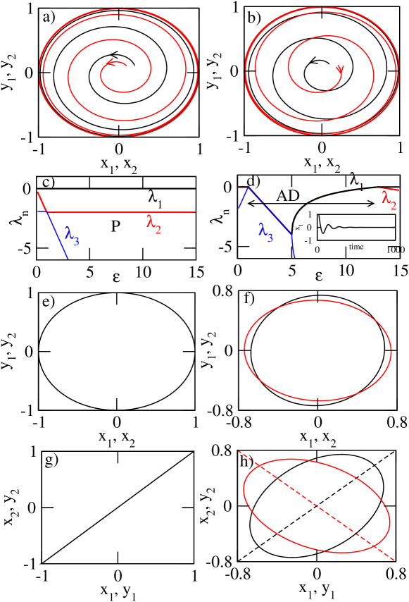
Figure 2: Left and right panels correspond to the co- and counter-rotating respectively Landau-Stuart oscillators, Eq. (2). (a,b) The transient trajectories of uncoupled oscillators. (c,d) A few largest Lyapunov exponents with coupling strength, $\epsilon$. Inset figure in (d) corresponds to the transient trajectories in AD regime at $\epsilon=2$. (e,f) The asymptotic attractors in $x_{i}-y_{i}$ plane. (g,h) The signature of relative phase in $x_{1}$ vs $x_{2}$ and $y_{1}$ vs $y_{2}$ at $\epsilon=0.5$. Dashed lines in (h) show the relative phase-difference of $0$ (black) and $\pi$ (red).

Another important result pertains to the regime of synchronized motion. Figure 2(e) shows the attractors which are exactly same as uncoupled case (Fig. 2(a)) having complete synchronization. The relative phase between the oscillators is shown in Fig. 2(g) where trajectories lie on the synchronization manifold, $x_{1}=x_{2},y_{1}=y_{2}$; this confirms the occurrence of complete synchronization. However in the counter-rotating case, Fig. 2(f) the attractors are not identical: they do not remain as limit cycle circles (with unit radius) instead change shape as well as get reduced in amplitude. The oscillators are synchronized though, as can be seen in the relative phase shown in Fig. 2(h). The $x-$ variables essentially in-phase while $y-$ variables are out-of-phase (dashed lines correspond to the relative phase zero (black) and $\pi$ (red)). The simultaneous presence of nearly in- as well as out-of-phase synchrony in different variables among the same oscillators is termed here as “mixed” synchronization.

It is important to note that the usual definition of phase difference between oscillators is not applicable here since there is continuous change of individual angle in opposite directions. Therefore the effect of counter-rotation has drastic difference due to presence of mixed-synchronization as compared to co-rotation.

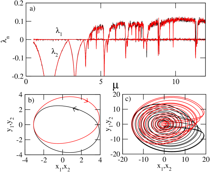
Figure 3: (a) The largest two Lyapunov exponents with internal parameter, $\mu,$ for anticlockwise ($\omega_{1}=1$ – black lines) and clockwise ($\omega_{2}=-1$ – red lines) for uncoupled ($\epsilon=0$) Rössler oscillators, Eq. (6). The trajectories of individual oscillators for (b) periodic ($\mu=2$) and (c) chaotic ($\mu=10$) motions.

The generality of these results is demonstrated in a system of coupled Rössler oscillators ross , given by the equations of motion

$$dx_{i}(t)\over dt = -\omega_{i}y_{i}-z_{i}+\epsilon(x_{j}-x_{i})$$

$$dy_{i}(t)\over dt = \omega_{i}x_{i}+0.2y_{i}$$

$$dz_{i}(t)\over dt = 0.2+z_{i}(x_{i}-\mu)$$ (6)

where $\omega_{i}$ (internal frequency) and $\mu$ are parameters, and $i,j=1,2$, $i\neq j$. (With regard to Eq. (1), $X_{i}=[x_{i},y_{i},z_{i}]^{T}$ and $H=[(x_{j}-x_{i}),0,0]^{T}$.)

Changing the parameter $\omega_{i}$ merely changes the sense of rotation; as can be seen in Fig. 3(a) the two largest Lyapunov exponents as a function of $\mu$ are essentially identical for $\omega_{1}=1$ (black curves) and $\omega_{2}=-1$ (red curves). Corresponding typical trajectories for periodic and chaotic motions are shown in Fig. 3(b) and (c) at $\mu=2$ and $10$ respectively. Note that there is change of position of the attractors in the phase space. These fixed points $(x_{*i}=(\mu\pm\sqrt{\mu^{2}-0.16/{\omega_{i}^{2}}})/2,y_{*i}=5\omega_{i}x_{*i},z_{*i}=5\omega_{i}^{2}x_{*i})$ depend on the sign of $\omega_{i}$ (unlike the case of Eq. (2) where the origin fixed point is independent of frequency).

The change in dynamical behavior arising from the coupling is shown in Fig. 4 for co– (left panel) and counter–rotating (right panel) coupled chaotic ($\mu=10$) Rössler oscillators, Eq. (6). For small coupling, say $\epsilon=0.005$, the motion is unsynchronized which can be seen from the relative phase between the trajectories in Fig. 4(c) in $x_{1}$ vs $x_{2}$ (black) and $y_{1}$ vs $y_{2}$ (red). As the coupling strength is increased beyond $\epsilon\sim 0.02$ phase-synchronization sets in (the fourth largest Lyapunov exponent (in green) becomes negative ps ), and after this all variables $x,y,z$ remain in–phase as shown in Fig. 4(e). When the coupling is increased beyond $\epsilon\sim 0.12$ complete synchronization occurs ps as seen in Fig. 4 (g) where $x_{1}=x_{2},y_{1}=y_{2}$.

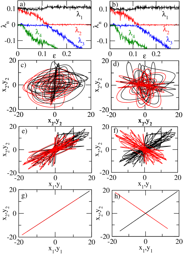
Figure 4: Left and right panels correspond to the co- and counter-rotating chaotic Rössler oscillators respectively, Eq. (6). (a,b) A few largest Lyapunov exponents with coupling strength, $\epsilon$ at $\mu=10$. The signature of (c,d) non-synchronization, (e) phase-synchronization, (f) mixed-synchronization, (g) complete-synchronization and (h) mixed-synchronization. The coupling strengths for (c,d), (e,f) and (g,h) are at $\epsilon=0.005,0.05$ and $0.2$ respectively.

For counter-rotating oscillators ($\omega_{1}=1,\omega_{2}=-1$) (right panel) Lyapunov spectrum (Fig. 4(b)) remains the same as for co-rotating oscillators (Fig. 4(a)) showing that the invariant measure does not change. For small coupling the oscillators are not in the phase synchronized state Fig. 4(d), as analogous to the co-rotating case Fig. 4(c). However, as coupling is increased further, the phase synchronization sets in, (Fig. 4(f)), but the relative phase between the three variables is not identical.

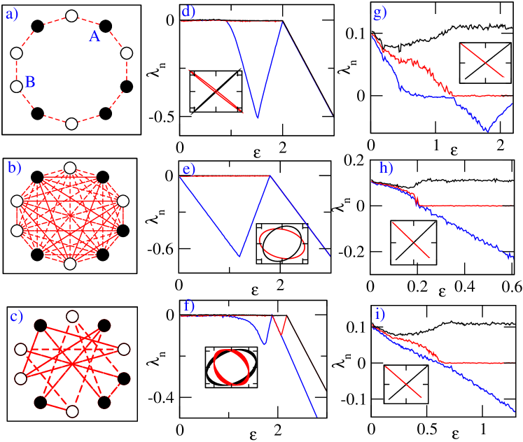
Figure 5: Left panel shows the network of different topologies for $N=10$ coupled oscillators: (a) periodic chain (b) globally coupled and (c) small-world network–see the text for details. The largest three Lyapunov exponents with coupling strength for different topologies are plotted in the middle and right panel corresponding to the Landau-Stuart and the Rössler coupled oscillators respectively. Inset figures show the relative phase of $x_{A}$ vs $x_{B}$ (black) and $y_{A}$ vs $y_{B}$ (red) between the marked oscillators A and B. The coupling strengths for the inset figures of middle panels (d,e,f) are at $\epsilon=1.5$ while the corresponding values for (g), (h) and (i) are at $\epsilon=2,0.5$ and $1$ respectively.

Shown in Fig. 4 (f) is the relative phase in $x_{1}-x_{2}$ and $y_{1}-y_{2}$ planes. Clearly $x_{1}$ and $x_{2}$ are in–phase (black) synchronized while $y_{1}$ and $y_{2}$ are out-of-phase (red). This is clearer for higher coupling, $\epsilon=0.2$ (Fig. 4(h)) where there is complete synchronization in $x_{1}$ and $x_{2}$ (zero relative phase) while $y_{1}$ and $y_{2}$ remain out-of-phase with phase difference $\pi$. We find $z_{1}$ and $z_{2}$ in complete synchrony (results not shown here new ). For counter-rotating coupled oscillators it appears that if one variable is in-phase synchrony, then at least one other variable must be out-of-phase, i.e. if motion is on the manifold ($x_{1}=x_{2},y_{1}=y_{2},z_{1}=z_{2}$) for co-rotating case (Fig. 4(g)) then the corresponding manifold for the counter-rotating case is ($x_{1}=x_{2},y_{1}=-y_{2},z_{1}=z_{2}$), Fig. 4(h).

Mixed-synchronization and AD also occur in network of oscillators where the rotation sense is chosen randomly. We present representative results for $N=10$ for Landau-Stuart and Rössler oscillators in middle and right panels respectively in Fig. 5. The rotations of individual oscillators are indicated in Fig. 5(a,b,c) where open and filled circles correspond to the clockwise and anticlockwise rotations respectively in these particular realizations. Three different topologies are taken: (i) nearest neighbor coupling with periodic boundary conditions ($K=2$)–Fig. 5(a); (ii) global coupling where each oscillator is coupled with all others $(K=N-1)$ – see Fig. 5(b); (iii) each oscillator is coupled to three ($K=3$) random nodes — see Fig. 5(c) which realizes a small world topology sw . The coupling functions $H$ for these network of oscillators are the same as in Figs. 2 and 4 for Landau-Stuart and Rössler oscillators respectively. In Figs. 5(d) to (i) the largest few Lyapunov exponents are plotted as a function of the coupling strength in the three cases. The inset figures in Fig. 5(d-i) show the relative phase $x_{A}$ vs $x_{B}$ (black curves) and $y_{A}$ vs $y_{B}$ (red curves) for counter-rotating oscillators between the marked oscillators A and B in (a) verifying the existence of mixed-synchronization for both systems. The occurrence of AD is also observed in networks of Landau-Stuart oscillators, as shown by negative Lyapunov exponents in the middle panel.

In summary, we have observed the universal occurrence of mixed-synchronization in counter-rotating oscillators: some variables are synchronized in-phase, while others are out-of-phase. The phenomenon of amplitude death is also observed in some cases, as for example, the Landau-Stuart limit cycle oscillators studied here. These results are also found to persist in networks of oscillators of different topologies. We have also checked that these results persist under parameter mismatch new , and believe that they are generally applicable and should be observable in experiments. Thus the phenomena observed here will occur in other coupled systems as well.

In this paper we have considered only linear diffusive coupling, and other types of interactions such as one-way, conjugate rajat , and nonlinear couplings mukesh are still need to be explored. Dynamical phenomena such as riddling, hysteresis, phase locking, phase-shifting, phase-flip synch ; kaneko ; ott ; cs ; hys ; ap etc. which have been seen in co-rotating coupled systems should also be explored in counter-rotating coupled oscillators.

This work is supported by the Delhi University and the Department of Science and Technology, Government of India. I thank R. Ramaswamy for his comments on this paper.

References

- (1) A. Pikovsky, M. Rosenblum, and J. Kurths, Synchronization, A universal concept in nonlinear science, Cambridge University Press, Cambridge, 2001.
- (2) K. Kaneko, Theory and Applications of Coupled Map Lattices, Wiley, New York, 1993.
- (3) E. Ott, Chaos in Dynamical Systems, Cambridge University Press, Cambridge, 1993.
- (4) L. Pecora and T. Carroll, Synchronization in chaotic systems, Phys. Rev. Lett. 64 (1990) 821-824.
- (5) A. Prasad,L. D. Iasemidis, S. Sabesan and K. Tsakalis, Dynamical hysteresis and spatial synchronization in coupled nonidentical chaotic oscillators, Pramana J. Phys., 64 (2005) 513-523.
- (6) A. Prasad, Amplitude Death in coupled chaotic oscillators, Phys. Rev. E, 72 (2005) 056204-10; A. Prasad, J. Kurths, S. K. Dana, and R. Ramaswamy, Phase-flip bifurcation induced by time delay, Phys. Rev. E, 74 (2006) 035204-4; Universal occurrence of the phase-flip bifurcation in time-delay coupled systems, CHAOS, 18 (2008) 023111-8.
- (7) M. G. Rosenblum, A. S. Pikovsky, and J. Kurths, Phase synchronization of chaotic oscillators, Phys. Rev. Lett. 76 (1996) 1804-1807.
- (8) K. Bar-Eli, On the stability of coupled chemical oscillators, Physica D, 14 (1985) 242-252.
- (9) D. G. Aronson, G. B. Ermentrout and N. Kopell, Amplitude response of coupled oscillators, Physica D, 41 (1990) 403-449.
- (10) D. V. Ramana Reddy, A. Sen, and G. L. Johnston, Time delay induced death in coupled Limit Cycle oscillators, Phys. Rev. Lett., 80 (1998) 5109-5112.
- (11) R. Karnatak, R. Ramaswamy and A. Prasad, Amplitude death in the absence of time delays in identical coupled oscillators, Phys. Rev. E, 76 (2007) 035201-4; Synchronization regimes in conjugate coupled chaotic oscillators, CHAOS, 19 (2009) 033143-5.
- (12) A. Prasad, M. Dhamala, B. M. Adhikari and R. Ramaswamy, Amplitude death in nonlinear oscillators with nonlinear coupling, Phys. Rev. E, 81 (2010) 027201-4; Targeted control of amplitude dynamics in coupled nonlinear oscillators, Phys. Rev. E (2010)-in press.
- (13) O. E. Rössler, An equation for continuous chaos, Phys. Lett. A, 57 (1979) 397-398.
- (14) A. Prasad, in preparation.
- (15) D. J. Watts and S. H. Strogatz, Collective dynamics of small-world networks, Nature, 393 (1998) 440-442.