Deformation-induced accelerated dynamics in polymer glasses

Abstract

Molecular dynamics simulations are used to investigate the effects of deformation on the segmental dynamics in an aging polymer glass. Individual particle trajectories are decomposed into a series of discontinuous hops, from which we obtain the full distribution of relaxation times and displacements under three deformation protocols: step stress (creep), step strain, and constant strain rate deformation. As in experiments, the dynamics can be accelerated by several orders of magnitude during deformation, and the history dependence is entirely erased during yield (mechanical rejuvenation). Aging can be explained as a result of the long tails in the relaxation time distribution of the glass, and similarly, mechanical rejuvenation is understood through the observed narrowing of this distribution during yield. Although the relaxation time distributions under deformation are highly protocol specific, in each case they may be described by a universal acceleration factor that depends only on the strain.

I Introduction

Although it has long been recognized that mechanical deformation can modify the structural relaxation dynamics of polymer glasses, obtaining a complete picture of the deformation-induced mobility remains an important challenge. It is most often assumed that mechanical stress lowers the activation barriers to molecular mobility, thereby allowing the solid to yield and flow. This simple idea, first proposed by Eyring in 1936 Eyring (1936), remains the central tenet of several models of plasticity in amorphous solids Tervoort et al. (1996); Chen and Schweizer (2007). Other control variables have also been proposed to explain the increased molecular mobility under deformation. In the Soft Glassy Rheology (SGR) model, activated barrier crossings are accelerated by the local strain on mesoscopic regions of the glass Sollich et al. (1997); Fielding et al. (2000). In the Shear Transformation Zone (STZ) theory, deformation is caused by a population of bistable states (shear transformation zones) that can flip from one orientation to another in response to stress Falk and Langer (1998); Langer (2006). The stress induced transition between the bistable states is modeled using a variant of the Eyring model, and the population of shear transformation zones is controlled by an effective temperature which explicitly depends on the strain rate $\dot{\epsilon}$ Langer (2004); Langer and Manning (2007). Still other models have proposed the free volume Struik (1978), and the configurational entropy Lustig et al. (1996) as the important variables to describe the deformation-induced mobility. There is clearly no consensus on the correct way to think about deformation in glasses.

Experimentally, the structural relaxation times of deformed polymer glasses have traditionally been studied through rheological measurements, where the segmental dynamics are inferred from the mechanical response Struik (1978); Martinez-Vega et al. (2002); O’Connell and McKenna (2002); McKenna and Zapas (1986); Waldron et al. (1995). In recent years, experiments and simulations have allowed researchers to directly probe the microscopic segmental dynamics during deformation. Solid-state NMR experiments examined the dynamics of glassy Nylon-6 near $T_{g}$ under uniaxial extension and found significant deformation-induced mobility near yield Loo et al. (2000). Lee et al. performed a series of experiments investigating the segmental relaxation dynamics in solid poly(methyl methacrylate) through an optical photobleaching technique that probes the reorientation of small dye molecules embedded in the polymer matrix during a step stress (creep) experiment Lee et al. (2008, 2009). Relaxation times were found to be significantly accelerated compared to the undeformed sample, and in fact the segmental mobility was close to linearly correlated with the strain rate. During plastic flow, the distribution of relaxation times was also narrowed, which was interpreted as evidence that the dynamics has become more homogeneous.

Molecular dynamics simulations have confirmed these results through direct measurement of the segmental dynamics. Lyulin et al. performed simulations on united atom models for polystyrene and polycarbonate during constant strain rate deformation Lyulin et al. (2005). The segmental mobility was monitored through the monomer mean-squared displacement and increased dramatically beyond the yield point. Similarly, simulations of polyethylene under compressive strain showed that the dihedral transition rate in between trans/gauche states was increased due to the deformation even in the sub-yield regime Capaldi et al. (2002). Several simulation studies have also confirmed the strong correlation between the relaxation time and strain rate that has been seen in experiment. Riggleman et al. simulated a bead-spring polymer glass during non-linear creep Riggleman et al. (2007, 2008). The covalent bond autocorrelation and intermediate scattering functions both decayed more rapidly in the deformed sample, and it was found that the segmental mobility was strongly correlated to the strain rate under both tensile and compressive loading.

For polymer glasses in particular, the effects of physical aging further complicate the analysis of the dynamics under deformation, as the mechanical response depends sensitively on the history of the glass. Non-equilibrium relaxations cause relaxation times to grow, and hence the glass becomes stiffer with the time since it was formed. Since the age of a sample is often characterized by its relaxation times, the deformation-induced acceleration of the dynamics has been associated with “mechanical rejuvenation” of aging glasses Struik (1978). Indeed, in the post-yield flow regime, all history dependence is erased. Hasan and Boyce investigated this phenomenon using differential scanning calorimetry on polymer glasses during constant strain rate deformation Hasan and Boyce (1993). While, at sub-yield strains, the aged glasses exhibited different mechanical properties and enthalpies, these differences were found to disappear once the glasses began to flow. Simulations have provided further insight into the nature of rejuvenation. Utz et al. found that the history dependence of the inherent structure energies and the pair correlation functions of the binary metallic Lennard-Jones glass (BMLJ) were also erased during yielding Utz et al. (2000). Post-yield, these parameters took values more typical of rapidly quenched, or unaged samples. Further analysis, however, seems to indicate that the rejuvenated glass is not truly the same as a younger glass Lacks and Osborne (2004); Lyulin and Michels (2007).

Below yield, the claim of mechanical rejuvenation is even more controversial McKenna (2003). In this regime, deformation increases molecular mobility at the same time as aging decreases it Lee (2009), and experiments show that both the volume Lee and McKenna (1990) and the relaxation times Lee (2009) of the glass quickly return to their previous states once the load is removed Warren and Rottler (2008). In this report, we reserve the term “rejuvenation” for the erasure of aging due to deformation, without comment on whether the yielded state truly resembles a younger glass or is something else altogether.

Mobility and aging in previous studies has been measured using spatially averaged correlation and response functions; however, it is becoming increasingly clear that glasses are both dynamically and mechanically heterogeneous. A number of simulations have studied the spatial heterogeneity of structural relaxations under deformation in the limit of low temperatures and small shear rates C. and Lemaitre (2004); Tanguy et al. (2006). Results show that the elementary relaxations responsible for plastic deformation are strongly localized, involving a region of several diameters across. They are also intermittent: rapid relaxation events are separated by periods of perfectly affine deformation. Furthermore, the stress and elastic modulus are also locally heterogeneous Tsamados et al. (2009); Yoshimoto et al. (2004) and structural relaxations occur predominantly in weak regions of the glass Tsamados et al. (2009).

We use molecular dynamics simulations of an aging polymer glass to investigate the complex interaction between aging and deformation at the microscopic level, and to identify the deformation variables important to the description of the deformation-induced mobility. Three deformation protocols are employed: a step stress (creep), a constant strain rate deformation, and a step strain (stress relaxation). The microscopic relaxation events are identified as discontinuous “hops” in the individual monomer trajectories which occur in between periods of affine deformation, and the full distribution of hop times and displacements are evaluated. Previously, we reported that the changes to these distributions in three different deformation protocols and for different ages exhibit a universal dependence on global strain Warren and Rottler (2010). In the present paper, we provide a more detailed account of these findings, present additional data, and expand on the analysis. In Sections II and III, we outline the details of our simulations and our methodology for detecting hops. Section IV presents the results of these simulations, and in Section V we discuss our finding and conclusions. We also present in the Appendix further details of the hop analysis technique used to determine the relaxation time distributions.

II Simulations

We perform molecular dynamics (MD) simulations of a well-known bead-spring polymer model for polymer glasses Bennemann et al. (1998); Baschnagel et al. (2000). The beads interact via a non-specific van der Waals interaction given by a 6-12 Lennard-Jones potential, and the covalent bonds are modeled with a stiff spring that prevents chain crossing Kremer and Grest (1990). The Lennard-Jones interaction is truncated at $1.5$ times the bead diameter and adjusted vertically for continuity. Unless otherwise noted, all polymers have a length of 10 beads, and each sample contains two thousand polymers. To check that results are insensitive to chain length, we also examined selected cases with chains of length 100 (slightly longer than the entanglement length Everaers et al. (2004)). The simulation box is initially cubic with periodic boundary conditions. All results will be given in units of the diameter $a$ of the bead, the mass $m$, and the Lennard-Jones energy scale, $u_{0}$. The reference time scale is $\tau_{LJ}=\sqrt{ma^{2}/u_{0}}$.

To create a glass, the ensemble of polymers is first relaxed at constant volume and a melt temperature of $1.2$ and then cooled to form a solid at $T=0.25$ ($T_{g}\approx 0.35$ Rottler and Robbins (2003)). The density of the melt is chosen such that after cooling the pressure on the box is zero. The glass is then aged for various wait times $t_{w}$ at constant temperature and zero pressure using a Nosé-Hoover thermostat/barostat. For the creep protocol, a constant uniaxial tensile stress in the x-direction is ramped up over a time of $75$ and then held constant using the Nosé-Hoover barostat. Four different stresses are applied $\sigma=0.2$, 0.3, 0.4, and 0.5 in order to investigate a range of behaviour from the linear regime to yielding and flow. In the second protocol, a constant shear rate is applied by rescaling the particle positions and the simulation box in the $x$ direction. Three strain rates are used: $\dot{\epsilon}=2.2\times 10^{-7}$, $8.9\times 10^{-7}$, and $8.9\times 10^{-6}$. For the final protocol, a step strain is applied over a time of $75$ and then held constant. Strains of 0.01 to 0.04 are evaluated. In all three cases, the stress is maintained at zero in the other two directions, and their dimensions respond dynamically to the imposed deformation through the Nosé-Hoover barostat.

III Hopping dynamics

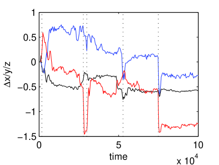
Figure 1: Non-affine displacements $\Delta x$, $\Delta y$, and $\Delta z$ (black/blue/red) for a monomer undergoing creep at $\sigma=0.5$. The vertical dotted lines indicate relaxations identified by our hop detection algorithm. The total strain during this time is approximately 0.8.

In addition to monitoring the mechanical response in the deformation protocols described above, we are interested in understanding more directly how the deformation accelerates the particle relaxation dynamics. Structural relaxations are identified on the scale of a single particle or monomer segment by monitoring a subset of five thousand particle trajectories chosen randomly from the simulation volume. Figure 1 shows an example of the non-affine particle displacement during a creep experiment (the portion of the displacement due to the macroscopic deformation of the simulation volume has been removed). The trajectories take the form of long periods of vibration where their motion is predominantly affine, punctuated by discrete hopping events.

Single particle hopping dynamics have been studied in simulations of metallic liquids and glasses Vollmayr-Lee (2004); Vollmayr-Lee and Zippelius (2005), in kinetically constrained models of supercooled liquids Hedges et al. (2007), and in experiments of colloidal glasses Chaudhuri et al. (2008) and granular materials Candelier et al. (2009), and have been very useful in understanding the nature of heterogeneous dynamics in soft glassy materials. To detect the individual hops, a running average and standard deviation is computed for the non-affine displacement of each particle over a time of $400$. The usual method of defining a hop is through a threshold in the displacement of the mean particle position, where the threshold is determined in relation to the vibrational amplitude Vollmayr-Lee (2004); Hedges et al. (2007); Chaudhuri et al. (2008); Candelier et al. (2009). However, we have observed that frequently particles experience large, intermittent fluctuations in position with little net displacement. These events can not be disregarded as hops, as the displacement is often much larger than the cage size. The ambiguity in determining a hop from a single trajectory is related to the fact that the single particle hop is only a small part of a collective relaxation event. In this work, we therefore identify hops through a threshold in the standard deviation of the displacement, rather than the mean; that is, we define relaxation events by the activity of the particle, rather than the final state. Further details of the procedure are discussed in the Appendix. Once the trajectories are reduced to a series of hops, we construct the probability distribution functions for the first hop time $p(t_{1})$ (the time from the beginning of the measurement to the first hop), the persistence time $p(\tau)$ (the time in between all subsequent hops or the residence time for a caged configuration), and the hop displacements $p(dx)$.

IV Results

IV.1 Aging at zero pressure

At finite temperature, the undeformed glass continues to evolve in a non-ergodic manner due to activated thermal processes. The non-equilibrium relaxation dynamics causes aging in all of the properties of the glass with the wait time $t_{w}$ since vitrification. The volume decreases logarithmically with the wait time, as does the potential energy. The most striking results of aging are, however, seen in the dynamical properties of the glass. Glasses obey “time-waiting time superposition”: two-time correlation and response functions can be rescaled by the wait time $C(t,t_{w})=C_{vib}(t)+C_{conf}(t/t_{w}^{\mu})$, where $\mu$ is the aging exponent and $t$ is the measurement time. Although glasses are characterized by a wide distribution of relaxation times, it appears as though they are all rescaled identically during aging.

Previously, we reported on the hop statistics in a polymer and binary metallic Lennard-Jones glass undergoing simple aging after a rapid quench Warren and Rottler (2009). Hop statistics for the polymer glass can be seen here again as solid lines in Figs. 3(b-d), and also in Figs. 5(b-d) and  6(b-d). The first hop time distributions (Fig. 3(b)) take the form of two power laws, and the intersection between the two increases with $t_{w}^{\mu}$ in the same way as the correlation and response functions. This time seems to be correlated with the cage escape time $\tau_{\alpha}$ where structural relaxations become important in the glass. Alternatively, Figure 3(c) shows that the distribution of persistence times decays as a single, age-independent power law, $p(\tau)\sim\tau^{-1.2}$. In ref. Warren and Rottler (2009), we showed that aging can be understood as the direct result of the wide distribution of persistence times which, in the thermodynamic limit, has an infinite mean. Evolving the system of particles using a continuous time random walk parameterized with the initial condition $p(t_{1},t_{w}=0)$, which reflects the quench, and the persistence time distribution $p(\tau)$ is sufficient to predict the observed changes to the first hop time distributions $p(t_{1},t_{w})$ during aging.

A power law form for $p(\tau)$ was also found for the BMLJ supercooled liquid by using a rigorous energy landscape approach to detect transitions Doliwa and Heuer (2003). Doliwa and Heuer performed frequent energy minimizations in order to detect collective relaxations in between adjacent metabasins in the potential energy landscape. The persistence time distributions were found to take the form of two power laws: at short times the transitions are continuous and liquid-like, and at long times the transitions are dominated by uncorrelated hops between metabasins. The decay at long time becomes less steep with temperature, approaching $\tau^{-2}$ as the glass transition temperature is approached from above; that is, $\langle\tau\rangle$ is finite in the liquid state. Vollmayer-Lee measured the persistence time distributions in the binary Lennard-Jones glass using a single particle hop detection algorithm which differentiates between hops that lead to an entirely new position (irreversible hops) and hops back and forth between two average positions (reversible hops) Vollmayr-Lee (2004). $p(\tau)$ was again found to decay in a weak power law ($\tau^{-0.84}$), independent of history and temperature in the glassy state.

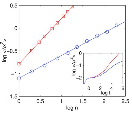
Figure 2: Mean-squared displacement as a function of the number of hops $n$ that a particle has experienced for the polymer model ($\circ$) and the BMLJ model ($\square$) (simulation details of the BMLJ results can be found in Warren and Rottler (2009)). Lines have slopes of $1/2$ (blue) and 1 (red). Inset shows the corresponding mean-squared displacement for both models with time.

Figure 3(d) shows that the hop displacement distribution $p(dx)$ also does not depend on the wait time. $p(dx)$ is sharply peaked around zero and decays rapidly at large $dx$. The rapid decay of the tails results from the connectivity of the polymer glass; the tails of $p(dx)$ are purely exponential in the binary metallic Lennard-Jones (BMLJ) glass Warren and Rottler (2009). Polymer specific dynamics is also apparent in the diffusion behaviour of the polymer glass. The mean-squared displacement $\langle\Delta x(t)^{2}\rangle$ of both the polymer model and the binary metallic Lennard-Jones glass show the two-step relaxation behaviour characteristic of glassy materials (inset Fig. 2). However, in the cage-escape regime, $\langle\Delta x(t)^{2}\rangle$ increases much more rapidly in the metallic glass than in the polymer glass. The reason for this is evident if the mean-squared displacement is plotted versus the number of hops $n$ a particle has experienced rather than the time elapsed $t$, as shown in Figure 2. The mean-squared displacement of the polymer beads increases with the number of hops as $\langle\Delta x(n)^{2}\rangle\sim\sqrt{n}$ (Rouse dynamics) rather than $\sim n$ for simple molecular glass formers due to the constraints of the covalent bonds. Alternatively, the aging behaviour of the relaxation time distributions were found to be qualitatively similar for the polymer model and the BMLJ glass Warren and Rottler (2009). This is a good indication that the results discussed here apply quite generally to glassy materials, and the polymer-specific aspects of the dynamics are seen primarily in the displacements rather than the relaxation times.

IV.2 Step stress

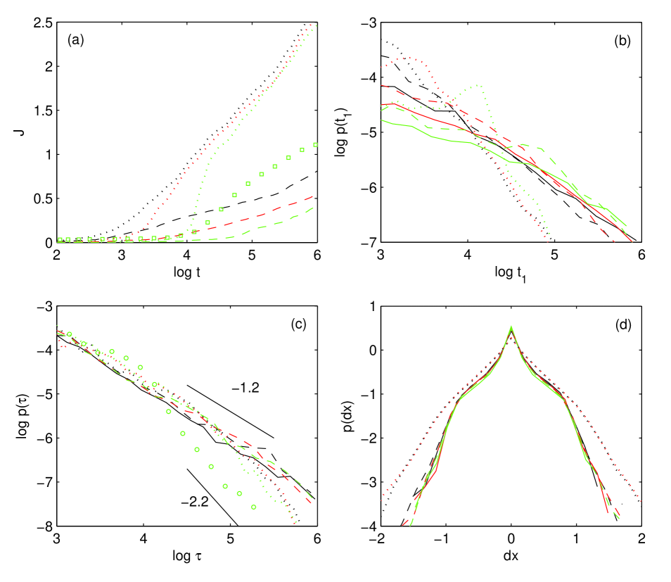
Figure 3: Relaxation dynamics during the creep experiment. (a) Creep compliance for $\sigma=0.4$ (dashed), 0.5 (dotted). Squares show the $\sigma=0.5$ curve for chains of length 100. Distributions of (b) first hop times, (c) persistence times, and (d) displacements for the undeformed sample (solid lines), $\sigma=0.4$ (dashed), and $\sigma=0.5$ (dotted). In all plots $t_{w}=750$ (black), 7500 (red), and 75000 (green). Circles in (c) show $p(\tau)$ for $t<\tau_{\alpha}\approx 10^{4}$ (see text) and $t_{w}=75000$. Straight lines indicate power law with the given slopes.

We next turn our attention to the effects of deformation on the relaxation dynamics. Figure 3 shows the mechanical response (a), and the hop statistics (b-d) in the step stress experiment. When a stress $\sigma$ is suddenly applied to the glass, the strain $\epsilon(t,t_{w})$ shows an initial elastic response followed by slow elongation, or creep, due to structural relaxations in the glass. In Figure 3(a), the creep compliance $J(t,t_{w})=\epsilon(t,t_{w})/\sigma$ is plotted as a function of wait time and stress. At small stress, the creep compliance takes the form of a stretched exponential at short times, changing to a logarithmic increase at $t\gg t_{w}$ due to the effects of aging at long times Struik (1978); Warren and Rottler (2007). For increasing wait time, the glass becomes stiffer and the creep compliance curves at short times can be superimposed to form a master curve by rescaling the time variable with a power law in $t_{w}$,

$$J(t,t_{w})=\mathcal{J}(t/t_{w}^{\mu}).$$ (1)

The aging exponent $\mu$ is approximately $0.8$ at a small stress of $\sigma=0.3$. At $\sigma=0.5$, Fig. 3(a) shows that the short time compliance depends on the wait time, but at longer times the glass yields and all history dependence is lost. The strain rate in this regime decreases over time due to the effects of strain-hardening.

The hop statistics for the $\sigma=0.4$ and 0.5 creep experiments are shown in Fig. 3(b-d), and compared to the unstressed, aging glass. For $\sigma=0.5$, the first hop times are clearly accelerated by the stress. The tails of the distribution decay with a much steeper power law than the undeformed glass ($t_{1}^{-2.2}$ vs. $t_{1}^{-1.1}$). This corresponds well to experiments, which showed that in the flow regime, not only are the segmental dynamics accelerated, but the width of the relaxation time distribution becomes narrower as well Lee et al. (2009). This distribution is narrowed for all stresses tested here, however the changes to $p(t_{1})$ are considerably smaller in the sub-yield regime. The persistence time distributions are also narrowed during the creep experiment. Unlike in the case of simple aging, $p(\tau)$ during a creep experiment depends explicitly on both the wait time $t_{w}$, and the measurement time $t$ since the stress was applied. The distributions shown in Fig. 3(c) are obtained from the persistence times of cages originating at times much greater than the cage escape time, where the strain is increasing logarithmically. The narrowing of $p(\tau)$ is even more pronounced for cages originating at shorter times (circles). This result provides an interesting explanation for mechanical rejuvenation. Since aging can be understood as the effect of an infinite mean persistence time, then aging ceases when the tails of $p(\tau)$ decay with an exponent steeper than $-2$, and a steady state is established which is independent of the age of the glass. For glasses below yield, the persistence time distribution remains in the aging regime, whereas at $\sigma=0.5$, a steady state flow regime has been established and the persistence time distribution decays with an exponent of $\sim-2.2$.

Figure 3(d) shows that the hop displacement distribution is wider for the $\sigma=0.5$ case. At this stress, $p(dx)$ depends on the strain rate (discussed further below), and is highly anisotropic. The non-affine displacements in the direction of the applied stress are significantly smaller than displacements perpendicular to the stress. This does not appear to be true at any of the smaller stresses, and is likely an effect of strain hardening during flow. The fluctuations in the direction of strain may be suppressed in this regime because the chains are extended and under tension.

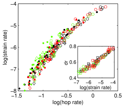
Figure 4: Strain rate versus hop rate for $\sigma=0.5$ ($\circ$), 0.4 ($\square$), 0.3 ($\triangle$), 0.2 ($\lozenge$) and $t_{w}=750$ (black), 7500 (red), and 75000 (green). Solid symbols show results for chains of length 100. Inset shows the mean hop displacement versus the strain rate for the same data.

Previous experimental Lee et al. (2008, 2009) and simulation Riggleman et al. (2007, 2008) studies have shown a strong correlation between the particle mobility and the strain rate. The mobility was defined as the inverse of a relaxation time $\tau$ obtained from the stretched exponential fits to an autocorrelation function obtained periodically throughout the creep experiment, and was found to increase almost linearly with the strain rate. The analogous quantity to the mobility in our simulations is the average hop rate, which is determined by creating a histogram of the number of hops as a function of time. A parametric plot of the strain rate versus the hop rate is shown in Fig. 4. Data for all stresses and wait times fall on a universal curve, indicating that there is a direct relationship between the macroscopic strain rate and the microscopic hopping transitions. The strain rate does not increase linearly with the hop rate, however. Even at zero stress, the hop rate is finite due to thermally activated transitions. At higher strain rates, where the hopping dynamics are highly accelerated, the strain rate increases faster than linearly with the hop rate. This can be explained by the fact that the average hop displacement also increases with the strain rate, as shown in the inset. It is possible that this is due to unresolved hops at very short times, which is discussed further below.

The polymer chains used to obtain the previous results have a length of 10 beads, which is far shorter than the entanglement length for this model. It is important to check how the results depend on chain length in our polymer model, especially at large strains where strain hardening is pronounced in entangled polymer glasses. To this end, we have performed the same simulations with chains of length 100. Figure 3(a) (squares) shows that the long-chain glass exhibits considerably more strain hardening during yield, with a lower strain and strain rate than the short-chain glass. We compare the results of the strain rate versus the hop rate for the two different chains lengths in Fig. 4. Not only does the superposition for different wait times and stresses still hold for the longer chains, but the form of the universal curve is identical to that found for the shorter chains.

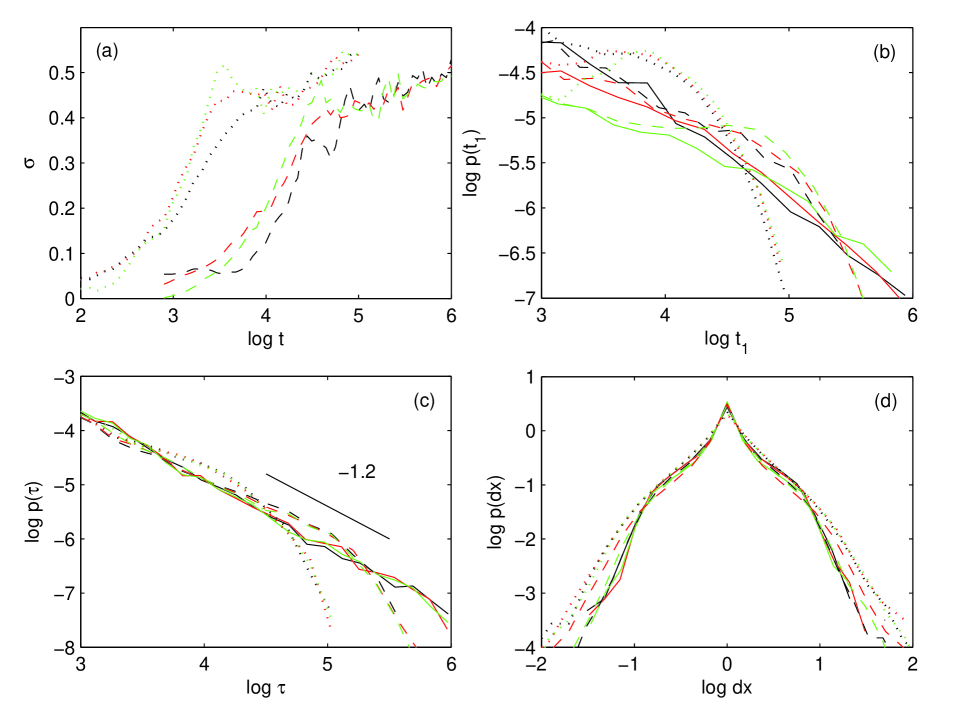
Figure 5: Relaxation dynamics during the constant strain rate experiment. (a) Stress versus time for $\dot{\epsilon}=8.9\times 10^{-7}$ (dashed) and $\dot{\epsilon}=8.9\times 10^{-6}$ (dotted). Distributions of (b) first hop times, (c) persistence times, and (d) displacements for the undeformed sample (solid lines) and $\dot{\epsilon}=8.9\times 10^{-7}$ (dashed) and $8.9\times 10^{-6}$ (dotted). In all plots $t_{w}=750$ (black), 7500 (red), and 75000 (green). Straight lines indicate power law with the given slopes.

IV.3 Constant strain rate

The stress-strain curve under constant strain rate deformation is shown in Fig. 5(a). The effects of aging appear as an increasing over-shoot stress, after which there is a period of shear softening and eventual flow. The size of this overshoot increases with the wait time, and with increasing strain rate Rottler and Robbins (2005). As in experiments Hasan and Boyce (1993), the stress on our model glass in the flow regime is independent of the wait time; all history dependence has been erased. Because of the low strain rates studied here, the stress in the flow regime is also independent of the strain rate.

The probability distributions describing the hop dynamics for this protocol are shown in Fig. 5(b-d). The constant strain rate deformation also greatly accelerates the hopping dynamics, but in a very different way than the step stress. At short times, the first hop time distributions are markedly unchanged, whereas, at long times, $p(t_{1})$ no longer decays with power law tails but is instead sharply truncated at a timescale of approximately $0.1/\dot{\epsilon}$. The same behaviour is also evident in the persistence times. In contrast with the case of the step stress, during constant strain rate flow, $p(\tau)$ does not depend on the wait time or the measurement time. This is interesting because in the flow regime strain hardening starts to become important, and yet the persistence time distribution is the same at short times and at long times. Conversely, the hop displacements are fairly isotropic at short times, and become wider and highly anisotropic during the flow regime. It would appear that strain hardening manifests in the spatial distribution of hops, rather than their relaxation times.

Mechanical rejuvenation is seen after yield in the constant strain rate protocol as well, and can similarly be explained by the persistence time distribution. The truncation in $p(\tau)$ at long times certainly means that the mean persistence time is finite and a steady state is established in the flow regime.

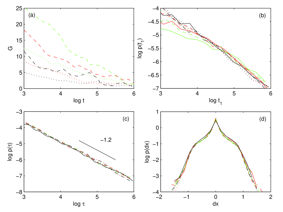
Figure 6: Relaxation dynamics during the strain step experiment. (a) Strain modulus $G=\sigma/\epsilon$ versus time for $\epsilon=0.02$ (dashed) and 0.04 (dotted). Distributions of (b) first hop times, (c) persistence times, and (d) displacements for the undeformed sample (solid lines) and $\epsilon=0.02$ (dashed) and 0.04 (dotted). In all plots $t_{w}=750$ (black), 7500 (red), and 75000 (green). Straight lines indicate power law with the given slopes.

IV.4 Step strain

The response to a step strain is defined by the modulus $G(t,t_{w})=\sigma(t,t_{w})/\epsilon$ which is shown in Fig. 6(a). Upon applying the strain, there is an immediate increase in the stress of a glass, which is larger for glasses aged for longer wait times. As the strain is held constant, the stress gradually decays due to structural relaxations over a timescale which also depends on the wait time. Like the case of the creep compliance, the step strain modulus is shifted forward in time with increasing $t_{w}$. For larger strains outside of the linear regime, $G(t,t_{w})$ decreases with increasing step strain $\epsilon$; the glass becomes softer because the dynamics are accelerated by the deformation.

The first hop time distribution (Fig. 6(b)) shows that the number of relaxations occurring at very short times is greatly increased by the step strain; however, at longer times, $p(t_{1})$ decays with the same power law as the undeformed glass. At the largest strains investigated, $p(t_{1})$ for all wait times appear to be almost identical, which would suggest a loss of history dependence (rejuvenation). The stress relaxation response indicates, however, that this is not the case. Even at very large strains, the modulus retains the features of aging. It is likely that the variation in $p(t_{1},t_{w})$ is to be found at short times where individual hops cannot be resolved by our methods. Unlike the case of both the creep and the constant strain rate experiment, the persistence times (Fig. 6(c)) and the displacements (Fig. 6(d)) are completely unaffected by the deformation: after a first hop, the particle loses all memory of the strain step. This result implies that the persistence times are not sensitive to the global stress. There is no time or wait time dependence to the persistence time distributions, even though the stress relaxation depends on both times and remains finite for the duration of the experiment. This is in direct contradiction to the Eyring model of mechanically accelerated dynamics, which says that the stress decreases transition barriers and hence increases mobility Eyring (1936).

IV.5 Acceleration Factor

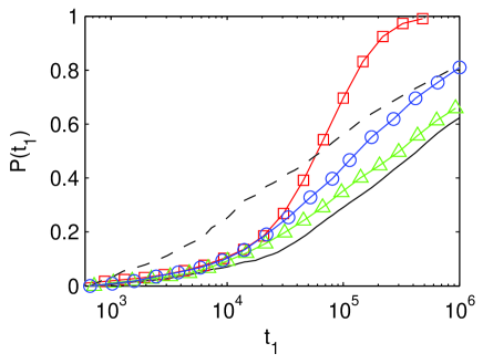
Figure 7: Cumulative probability distribution of the first relaxation event for the undeformed glass (solid line) and under deformation with a step stress $\sigma=0.3$ $(\circ)$, a step strain $\epsilon=0.01$ $(\triangle)$, and a constant strain rate $\dot{\epsilon}=8.5\times 10^{-7}$ $(\square)$ for $t_{w}=75000$. Dashed line shows the cumulative for the undeformed $t_{w}=750$ glass.

In this section, we develop a method to evaluate the complex transformations of the relaxation time distributions that were observed for the three protocols, and to determine which deformation variables best describe the accelerated dynamics. We assume that the deformed relaxation times $t_{d}$ are a function of the undeformed relaxation times $t_{u}$ as well as some undetermined parameters $\vec{p}$ which could include, for instance, the stress, strain, and/or strain rate: $t_{d}=t_{d}(t_{u},\vec{p})$. If the distribution of hop times in the undeformed case is $p_{u}(t_{u})$, then the distribution in the deformed sample becomes:

$$p_{d}(t_{d}(t_{u},\vec{p}))=p_{u}(t_{u})\frac{dt_{u}}{dt_{d}}$$ (2)

Integrating on both sides, we obtain

$$\int_{0}^{t_{d}}{p_{d}(t)dt}=\int_{0}^{t_{u}}{p_{u}(t)dt}$$ (3)

where the integrals in Eq. (3) are just the cumulative distributions $P_{u}(t_{u})$ and $P_{d}(t_{d})$ of the first hop times. The acceleration factor can therefore be defined as $t_{u}/t_{d}$, where $t_{u}$ and $t_{d}$ are the times when the undeformed and deformed cumulative distributions are equal: $P_{d}(t_{d})=P_{u}(t_{u})$. In this way, we obtain the acceleration of the entire spectrum of relaxation times during the experiment and we can determine the form of $t_{d}(t_{u},\vec{p})$, and identify the relevant parameters $\vec{p}$. This analysis can be performed on both the first hop time and the persistence time distributions.

The cumulatives of the first hop times for representatives of the three deformation protocols are shown in Fig. 7. It is clear from this figure that the acceleration factor is unique to each deformation protocol. The step strain seems to cause a simple shift in the cumulative distribution with respect to the undeformed case, which means that all relaxation times are accelerated by a constant factor. There is also experimental evidence for a simple rescaling of the relaxation times under a step strain. O’Connell et al. found that the stress relaxation after different step strains could be superimposed by shifting the curves in time, that is, the glasses obeyed “strain-time superposition” O’Connell and McKenna (2002). Alternatively, in both the stress step and the constant strain rate experiments, the cumulatives for the deformed samples continue to diverge from the reference curve at longer times. This is just another way to see that the distribution of relaxation times is narrowed: long relaxation times are accelerated more than short ones.

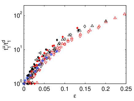
Figure 8: Acceleration factor $t_{u}/t_{d}$ as a function of global strain $\epsilon$ for three different deformation protocols. Stress step: $\sigma=0.3$ ($\circ$), 0.4 ($\square$), 0.5 ($\triangle$); constant strain rate: $\dot{\epsilon}=8.9\times 10^{-6}$ ($\lozenge$), $8.9\times 10^{-7}$ ($\triangledown$); strain step ($\triangleleft$). For each: $t_{w}=75000$ (black), 22500 (red). Also shown is the acceleration factor for the persistence times for constant strain rate deformation at $\dot{\epsilon}=8.9\times 10^{-7}$ (blue $*$). Solid symbols show results for chains of length 100.

We have already seen that the global stress is not a good variable to describe the dynamical acceleration, and the fact that the step strain causes a simple shift in $P(t_{1})$ suggests the strain as a promising alternative. In Fig. 8, the acceleration factor computed from the first hop time distribution $t_{1}^{u}/t_{1}^{d}$ is plotted parametrically versus the strain $\epsilon$ for all protocols. The acceleration factor for the three different protocols and several wait times collapse quite well onto a common curve. No similar collapse could be found for the acceleration factor versus any other macroscopic deformation variable. The acceleration factors computed using representative simulations with chains 100 beads long are also shown in Fig. 8 and have exactly the same form as the short chain results.

A strain-controlled acceleration factor also explains the observed changes to the persistence time distributions. We showed in Fig. 1 that individual particle trajectories exhibit very little non-affine displacement except during a hop. This suggests that the local strain tracks with the global strain in between relaxation events, and that the relevant parameter in analyzing the effect of deformation on the persistence times is not the total strain since the onset of deformation, but the accumulated strain in between subsequent hops. With this interpretation, we understand that the strain step causes no change to $p(\tau)$ because there is no further strain after the initial step. Note that this does not imply that there are no residual effects of the step strain on the dynamics after the first hop has relaxed the local strain: the persistence time distribution $p(\tau)$ is narrower than the first hop time distribution in an aging glass, therefore particles displaced by the deformation are more likely to hop again than those that have not. In the constant strain rate experiment, we can compute the acceleration factor of the persistence times $\tau_{u}/\tau_{d}$ from the cumulatives of $p(\tau)$ in the same way as before. Plotted versus the global strain increment in between hops (in this case, $\epsilon$ is proportional to the persistence time), Fig. 8 shows that the acceleration function for the persistence times is identical to that of the first hop times. Although it is more difficult to quantify, the dependence of $p(\tau)$ on the wait time and the measurement time in the step stress experiment can be explained by the fact that the strain explicitly depends on these same variables.

We note here that the acceleration ratios of only the longest wait time curves could be evaluated with great accuracy. Our method of identifying hops, whereby the average position and standard deviation are calculated over a time window, leads to a minimum time resolution where individual hops can be identified. The relaxation time distributions $p(t_{1})$ and $p(\tau)$ are not affected by this resolution limit, as discussed in more detail in the Appendix. However, the fact that $p(t_{1})$ and $p(\tau)$ cannot be measured at very short times does presents a problem in calculating the cumulatives, especially when there are many short time hops, such as for shorter wait times or very rapid deformations. In this case, because there are many hops at short times that are not detected, the cumulative increases abruptly from zero at the beginning of the measurement, rather than showing the smooth increase typical of the cage escape regime (see Fig. 7, dashed line). The curve is effectively shifted downward from where it should be because the integrated effect of the shortest time hops is not present. The acceleration factor is thus most accurate at long wait times, where the cumulative increases slowly from zero, and where the short time dynamics in particular are not greatly accelerated, as in the constant strain rate experiment. In the constant strain rate experiment, the acceleration factor for all wait times can be evaluated, and the curves are found to collapse. In the step strain experiment at very large strains, the short time dynamics are accelerated to such an extent that even the longest wait time sample may show truncation effects. To obtain a better estimate of the acceleration factor in this case, we additionally used curve fitting to find the factor $a$ where $p_{d}(a\times t_{1})/a$ most closely resembled $p_{u}(t_{1})$ and vice versa, fitting $a\times p_{u}(t_{1}/a)$ to $p_{d}(t_{1})$. The short time resolution of our technique may also be the cause of the widening displacement distributions with strain rate. If several hops occur within our minimum resolution, they are detected as a single hop, possibly with a wider displacement. It is unclear from our results to what extent the elementary hop displacements actually grow with the strain rate.

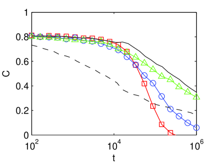
Figure 9: Incoherent scattering function $C(t,t_{w})$ with $|\mathbf{q}|=7.0$ averaged over the non-deformed ($y$ and $z$) directions for the undeformed glass (solid line) and under deformation with a step stress $\sigma=0.3$ $(\circ)$, a step strain $\epsilon=0.01$ $(\triangle)$, and a constant strain rate $\dot{\epsilon}=8.5\times 10^{-7}$ $(\square)$ for $t_{w}=75000$. Dashed line shows $C(t,t_{w})$ for the undeformed $t_{w}=750$ glass.

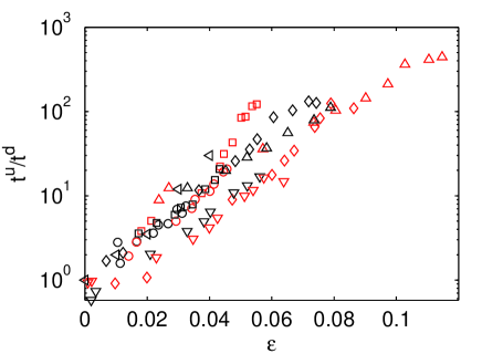
Figure 10: Acceleration factor calculated from the incoherent scattering function as a function of global strain $\epsilon$ for three different deformation protocols. Stress step: $\sigma=0.3$ ($\circ$), 0.4 ($\square$), 0.5 ($\triangle$); constant strain rate: $\dot{\epsilon}=8.9\times 10^{-6}$ ($\lozenge$), $8.9\times 10^{-7}$ ($\triangledown$); strain step ($\triangleleft$). For each: $t_{w}=75000$ (black), 7500 (red).

The hop statistics provide a powerful way of evaluating the full relaxation time distributions and their history dependence. Unfortunately, the first hop time and persistence time distributions are probably not directly accessible in real polymer glasses. However, it may be possible to calculate the acceleration factor from the autocorrelation functions more typically used to measure glassy dynamics. In Fig. 9, we plot the intermediate scattering function $C(t,t_{w})=\langle\exp[-i\mathbf{q}\cdot(\mathbf{r}(t,t_{w})-\mathbf{r}(0,t_{w}))]\rangle$ under the same deformation conditions as the cumulatives in Fig. 7. Once again the affine portion of the deformation is removed and, to minimize the effect of possible strain hardening, $C$ is calculated only in directions perpendicular to the direction of strain. It can be seen that these curves are qualitatively similar to $1-P(t_{1})$. This close connection is to be expected: $1-P(t_{1})$ measures the number of particles that have not yet hopped by time $t_{1}$, which is another measure of the particle autocorrelation. The intermediate scattering function additionally includes the effects of multiple hops, since each hop need not be very large. This effect causes a steeper decay in $C(t,t_{w})$ than in $1-P(t_{1})$, especially when the subsequent hops are also accelerated. An acceleration factor $t^{u}/t^{d}$ can be defined for the scattering function decay in the same way as for the cumulatives through the relationship $C_{u}(t^{u})=C_{d}(t^{d})$, where $C_{u}$ and $C_{d}$ are the undeformed and deformed correlation functions respectively. This acceleration factor is shown in Fig. 10, and also approximately collapses as a function of the strain. The curves increase nearly exponentially for all strains, and more rapidly than the acceleration function calculated from the first hop time distributions. The scatter in this plot is significantly higher than for the acceleration factor calculated from the cumulative distributions, for reasons that are not entirely understood. However, we believe this measure holds promise for confirming experimentally whether the strain is indeed a good way to describe deformation-induced acceleration of the relaxation dynamics in glasses. Our analysis evaluates the full shape change of the particle auto-correlation function due to deformation, rather than reducing the data to an average mobility and width of the correlation decay.

V Discussion and Conclusions

The statistics of single particle hopping dynamics have been evaluated under three different deformation protocols. All three deformation modes accelerate the segmental dynamics, although the exact transformation of the relaxation time distributions is specific to the mode of deformation. The universal collapse observed in Fig. 8 of the acceleration factor as a function of the strain is strong evidence that the local strain is a good variable to describe the influence of deformation on structural relaxations, rather than the global stress as postulated by the Eyring model. A compelling reason for this is suggested by the behaviour of the stress and strain at a local level. While the local strains track very well with the global strain in between relaxation events, the global stress does not predict the evolution of stress on a coarse-grained scale Yoshimoto et al. (2004). The local distributions of moduli and stress surely account for the wide distribution of relaxation times Tsamados et al. (2009), however the strain appears to be a better predictor of how these relaxation times are accelerated.

By tracking the individual particle relaxations, our analysis permits direct observation of the narrowing of the relaxation time spectrum during creep and constant strain rate deformation, which previously was inferred only indirectly from stretched exponential fits to correlation functions Lee et al. (2009). The strain-controlled acceleration factor also provides a simple, intuitive explanation for the narrowing: particles with long relaxation times experience more acceleration than particles that hop sooner simply because they experience more strain in the long period of time in between relaxations. Alternatively, a step strain leads to a simple shift in the first hop times (no narrowing), and no change at all to the persistence times. The fact that the persistence times are unchanged in the step strain protocol suggests that the strain at the microscopic level is released after a relaxation event, or reset to zero. This interpretation is further confirmed by the fact that the acceleration of the persistence times for the constant strain rate experiment is identical to that found for the first hop times if, instead of the total strain, the strain in between subsequent hops is taken to be the relevant mechanical parameter.

Our results do not imply that the average segmental dynamics in the glass should be monotonically increased with the strain. In their experiments measuring the segmental dynamics during creep at stresses above yield, Lee et al. found that the average segmental mobility increases with strain at first, becoming a maximum where the strain rate was largest, and then decreases again in the strain hardening regime Lee et al. (2009). This is completely consistent with the strain-controlled acceleration factor presented here. The acceleration factor increases with the strain only in between subsequent hops; as discussed previously, after a relaxation event the local “strain clock” is reset to zero. As a result, at the beginning of a deformation experiment, the local strains track closely with the global strain; however, after some time, the local strains in the glass become spatially heterogeneous, being higher in regions that have not yet relaxed, and lower in regions that have recently experienced a relaxation. In the steady state flow regime, our simulations show that every particle has hopped at least once and usually many times. The advantage of molecular dynamics simulations is that the individual trajectories reveal exactly how much time has elapsed between local relaxations and thus how much strain has accumulated in each local region.

It is interesting to note that the strain was chosen as control variable in the Soft Glassy Rheology (SGR) model Fielding et al. (2000). Here the acceleration factor for barrier crossings increases proportional to $\exp[kl^{2}/2x]$, where $k$ is the elastic constant of a mesoscopic element, $l$ a measure of local strain on that element and $x$ denotes a noise temperature. The local strains increase in tandem with the global strain in between barrier crossings, and after a hop, the mesoscopic element returns to a position of zero local strain. The main elements of the SGR model closely resemble our findings for the single particle relaxation times. The measured form of the acceleration factor is, however, quite different. It would be interesting to see if using the measured form of the acceleration factor could account for some of the limitations identified in this model Warren and Rottler (2008).

The hop statistics under deformation also present an explanation for mechanical rejuvenation. In contrast to the case of sub-yield deformations where the response continues to show explicit history dependence, the effects of aging are lost once the glass has yielded. Non-stationary dynamics occurs in glasses because of the wide distribution of persistence times. An infinite $\langle\tau\rangle$ means that an equilibrium state is impossible, and the dynamics experiences aging. During yield in both the step stress and the constant strain rate protocols, the persistence time distributions are significantly narrowed, and stationary dynamics are restored. The resulting rejuvenated state is, however, not the same as a just-quenched glass. The relaxation time distributions depend explicitly on the deformation protocol. Further investigation of the relaxation time distributions after deformation may shed more light on the nature of the rejuvenated state.

The hop dynamics under deformation also provide some information about strain hardening in polymer glasses. We have tested two different chain lengths and find that the hop rate versus strain rate and the acceleration versus strain are identical for both chain lengths. Even though strain hardening is significantly more pronounced in the long-chain glass, the deformation appears to affect the hop dynamics in the same way. Strain hardening is most evident in the displacement distribution, which becomes anisotropic and significantly narrower in the strain direction. Further study of the hop dynamics during strain hardening may provide further insight into this very important behaviour of polymer glasses.

In conclusion, by detecting individual segmental relaxations, the full transformation of the relaxation time distributions under deformation could be quantified and correlated with the global deformation parameters in a model polymer glass. We find that the accelerated segmental dynamics are fully explained by the global strain, and we present a possible experimental test of these findings though the definition of the acceleration factor for any segmental autocorrelation function such as the incoherent scattering function.

*

Appendix A Identifying hopping events

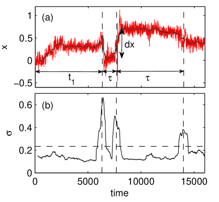
Figure 11: (a) A typical particle trajectory in the glass. Red curve shows raw position data in the x-direction, and the black curve shows the running average. (b) Standard deviation in the three dimensional particle position over the averaging window. Hops are identified by a threshold in the standard deviation, shown here as a horizontal dashed line, and marked in both frames as vertical dashed lines. In panel (a) the first hop time, persistence times, and particle displacements are also labeled.

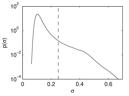
Figure 12: Probability distribution of the standard deviation $\sigma$ in the particle position over an averaging time window of 400 for all particle trajectories. Dashed line shows the threshold $\sigma_{th}$ for detecting a hop.

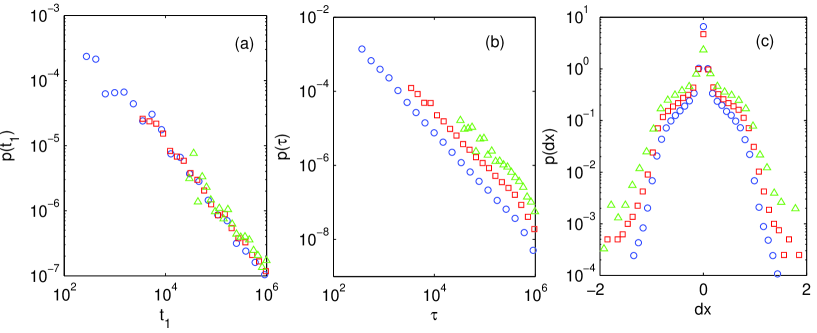
Figure 13: The distributions (a) $p(t_{1})$, (b) $p(\tau)$ and (c) $p(dx)$ for $t_{dump}=3.75$ (circle), 37.5 (square) and 375 (triangle).

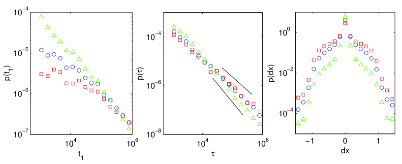
Figure 14: The distributions (a) $p(t_{1})$, (b) $p(\tau)$ and (c) $p(dx)$ for $\sigma_{th}=0.15$ (square), 0.25 (circle), and 0.35 (triangle). Solid lines in (c) indicate power laws with slope of -1.5 and -1.1.

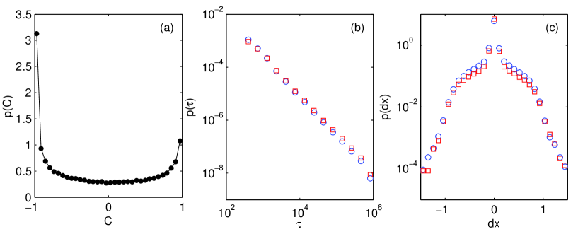
Figure 15: (a) The distribution of hop correlations, (b) $p(\tau)$, and (c) $p(dx)$ computed with all of the hops detected (circles), and with only uncorrelated hops (squares).

Particle positions are written to file with a period of $t_{dump}$. The trajectories show rapid vibrations about a mean position, punctuated by the occasional hop to a new location. To detect the hopping transitions, the average and standard deviation of each particle position is computed over $N_{avg}$ snapshots at times $t_{i}=N_{avg}\times t_{dump}\times(i-1/2)$. The trajectories and standard deviation are shown in Fig. 11. The value of $N_{avg}$ used for determining the mean and standard deviation is on the order of $40-60$ snapshots for the work presented here. Increasing $N_{avg}$ by a factor of 10 (from 40 to 400), causes negligible changes to the hop statistics but seriously decreases the time resolution of the distributions. The criteria for finding a hop is that the standard deviation of the particle position over $N_{avg}$ snapshots is greater than a threshold: $\sigma>\sigma_{th}$. To choose a suitable threshold, we look at the distribution of the standard deviations over the full time series of all of the particles in the system (see Fig. 12). There are clearly two regimes of motion in $p(\sigma)$: a narrow vibrational regime and a hopping regime. $\sigma_{th}$ is chosen to be at the shoulder in between these regimes and is shown in Fig. 12 as a dashed line. The effects of the threshold on the distributions is discussed below.

The times at which a hop occurs are determined by the centre of the standard deviation peak, and the displacements are found from the positions on either side of the peak. The distribution of displacements is easily computed by binning the data to form a histogram. Because the relaxation time distributions are very broad, the bin sizes for $p(t_{1})$ and $p(\tau)$ increase logarithmically with time in order to obtain good statistics. The finite timespan of the simulation means that this distribution is necessarily truncated. In other words, some of the particles will not have hopped at all during the experiment. For the first hop times $t_{1}$, this can be accounted for by normalizing to the total number of particles in the ensemble, rather than the number of first hops detected. The persistence time $\tau$ is defined as the time in between all subsequent hops. Accounting for the effects of truncation on this distribution is somewhat more complex than in the case of $p(t_{1})$. If all of the hops are assembled into a single distribution function as described above, there is a sharp downturn in $p(\tau)$ near the maximum time observed $t_{max}$. The distribution of persistence times that we observe $p_{obs}(\tau)$ is weighted by the probability that we will observe it within $t<t_{max}$, which becomes low for cages originating near the end of the simulation time. This effect can be accounted for using multiple convolutions of the relaxation time distributions; however since the downturn is very sharp, it is in practice easier to simply discard the very long time data.

The effect of the dump frequency on the distributions was investigated by recording the same data at three different values of $t_{dump}$. Figure 13 shows the effect of $t_{dump}$ on (a) $p(t_{1})$, (b) $p(\tau)$ and (c) $p(dx)$. Changing $t_{dump}$ does not affect the first hop time distribution $p(t_{1})$, aside from the obvious relationship between $t_{dump}$ and the minimum $t_{1}$ that can be observed. Distributions recorded at different values of $t_{dump}$ are in perfect agreement where their time spans overlap. The persistence time distribution $p(\tau)$ has the same slope for all values of $t_{dump}$, however the curves differ by a normalization factor which depends on the minimum time resolution in $\tau$. An absolute normalization factor may be obtained by using a similar method to that used to normalize the distributions $p(t_{1})$: the time between the first and second hops are found for a subset of $N$ particles where $t_{1}$ is very short. Not all of these particles will experience a second hop, and if the distribution is normalized to $N$ rather than the number of second hops, a normalized distribution is obtained that does not depend on $t_{dump}$. This method requires throwing away most of the persistence time data, however, and is therefore only used to properly normalize the full distribution which includes all measured persistence times. The displacement distribution $p(dx)$ becomes somewhat wider with increased $t_{dump}$ due to the effects of undetected hops on timescales shorter than $t_{dump}$. The distributions compared here have identical $t_{dump}$.

The effect of the threshold on the standard deviation was also investigated using three different values: $\sigma_{th}=0.15$, 0.25, and 0.35. The distributions computed using these thresholds are compared in Figure 14. Changing the threshold results in quantitative, rather than qualitative changes to the distributions. In all cases, the hop time distributions take the form of power laws, although the exponent is modified by the threshold (from about -1.1 to -1.5 for $p(\tau)$), and the first hop time distribution depends on $t_{w}$ whereas the persistence time distribution does not. However, if the threshold is very small, the influence of wait time is decreased because of noise (vibrations rather than hops) that does not depend on $t_{w}$; if $\sigma_{th}$ is very large, the statistics become poor and many legitimate hops are discarded. The hop displacements predictably become larger with increasing threshold. Using a continuous time random walk Warren and Rottler (2009), we find that the mean squared displacement and van Hove function are self-consistently described by the hop statistics obtained using a range of thresholds near the shoulder of $p(\sigma)$ (Fig. 12).

In order to model the trajectories as a continuous time random walk we assume that the hops are completely uncorrelated. To ensure that this is a reasonable approximation, the correlations between adjacent hops in the trajectories are evaluated. A correlation function can be defined for each pair of displacement vectors $\mathbf{r}_{i}$

$$C_{i}=\frac{\mathbf{r}_{i+1}\cdot\mathbf{r}_{i}}{\left\|\mathbf{r}_{i+1}\right\|\left\|\mathbf{r}_{i}\right\|}.$$ (4)

The distribution of these correlations are evaluated for all pairs of hops, as shown in Fig. 15(a). A completely uncorrelated random walk would have a flat distribution; however, we see that there are a number of backward correlated ($C=-1$) and forward correlated ($C=1$) hops. If these hops are removed from the time series data and the distribution of persistence times and displacements are computed with only the uncorrelated hops, we see no appreciable difference in the hop statistics (Fig. 15(b) and (c)).