Metal-insulator transition in hydrogenated graphene as manifestation of quasiparticle spectrum rearrangement of anomalous type

Abstract

We demonstrate that the spectrum rearrangement can be considered as a precursor and a basis for the metal-insulator transition observed in graphene dosed with hydrogen atoms. The Anderson-type transition is attributed to the Fermi level’s entering into the quasigap, which develop in the vicinity of the impurity resonance energy due to the anomalous spectrum rearrangement. Theoretical results for the Lifshitz impurity model are in a reasonable agreement with available experimental data.

I introduction

Since the existence of Dirac quasiparticles has been proved for graphene, one of the most intriguing issues of its physics is the possibility of their localization by whichever imperfection that can appear in the honeycomb lattice.castr ; beena ; altsh ; gorba ; chang ; bardas Moreover, It should not be overlooked that the effect of disorder on the transport of quasiparticles is sensitive to the nature of inhomogeneity, be it caused by short-range or long-range defects, neutral or charged impurities, adsorbed or interstitial atoms or molecules, vacancies, spatial distortions or structural irregularities, including ripples on the graphene sheet and other long-wave random modulations. All these different types of imperfections necessitate corresponding dedicated studies, which can not be accomplished by resorting to a single impurity model. Since these imperfections are rather dissimilar both in their character and action on basic properties of graphene, respective theoretical models should be diverse as well.

Early experiments on graphene-based devices, which were engineered like a commonplace field effect transistors, revealed that the sample conductivity never drops below a certain minimal value.natur This fact, indeed, considerably reduced audacious expectations that corresponding devices are capable to serve as next-generation electronic switches. Nevertheless (or, maybe, exactly because of this), the minimal conductivity existence has produced quite a stir, and its origin has been relentlessly debated. Distinctive features of charge carriers, which were shown to obey the linear dispersion, constituted the core of this discussion. Uniqueness of the electron subsystem in graphene were pushed to its limits so much that former physics of semiconductors were sometimes categorically declared being utterly unsuitable for this uncommon material. It has been speculated that massless, according to their Dirac dispersion, charge carriers can not be localized by any degree of disorder caused by lattice imperfections or impurity centers. The presumed impossibility to localize Dirac excitations were directly linked to the minimal conductivity phenomenon by a simple reasoning. Since the product of the wave vector modulus and the mean free path is confined from below for propagating states according to the Ioffe-Regel criterion, the conventional Drude expression immediately yields the minimum value of $\sim e^{2}/h$ for each conducting channel. This argument, along with available experimental results, has led to an opinion that the minimum conductivity value has a universal character for graphene, and is expressed only through fundamental constants.

In the mean time, there appeared occasional theoretical studies, which did not deny a possibility to localize charge carriers in graphene, and argued for the mobility edge appearance under certain circumstances, either for a disorder of a general type,alein ; mirli or for a specific impurity model, in particular, for substitutional defects,naumi and for the Anderson model of disorder.amini ; roche ; feng Later, it has become apparent that the minimal conductivity in graphene does depend on the sample quality and noticeably varies with the impurity concentration.fuhre ; mucci ; peres ; sarma ; ugart Furthermore, not so long ago, a metal-insulator transition (MIT) in graphene dosed with atomic, which is essential, hydrogen has been convincingly observed. The MIT has been manifested by an increase of the room temperature resistance in about four orders of magnitude.roten The transition has been reported for the grown on SiC surface graphene with a low hydrogen coverage, namely, around $0.1\%$. The presence of the mobility gap has been also reported for the fluorinated and ion bombarded graphene.savch ; ionir

As well, corresponding data of ARPES measurements indicated the disappearance of quasiparticle excitations in the system. The MIT of the Anderson type comes about when the Fermi level finds itself inside a domain of localized states. Since the graphene in the actual experiment was pristine before the hydrogen deposition and possessed sounding metallic properties with conventional Fermi-liquid behavior, it is tempting to anticipate that some amount of deposited hydrogen is sufficient to open up a reasonably wide region filled with localized states, or a quasigap, in the spectrum. In essence, this draft description of the leading to the MIT process corresponds to the well-known phenomenon of spectrum rearrangement,ivlpo ; lifsh which deals with decisive modifications in the elementary excitation spectrum upon increasing the impurity concentration in the system. When the quasigap is located in the vicinity of the Fermi level position, the MIT can take place in spite of the rather low hydrogen concentration. Below we are going to link together the predicted spectrum rearrangement in graphene with point defects and the observed MIT under the hydrogen dosing.roten The spectrum rearrangement takes place when a single impurity induces a local or a resonance level in the spectrum. It has been demonstrated recently that graphene almost inevitably contains traces of impurity centers, which are capable in producing resonance states.nov

II Criticality and types of spectrum rearrangement

Let us discuss some general spectral properties of impure systems and assume for this purpose that inside an isolated host band in a hypothetical $d$-dimensional system a single impurity center accounts for a resonance state with the energy $\varepsilon_{r}>0$, which is measured against the band edge and has been made dimensionless by the corresponding bandwidth. The dispersion relation for this host band is supposed to be of the form $\varepsilon(\bm{k})\sim k^{p}$. Then, the spatial behavior of the host Green’s function at a given energy inside the band, apart from any other details, should be governed by oscillations with the characteristic radius $r\sim\varepsilon^{-1/p}$, which is expressed in units of the appropriate lattice constant. At the energy $\varepsilon_{r}$, these oscillations determine the effective radius $r_{im}\sim\varepsilon_{r}^{-1/p}$ of the impurity state. Through a closeness of the resonance energy to the band edge, the effective radius of the impurity state may far exceed the lattice period. As the impurity concentration is increased, the individual impurity states are becoming more tightly packed. It can be anticipated that a significant spatial overlap between these states is capable in provoking qualitative changes in the spectrum. The average distance between impurities $\bar{r}\sim c^{-1/d}$, where $c$ is the (relative) impurity concentration, is gradually shrinking with increasing $c$, and at some stage of the process becomes of the order of $r_{im}$. This general condition defines the critical concentration $c_{SR}\sim\varepsilon_{r}^{d/p}$ of the spectrum rearrangement in the corresponding impure system. It seems justifiable to reiterate here that the value of $c_{SR}$ can be fairly low due to the smallness of the energy $\varepsilon_{r}$.

Graphene is, evidently, a two-dimensional system, so that $d=2$, and features the linear dispersion of charge carriers, which implies that $p=1$. Consequently, the critical concentration of spectrum rearrangement in the impure graphene is expected to be $\sim\varepsilon_{r}^{2}$, where energy is counted from the Dirac point, at which the valence band and the conduction band coincide. In a case of the conventional dispersion with $p=2$, the identical in appearance relation between $\varepsilon_{r}$ and $c_{SR}$ is inherent in four-dimensional systems. In this sense graphene, as regards the spectrum rearrangement, can be formally viewed as a conventional system of increased spatial dimensionality. This fact further accentuates the uniqueness of graphene, since the spectrum rearrangement has not been studied for such systems.

Let us return back to experimental data contained in Ref. roten, . The comparison of angle-integrated spectrum for clean and hydrogen dosed graphene suggests that the dimensional resonance energy $E_{r}$ lies somewhere around $0.25$ eV lover than the initial Fermi level, while the Dirac point position $E_{D}$ in the undoped crystal is about $0.45$ eV below it. A bit more careful analysis of the spectrum rearrangement in impure graphene, skrlo which is based on the expansion of the self-energy into a cluster series,ivlpo brings about the following expression for $c_{SR}$, which, for a convenience, is rewritten here in terms of the hydrogen coverage,

$$n_{SR}\sim n_{C}\frac{(E_{r}-E_{D})^{2}}{W^{2}},$$ (1)

where

$$n_{C}=\frac{4}{\sqrt{3}a^{2}}\approx 3.8\times 10^{15}\textrm{cm}^{-2}$$ (2)

is the areal density of carbon atoms in graphene, $a=0.246$ nm – the lattice constant of graphene, $n_{SR}$ – the critical coverage of hydrogen atoms, $W\approx 6.3$ eV – the bandwidth parameter, and the logarithmic correction is omitted because of the relatively large resonance energy. Substitution of the guessed value for the resonance energy results in $n_{SR}$ that is reasonably close to the reported MIT critical hydrogen coverage of $3.8\times 10^{12}$ cm^-2.roten As a matter of fact, the critical coverage of the spectrum rearrangement $n_{SR}$, should not be identical to the experimentally obtained hydrogen coverage required for the MIT, which will be discussed later.

It should be also noted that there are two main types of the spectrum rearrangement: the cross one, which is usually accompanied by a sharp single impurity resonance, and the anomalous one. The first type of the spectrum rearrangement results in a quasiparticle dispersion that looks like a familiar hybridization between the host branch and a dispersionless branch at the impurity resonance energy. In this case, two new branches are separated by a gap, which widens with an increase in the impurity concentration. Consequently, two different wave vectors correspond to the same energy in this split spectrum. However, this feature has not been detected in the ARPES measurements on the hydrogenated graphene. The second type of the spectrum rearrangement, which is usually encountered in low-dimensional systems, is of a more diffused nature and frequently corresponds to a considerably smeared single impurity resonance. This anomalous spectrum rearrangement is characterized by the opening of the quasigap, which is filled with localized states and separates two non-overlapping branches of extended states exhibiting a renormalized dispersion.

III Interplay between spectrum rearrangement and Anderson transition

The anomalous type of the spectrum rearrangement has been shown to unfold in graphene for impurities described by the Lifshitz model.skrlo Within this model, identical impurity centers are supposed to be randomly distributed on sites of the host lattice. Each impurity is only allowed to change the on-site energy at its location in the corresponding tight-binding Hamiltonian. It is well-known that the electron subsystem in graphene encompasses practically free $\pi$-electrons, which number is equal to the number of lattice sites. As soon as an additional hydrogen atom lands on graphene, its uncoupled s-electron immediately enters a chemical bond with one of the $\pi$-electrons. That should make the latter one localized almost completely at the impurity site. In the first approximation, one can assume that the resulting perturbation comes only from the appearance of strong attracting potential on the occupied carbon atom. Thus, the disordered system is described by following operators,

$$\bm{H}=\bm{H}_{0}+\bm{H}_{im},\qquad\bm{H}_{im}=V_{L}\sum\limits_{\bm{n}\alpha}\eta_{\bm{n}\alpha}^{\phantom{\dagger}}c_{\bm{n}\alpha}^{\dagger}c_{\bm{n}\alpha}^{\phantom{\dagger}},$$ (3)

where

$$\bm{H}_{0}=t\sum\limits_{\bm{n}\alpha,\bm{m}\beta}c_{\mathbf{n}\alpha}^{\dagger}c_{\mathbf{m}\beta}^{\phantom{\dagger}}$$ (4)

is the host Hamiltonian, in which summation is restricted to nearest neighbors, $\bm{n}$ runs over lattice cells, indices $\alpha$ and $\beta$ enumerate sublattices, $c_{\bm{n}\alpha}^{\dagger}$ and $c_{\bm{n}\alpha}^{\phantom{\dagger}}$ are the creation and annihilation operators at the corresponding lattice site, $t\approx 2.7$ eV – is the tight-binding transfer integral for the $\pi$ bands in graphene, the variable $\eta_{\mathbf{n}\alpha}$ takes the value of $1$ with the probability $n_{H}/n_{C}$ or the value of $0$ with the probability $1-n_{H}/n_{C}$, where $n_{H}$ is the hydrogen coverage, and $V_{L}<0$ is the difference in the on-site potential at the defect position.

Within this model, the local density of states (LDOS) at the lattice site occupied by a hydrogen reads,

$$\rho_{im}(E)=-\frac{1}{\pi}\operatorname{Im}\frac{g_{0}(E)}{1-V_{L}g_{0}(E)},$$ (5)

where $g_{0}(E)$ is the diagonal element of the host Green’s function

$$\bm{g}=(E-\bm{H}_{0})^{-1}.$$ (6)

In the vicinity of the Dirac point in the spectrum, namely, within the window stretching up to around $0.75$ eV to each side of it, this diagonal element can be easily approximated,

$$g_{0}(E)\approx\frac{E-E_{D}}{W^{2}}\ln\left(\frac{E-E_{D}}{W}\right)^{2}-i\pi\frac{|E-E_{D}|}{W^{2}},$$ (7)

where

$$W=\sqrt{\pi\sqrt{3}}t$$ (8)

is the same bandwidth parameter as in (1). Substitution of this approximation to Eq. (5) yields

$$\rho_{im}(E)\approx\frac{|\mathcal{E}|}{W[(1-2\frac{V_{L}\mathcal{E}}{W}\ln|\mathcal{E}|)^{2}+(\pi\frac{V_{L}\mathcal{E}}{W})^{2}]},$$ (9)

where

$$\mathcal{E}=(E-E_{D})/{W}.$$ (10)

The LDOS at the impurity site is shown in Fig. 1 for $V_{L}=-25$ eV. As follows from the Figure, the resonance energy $E_{r}$ is located approximately $0.2$ eV above the Dirac point and thus corresponds to the experimentally observed peak. While the required change in the on-site potential is quite substantial, the large perturbation magnitude should be considered, first of all, as a result of the chosen simplified impurity model. Unless another is explicitly specified, the perturbation value of $-25$ eV will be used below for all subsequent estimations.

Figure 1: Local density of states at the impurity site for $V_{L}=-25$ eV.

When a certain amount of deposited hydrogen atoms is taken into account, the negative potentials induced by them on the occupied lattice sites impede the electron movement. For the Lifshitz impurity model, which has been described above, the course of the spectrum rearrangement has been studied both analytically and numerically.skrlo ; persk The analysis has shown that states are subject to localization near the resonance energy, where the impurity scattering is the strongest. At some coverage, a quasigap occupied by localized states opens around the energy $E_{r}$. With increasing impurity concentration, the quasigap gradually broadens and the degree of localization inside it rises. This quasigap expansion and the localization enhancement are not symmetric about the energy $E_{r}$ and are more expressed above the resonance (for an attractive potential). Finally, the quasigap consumes all the space between $E_{r}$ and $E_{D}$ in the spectrum, which corresponds to the onset of the spectrum rearrangement by the definition. In other words, the spectrum rearrangement does follow the anomalous scenario.

In the experiment discussed, dosed hydrogen atoms act not only as scattering centers, but also as acceptors. Thus, their presence inevitably lowers the Fermi level of the system. Therefore, while the hydrogen coverage is increasing, the Fermi level and the upper boundary of the quasigap, where the localization of states is most pronounced, are moving toward each other. Sooner or later, the Fermi level should appear inside the quasigap, which will cause the MIT of the Anderson type. Since the energy $E_{r}$ is positioned somewhere in-between $E_{D}$ and the bare Fermi level $E^{(bare)}_{F}$, the critical coverage of the spectrum rearrangement should be close but not identical to the critical coverage of the MIT.

The acceptor effect of the deposited hydrogen atoms is also implicitly contained in the Lifshitz model. Strong attracting potential $V_{L}<0$ produces a deep local level below the conduction band. Because of its remoteness from the continuous spectrum, the corresponding narrow impurity band should hold almost $n_{H}N_{C}/(2n_{C})$ energy levels, where $N_{C}$ is the total amount of carbon atoms in the system. Thus, taking into account the spin degeneracy, this impurity band consumes nearly one electron per deposited hydrogen atom. However, apart from these qualitative considerations, the adopted impurity model allows to address the question on the Fermi level position more precisely. Consider the (normalized) total number of states with energies that are less than a specified one,

$$N(E)=\int_{-\infty}^{E}\rho(E)\,\mathrm{d}E,$$ (11)

where $\rho(E)$ is the density of states. In a disordered system this quantity can be expanded in powers of the impurity concentration,lifsh

$$N(E)=N_{0}(E)+\frac{2n_{H}}{\pi n_{C}}\arg(1-V_{L}g_{0}(E))+\dots,$$ (12)

where the presence of two sublattices in graphene and the Lifshitz impurity model are taken into account, and $N_{0}(E)$ is the total number of states in the host system. Keeping in mind that the deep impurity band is modeling the acceptor effect of impurities, it is natural to demand the conservation of the number of occupied states in the system with varying the amount of dosed hydrogen. This yields a kind of a balance condition,

$$\operatorname{sgn}\left(\frac{E_{F}-E_{D}}{W}\right)\frac{(E_{F}-E_{D})^{2}}{W^{2}}+\frac{2n_{H}}{\pi n_{C}}\arg(1-V_{L}g_{0}(E_{F}))=\frac{(E^{(bare)}_{F}-E_{D})^{2}}{W^{2}},$$ (13)

where the constant term is dropped from the both sides of the equation, and Eq. (7) is used to obtain $N_{0}(E)$ for the clean graphene. From here and on this condition will be employed to determine the Fermi level position at a given dosing level. It is worth mentioning that the Dirac point position (which should not be confused with its value for the unperturbed system $E_{D}$) is gradually shifted with increasing the impurity concentration by approximately $n_{H}V_{L}/n_{C}$. Since the Dirac point and the Fermi level are both moving in one direction, namely to lower energies, the distance between them does not shorten remarkably.

IV Conduction band spectrum

For $n_{H}<n_{SR}$, the presence of attracting impurities does not distort significantly the quasiparticle dispersion in the valence band. In contrast, impurities noticeably affect the conduction band. The self-energy $\bm{\Sigma}$, which enters the Dyson equation

$$\bm{G}=\bm{g}+\bm{g}\bm{\Sigma}\bm{G}$$ (14)

for the averaged over impurity distributions Green’s function of the disordered system

$$\bm{G}=\biglb<(E-\bm{H})^{-1}\bigrb>$$ (15)

can not be attributed only to the impurity scattering in the actual experiment of Ref. roten, , because the linewidth of the ARPES data is not negligible even at the absence of impurities. To deal with this issue, we assume that all other sources of its broadening, except the controlled amount of hydrogen atoms, can be roughly described by a constant dumping term,

$$\bm{\Sigma}\approx\bm{\Sigma}_{im}-i\Gamma\bm{I},\qquad\Gamma>0,$$ (16)

where $\bm{\Sigma_{im}}$ is those part of the self-energy, which results from the impurity scattering, and $\bm{I}$ is the identity matrix. A comparison of the density of states obtained by the numerical simulation with the one resulted from the standard average T-matrix method showed that at $n_{H}<n_{SR}$ this approximation works rather well in the vicinity of the impurity resonance.persk Within this single-site approximation, the impurity-induced part of the self-energy is diagonal in lattice sites and sublattices for point defects,

$$\bm{\Sigma}_{im}\approx\frac{\frac{n_{H}}{n_{C}}V_{L}}{1-(1-\frac{n_{H}}{n_{C}})V_{L}g_{0}(E)}\bm{I}.$$ (17)

Thus, taking into account both assumptions, the total self-energy is also diagonal,

$$\bm{\Sigma}\approx\Sigma(E)\bm{I}.$$ (18)

According to the conventional expression for the spectral function,

$$A(E,\bm{k})\approx-\frac{1}{\pi}\operatorname{Im}\frac{1}{E-\Sigma(E)-v_{F}k},$$ (19)

where

$$v_{F}=\frac{\sqrt{3}at}{2}$$ (20)

is the Fermi velocity, the wave vector $\bm{k}$ is counted from the corresponding Dirac point, and only one branch, which is manifested in the actual experiment, is retained, it is straightforward to put down corresponding expressions for the inverse width of the momentum distribution curve at its half-height,

$$L(E)\approx-\frac{v_{F}}{2\operatorname{Im}\Sigma(E)},$$ (21)

and for the inverse of its median

$$k^{-1}(E)\approx\frac{v_{F}}{E-\Sigma(E)}.$$ (22)

Both this quantities are taken at the Fermi level, $L_{F}\equiv L(E_{F})$ and $k_{F}^{-1}\equiv 1/k(E_{F})$, and depicted in Fig. 2 in their dependence on the hydrogen coverage. The Fermi level position is calculated from Eq. (13), and the external damping $\Gamma$ is chosen to be $0.03$ eV.

Figure 2: The mean free path $L_{F}$ (solid line) and the inverse wave vector $k_{F}^{-1}$ (dashed line) at the Fermi level vs the hydrogen coverage.

The ARPES linewidth analysis given in Fig. 3(c) of Ref. roten, can be compared with Fig. 2. Since the inverse momentum width $L(E)$ corresponds to the magnitude of the mean free path of charge carriers, the Ioffe-Regel criterionioffe is violated for states at the Fermi level, i.e. $k_{F}L_{F}=1$, at somewhat higher hydrogen coverage, namely, around $9.5\times 10^{12}$ cm^-2, than in the experiment – $6.5\times 10^{12}$ cm^-2. This discrepancy, for the most part, arise from the noticeably reduced wave vectors in the conduction band of the sample containing no hydrogen. The reduction is evident in comparison with the dispersion in the valence band, or with the idealized graphene (4). The experimentally obtained quasiparticle dispersion looks already distinctly distorted before any hydrogen deposition. The distortion can be attributed to the possible presence of unidentified impurities in the system.roten To a certain extent, this issue can be crudely addressed by a corresponding adjustment of the hopping integral $t$ in the Hamiltonian. Results of such quick guesstimate are shown in Fig. 3.

Figure 3: The mean free path $L_{F}$ (solid line) and the inverse wave vector $k_{F}^{-1}$ (dashed line) at the Fermi level vs the hydrogen coverage for $t=3.5$ eV, $V_{L}=-35$ eV, and $\Gamma=0.04$ eV.

The deliberate adjustment of the transfer integral $t$ pushes $k_{F}^{-1}$ to where it should be at the zero hydrogen coverage. Correspondingly, the Ioffe-Regel criterion is violated at lower hydrogen coverage matching the experimental data. However, such a forthright measure will be suitable only in the Fermi level vicinity. It is more consistent to work out a proper model of the host system that is capable in simulating its experimentally obtained spectrum. Anyhow, the resulting adjustment of the zero coverage Fermi wave vector moves the entire curve for the inverse Fermi vector upwards and, thus, diminish the impurity concentration, at which the Ioffe-Regel criterion ceases to hold.

It should be mentioned that, according to the routine of the spectrum rearrangement analysis, one should expect the Fermi level to enter inside a domain of localized states at $k_{F}L_{F}\sim\sqrt{3}/2$. This will happen for the idealized host spectrum at the hydrogen coverage around $10.5\times 10^{12}$ cm^-2, which is a little bit higher than the coverage corresponding to $k_{F}L_{F}=1$. With further increase in the impurity concentration, the average T-matrix approximation (17) becomes non-valid because of the increased scattering on impurity clusters, and the approach outlined above is only suitable for signaling a strong localization at the Fermi level. On the other side, the experimentally detected sharp increase in the sample resistance, see Fig. 3(b) of the Ref. roten, , also succeeds the Ioffe-Regel criterion violation.

Within the Kubo approach the zero temperature conductivity can be written as follows,minca

$$\tilde{\sigma}_{cond}=\left(\frac{e^{2}}{h}\right)\sigma_{cond},$$ (23)

$$\sigma_{cond}=\frac{2}{\pi}\left[1+(\cot\varphi_{F}+\tan\varphi_{F})\Bigl{(}\frac{\pi}{2}-\varphi_{F}\Bigr{)}\right],$$ (24)

where

$$\varphi_{F}=\arg(E_{F}-\Sigma(E_{F})).$$ (25)

The dependence of the dimensionless conductivity $\sigma_{cond}$ on the hydrogen coverage is plotted in Fig. 4.

Figure 4: Logarithm of the dimensionless zero temperature conductivity vs the hydrogen coverage.

It is evident from Fig. 4 that the conductivity is falling down nearly exponentially with increasing the impurity concentration. Indeed, the Kubo formula and the average T-matrix approximation are becoming not so reliable as approaching the mobility edge. Thus, the zero temperature conductivity can not be satisfactorily described by Eqs. (17) and (24) close to the MIT.

The concentration dependence of the energy distribution curve at the Fermi wave vector $k_{F}$ can be easily re-created for the Lifshitz impurity model with the help of Eqs. (13), (16), (17), and (19). The corresponding magnitude, $A(E,k_{F})$, is given in Fig. 5 as a function of the binding energy $E-E_{F}$ and the hydrogen coverage $n_{H}$.

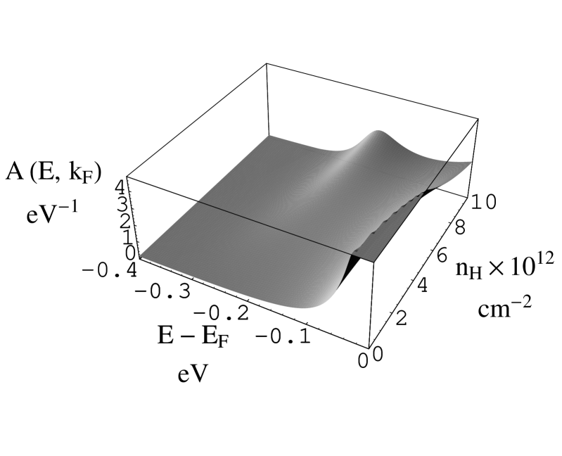
Figure 5: Evolution of the energy distribution curve at $k_{F}$ with increasing the hydrogen coverage.

It is clearly seen from the Figure that the energy width of the quasiparticle peak at $k_{F}$ is gradually increasing with increasing the hydrogen coverage. Close to the critical impurity concentration for the MIT, the width of the energy distribution curve occupies nearly all conduction band below the Fermi level, which indicates the presence of a developed quasigap in the spectrum. This broadening translates into the complete breakdown of the quasiparticle picture near the MIT. The characteristic curve shape consisting of two competing peaks reproduces well the experimentally observable one, which can be seen in Fig. 2(c) of Ref. roten, . At that, the peak, which is developing with increasing the hydrogen coverage, is connected with the impurity resonance.

Finally, we render the density plots of the spectral function (19) at hydrogen coverages that are close to the critical one for the MIT in order to reproduce Fig. 1(d) of Ref. roten, . In Fig. 6 the Fermi level is about to enter the spectral region near the resonance energy, where the quasigap is forming due to strong impurity scattering. In Fig. 7 the Fermi level is already inside the developed quasigap. The pattern of Fig. 7 suggests the apparent upturn of the dispersion as approaching the Fermi level of the system, which has been noticed in the experiment. It is worth mentioning here that point defects does not cause a uniform broadening of the spectral function, on the contrary, the impurity-induced broadening is most pronounced in the vicinity of the resonance energy $E_{r}$ in this case.

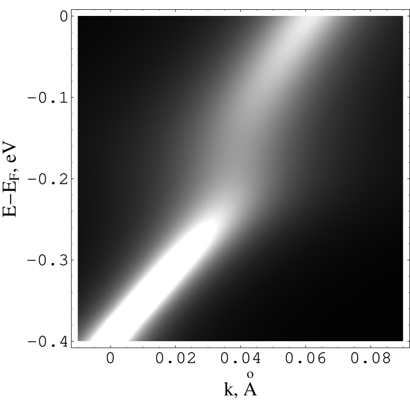
Figure 6: Density plot of the spectral function at $n_{H}=5\times 10^{12}$ cm^-2.

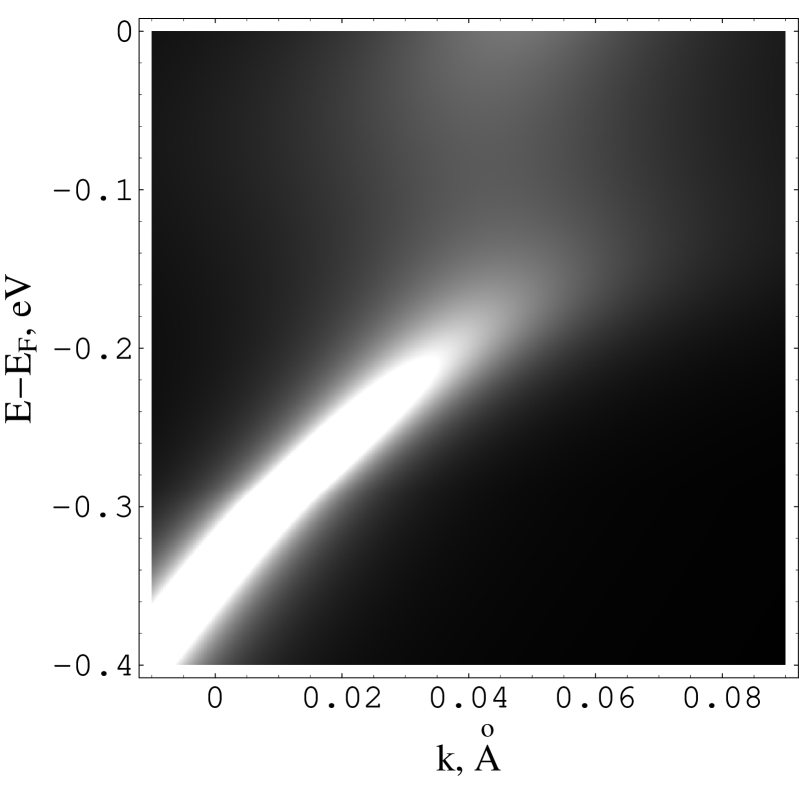
Figure 7: Density plot of the spectral function at $n_{H}=10\times 10^{12}$ cm^-2.

V Conclusion

To summarize, we have established that point defects are introducing a new length parameter into the impure graphene. This length parameter results from the presence of a single-impurity resonance and shows up as the effective radius of a single-impurity state. When the average distance between impurities decreases up to this effective radius, the quasiparticle spectrum undergoes the cardinal rearrangement. The spectrum rearrangement is manifested in the opening of the quasigap around the impurity resonance energy in the spectrum. The quasigap progressively widens with increasing the impurity concentration. The Fermi level moves due to the doping effect of impurities, as well as confining the quasigap mobility edges are moving due to its expansion. If the Fermi level crosses one of the mobility edges and enters the quasigap, where states are localized, the MIT of the Anderson type takes place in the disordered system.

We have presented arguments, which confirm that the above scenario can be considered as a sounding candidate for the explanation of the experimentally observed MIT in graphen dosed with hydrogen. Even employing the simple Lifshitz model for the impurity centers, it appears possible to achieve a semi-quantitative interpretation of the experimental data. The MIT of the Anderson type in this case is prompted by the gradual lowering of the Fermi level due to the acceptor effect of the hydrogen atoms combined with the persistent raising of the mobility edge due to the ongoing spectrum rearrangement. Thus, the spectrum rearrangement acts as the main cause of the MIT, and, as a common phenomenon in semiconductors, provides the basis for understanding the physics of the process. Indeed, the oversimplified impurity model is not able to convey all the detail of the system’s behavior. To fulfill this task, more sophisticated impurity models are required. Among them the two-parametric s-d model looks like a more natural choice for the deposited hydrogen atom. However, more sophisticated impurity models should not change the general physics of the transition process, which is already captured by the Lifshitz impurity model.

- (1) A. H. Castro Neto, F. Guinea, N. M. R. Peres, K. S. Novoselov, and A. K. Geim, Rev. Mod. Phys. 81, 109 (2009).
- (2) J. H. Bardarson, J. Tworzydlo, P. W. Brouwer, and C. W. J. Beenakker, Phys. Rev. Lett. 99, 106801 (2007).
- (3) K. Kechedzhi, E. McCann, V. I. Fal’ko, H. Suzuura, T. Ando, and B. L. Altshuler, Eur. Phys. J. Special Topics, 148, 39 (2007).
- (4) F. V. Tikhonenko, A. A. Kozikov, A. K. Savchenko, and R. V. Gorbachev, Phys. Rev. Lett. 103, 226801 (2009).
- (5) J. Bang, and K. J. Chang, Phys. Rev. 81, 193412 (2010).
- (6) J. H. Bardarson, M. V. Medvedyeva, J. Tworzydlo, A. R. Akhmerov, and C. W. J. Beenakker, Phys. Rev. B 81, 121414 (2010).
- (7) K. S. Novoselov, A. K. Geim, S. V. Morozov, D. Jiang, M. I. Katsnelson, I. V. Grigorieva, S. V. Dubonos, and A. A. Firsov, Nature 438, 197 (2005).
- (8) I. L. Aleiner, and K. B. Efetov, Phys. Rev. Lett. 97, 236801 (2006).
- (9) P. M. Ostrovsky, I. V. Gornyi, A. D. Mirlin, Phys. Rev. Lett. 98, 256801 (2007).
- (10) G. G. Naumis, Phys. Rev. B 76, 153403 (2007).
- (11) M. Amini, S. A. Jafari, and F. Shahbazi, Europhysics Lett. 87, 37002 (2009).
- (12) A. Lherbier, B. Biel, Y.-M. Niquet, and S. Roche, Phys. Rev. Lett. 100, 036803 (2008).
- (13) Y. Song, H. Song, and S. Feng, arXiv:1007.3309 (unpublished).
- (14) J.-H. Chen, C. Jang, S. Adam, M. S. Fuhrer, E. D. Williams, and M. Ishigami, Nature Phys. 4, 377 (2008).
- (15) E. R. Mucciolo, and C. H. Lewenkopf, J. Phys.: Condens. Matter 22, 273201 (2010).
- (16) N. M. R. Peres, Rev. Mod. Phys. 82, 2673 (2010).
- (17) S. Das Sarma, S. Adam, E. H. Hwang, and E. Rossi, arXiv:1003.4731 (unpublished).
- (18) V. Ugarte, V. Aji, and C. M. Varma, arXiv:1007.3533 (unpublished).
- (19) A. Bostwick, J. L. McChesney, K. V. Emtsev, T. Seyller, K. Horn, S. D. Kevan, and E. Rotenberg, Phys. Rev. Lett. 103, 056404 (2009).
- (20) F. Withers, M. Dubois, and A. K. Savchenko, Phys. Rev. B 82, 073403 (2010).
- (21) J.-H. Chen, W. G. Cullen, C. Jang, M. S. Fuhrer, and E. D. Williams, Phys. Rev. Lett. 102, 236805 (2009).
- (22) Z. H. Ni1, L. A. Ponomarenko, R. R. Nair, R. Yang, S. Anissimova, I. V. Grigorieva, F. Schedin, Z. X. Shen, E. H. Hill, K. S. Novoselov, and A. K. Geim, Nano Lett., Article ASAP (2010).
- (23) M. A. Ivanov, V. M. Loktev, and Yu. G. Pogorelov, Phys. Rep. 153, 209 (1987).
- (24) I. M. Lifshits, S. A. Gredeskul, and L. A. Pastur, Introduction to the Theory of Disordered Systems, Wiley, N.Y. (1988).
- (25) Yu. V. Skrypnyk, and V. M. Loktev, Phys. Rev. B 73, 241402(R) (2006).
- (26) S. S. Pershoguba, Yu. V. Skrypnyk, and V. M. Loktev, Phys. Rev. B 80, 214201 (2009).
- (27) A. F. Ioffe, and A. R. Regel, Prog. Semicond. 4, 237 (1960).
- (28) H. Kumazaki, and D. S. Hirashima, J. Phys. Soc. Jpn. 75, 053707 (2006).