Approximation properties of the $q$-sine bases

Abstract.

For $q\geq\frac{12}{11}$ the eigenfunctions of the non-linear eigenvalue problem associated to the one-dimensional $q$-Laplacian are known to form a Riesz basis of $L^{2}(0,1)$. We examine in this paper the approximation properties of this family of functions and its dual, and establish a non-orthogonal spectral method for the $p$-Poisson boundary value problem and its corresponding parabolic time evolution initial value problem with stochastic forcing. The principal objective of our analysis is the determination of optimal values of $q$ for which the best approximation is achieved for a given $p$ problem.

1. Introduction

The $p$-Laplace operator or $p$-Laplacian, a generalization of the ordinary Laplace operator, arises naturally in applications from physics and engineering including: slow-fast diffusion related to particles [2], superconductivity [6], wavelet inpainting [23], image processing [17] and game theory [22]. A typical application in the large $p$ limit is a model for slow-fast diffusion for sandpiles [14]. Recently there has been a significant amount of research activity encompassing methods of approximation for solution of non-linear partial differential equations involving this operator [6, 4, 3]. The aim of the present paper is to further contribute to this activity by considering the particular case of the one-dimensional $p$-Laplacian and examine in detail the approximation properties of a generalized spectral method described as follows.

Let $p>1$. For $z\in\mathbb{R}$ let $\llbracket z\rrbracket^{p-1}=z|z|^{p-2}$. By extension from the linear case corresponding to $p=2$, we define the one-dimensional $p$-Laplacian to be the differential operator $\Delta_{p}u=(\llbracket u^{\prime}\rrbracket^{p-1})^{\prime}$. Here $u:[0,1]\longrightarrow\mathbb{R}$ is such that $\llbracket u^{\prime}\rrbracket^{p-1}\in H^{1}(0,1)$. The corresponding $p$-Poisson boundary value problem is given by

(1) $$\Delta_{p}u(x)=g(x) 0\leq x\leq 1$$

$$u(0)=u(1)=0$$

where $g\in L^{2}(0,1)$. We also consider the related evolution equation

(2) $$\frac{\partial u(x,t)}{\partial t}=[\Delta_{p}u(x,t)-g(x)]+\nu\frac{\partial W(x,t)}{\partial t}$$

$$u(x,0)=0 0\leq x\leq 1$$

$$u(0,t)=u(1,t)=0 t>0$$

that includes a stochastic forcing term where the noise intensity $\nu\geq 0$ and $W$ is a space-time Wiener process. Here

(3) $$W(x,t)=\sum_{n\in\mathbb{N}}\beta_{n}(t)\psi_{n}(x)$$

where $\beta_{n}$ are independent scalar Brownian motions, $\psi_{n}$ are the eigenfunctions of the covariance operator $Q$ and $\alpha_{n}$ the corresponding eigenvalues, see [10, 21, 19]. For the case of space-time white noise we have $Q=I$. In the case of a deterministic system when $\nu=0$, (1) is the steady state solution of (2).

Let $q>1$. The so called $q$-sine functions are defined as the eigenfunctions of the $q$-Laplacian eigenvalue equation [13, 18, 20]:

(4) $$- \Delta_{q}u(x)=(q-1)\lambda\llbracket u(x)\rrbracket^{q-1} 0\leq x\leq 1$$

$$u(0)=u(1)=0.$$

This family of functions and the corresponding problem (4) was studied over 30 years ago by Elbert [13] and later by Ôtani [20], Bennewitz and Saitō [7] in connexion with the computation of optimal constants in Sobolev-type inequalities. They generalize in a natural fashion the 2-sine basis (corresponding to the linear case), and they have very similar periodicity and interlacing structures.

In [8] analogues of the classical completeness and expansion theorems for the $q$-sine functions were established for $q\geq 12/11$. Specifically it was shown that they form a Riesz basis of $L^{2}(0,1)$. This leads to the following question: what are the approximation properties of this basis, as well as its dual basis, and how they relate to the approximation properties of the standard 2-sine basis?

Below we address this question by examining approximation of the solutions of (1) and (2) via projection methods with a $q$-sine and a dual $q$-sine basis, regarding $q>1$ and $p>1$ as free parameters. A main focus of attention is the determination of optimal values of $q$ for which the highest order of convergence is achieved in a given $p$-problem. We demonstrate that standard properties of the $2$-sine basis applied to the $p=2$ problem (such as super-polynomial convergence when $g(x)$ is smooth) are lost, when a $q$-sine basis for $q\not=2$ is considered for a $p\not=2$ problem. As it turns out, the property of being a basis for the $q$-sine functions conceals a remarkably rich structure which is far from evident given the apparent simplicity of problem (4).

Background material on the $p$-sine basis and its dual is considered in §2. There we examine a matrix representation of the Schauder transform introduced in [8]. This will be crucial in our subsequent analysis as it gives rise to a stable procedure for constructing numerically both bases.

In §3 we find estimates for the approximation of square integrable functions in terms of their regularity. The dual $q$-sine basis turns out to have very similar approximation properties as the $q=2$ basis (lemma 2). On the other hand, however, it is fairly simple to construct smooth functions such that their $q$-sine Fourier coefficients do not decay faster than a power $-5/2$ for $q>2$ (lemma 3). The latter is in stark contrast with the most elementary results in the numerical approximation of solutions of differential equations by orthogonal spectral methods.

Section 4 is devoted to the $p$-Poisson boundary value problem. In theorem 5 we find explicit uniform bounds on the distance between any two solutions of (1), given the distance between the corresponding right hand sides. We then examine in detail the numerical computation of solutions of (1) for source terms that are subject to various different regularity constraints. As it turns out, the estimates established in Theorem 5 appear to be sub-optimal. A more thorough investigation in this respect will be reported elsewhere. See [11] for related results in the context of finite element approximation of the solutions of (1), including the higher dimensional case.

In the final §5 we study the numerical approximation of solutions to (2) both in the deterministic and stochastic systems. We describe our discretization strategy and solve this problem for different values of $p$ and $\nu$. Our results provide evidence on the performance of the $q$-sine basis for the solution of (2), by showing the dependence on the parameter $q$ of numerically computed $L^{2}$ residuals.

2. The $q$-sine basis and its dual

The $q$-Laplacian eigenvalue problem (4), although non-linear, has a fairly simple structure. The eigenvalues are found to be $\lambda=(n\pi_{q})^{q}$ where $\pi_{q}=\frac{2\pi}{q\sin(\pi/q)}$. The first eigenfunction $f_{1}(x)$ associated to the first eigenvalue $(\pi_{q})^{q}$ is strictly increasing in $[0,1/2]$, decreasing in $[1/2,1]$ and it is even with respect to $x=1/2$. It can be extended to an odd function (with respect to $x=0$) in the interval $[-1,1]$ and then to a $2$-periodic $C^{1}$ function of $\mathbb{R}$. If $q>2$ then $f_{1}^{\prime\prime}(x)$ is singular at $x=1/2$. The eigenfunctions $f_{n}(x)$ associated to the eigenvalues $(n\pi_{q})^{q}$ satisfy $f_{n}(x)=f_{1}(nx)$ for all $n\geq 2$.

In figure 1 we have plotted the first three eigenfunctions (top) and their corresponding derivatives (bottom) for (a) $q=1.4$ and (b) $q=10$. They typify the case $q<2$ (a) and $q>2$ (b), respectively. For large $q$ the basis functions $f_{n}$ approach zig-zag functions, which are the eigenfunctions of the $\infty$-Laplace eigenvalue problem.

Below we always assume that the family $\{f_{n}\}_{n\in\mathbb{N}}$ is normalized by the condition $f^{\prime}_{n}(0)=n\pi_{q}$ and leave implicit the dependence of $f_{n}$ on $q$. In the special case $q=2$ we write $e_{n}(x)=\sqrt{2}\sin(n\pi x)$, so that $\{e_{n}\}_{n\in\mathbb{N}}$ is an orthonormal basis.

(a)                                                                 (b)

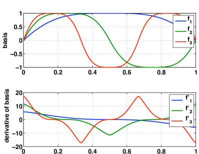
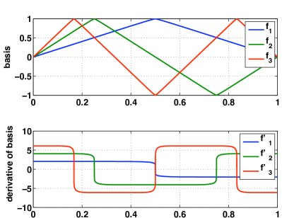
Figure 1. Approximation of the $q$-sine functions $f_{j}$ for $j=1,2,3$ (top) along with their derivatives (bottom) for (a) $q=1.4$ and (b) $q=10$.

The Pythagorean identity generalizes to the $q$-sine functions [13] as

(5) $$|f_{1}(x)|^{q}+\pi_{q}^{-q}|f_{1}^{\prime}(x)|^{q}=1.$$

Integrating this differential expression for small enough $x$ leads to the following explicit representation for the inverse function

(6) $$f_{1}^{-1}(y)=\pi_{q}^{q}\int_{0}^{y}\frac{\,\mathrm{d}x}{(1-x^{q})^{1/q}}\qquad 0\leq y\leq 1.$$

As we will see below, this representation plays a crucial role in the numerical estimation of $f_{n}(x)$.

Let the Schauder transform, $T_{q}$, be the linear extension of the mapping $e_{n}\longmapsto f_{n}$. Then $T_{q}:L^{2}(0,1)\longrightarrow L^{2}(0,1)$ is an invertible bounded operator for all $q\geq 12/11$, [8, Theorem 1]. Thus $\{f_{n}\}_{n\in\mathbb{N}}$ is a Riesz basis of $L^{2}(0,1)$ for such range of the parameter $q$. Further evidence presented in [8] suggests that in fact this is also the case for all $q>1$, but at present this has not been proved rigorously. Unless otherwise specified we will assume from now on that $q\geq 12/11$.

The property of a Riesz basis ensures that every $g\in L^{2}(0,1)$ is represented by a unique series expansion $g=\sum_{n=1}^{\infty}a_{n}f_{n}$ which is convergent in norm. The $q$-sine Fourier coefficients, $a_{n}\in\mathbb{R}$, are given explicitly by $a_{n}=\langle g,f^{*}_{n}\rangle$ where $\{f^{*}_{n}\}_{n\in\mathbb{N}}$ is the basis dual to $\{f_{n}\}_{n\in\mathbb{N}}$. Since $\delta_{jk}=\langle f_{j},f_{k}^{\ast}\rangle=\langle T_{q}e_{j},f_{k}^{\ast}\rangle=\langle e_{j},T_{q}^{\ast}f_{k}^{\ast}\rangle$ for all $j,k\in\mathbb{N}$, then $f^{\ast}_{n}=(T_{q}^{-1})^{\ast}e_{n}$. It turns out that $f_{n}^{*}\not=f_{n}$ for $q\not=2$.

The following matrix representation of $T_{q}$ is fundamental to our analysis. Let

$$\tau_{q}(j)=\widehat{f_{1}}(j)=\sqrt{2}\int_{0}^{1}f_{1}(x)\sin(j\pi x)\,\mathrm{d}x$$

be the $j$th $2$-sine Fourier coefficient of $f_{1}(x)$. Then the $k$th $2$-sine Fourier coefficient of $f_{n}(x)$ is given by

(7) $$\widehat{f_{n}}(k) =\sqrt{2}\int_{0}^{1}f_{1}(nx)\sin(k\pi x)\,\mathrm{d}x$$

$$=2\sum_{m\text{ odd}}\widehat{f_{1}}(m)\int_{0}^{1}\sin(m\pi nx)\sin(k\pi x)\,\mathrm{d}x$$

$$=\left\{\begin{array}[]{ll}\tau_{q}(m)&\text{if }mn=k\text{ for some }m\text{ odd}\\ 0&\text{otherwise.}\end{array}\right.$$

Hence $T_{q}e_{n}=\sum_{m=1}^{\infty}\tau_{q}(m)e_{mn}$ and therefore $T_{q}$ has a lower triangular matrix representation in the orthonormal basis $\{e_{n}\}_{n\in\mathbb{N}}$. See figure 2-(a).

(a)                                                                 (b)

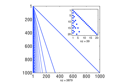
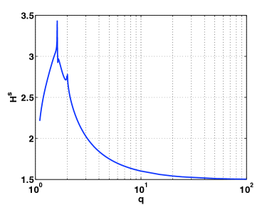
Figure 2. In (a) we plot the distribution of the non-zero entries of a $1000\times 1000$ truncation of $T_{q}$. The insert corresponds to a $20\times 20$ truncation. The matrix entries are constant along each of the “quasi-diagonals” seen in the picture. In (b) we plot $s$ against $q$ where $s$ is the numerically estimated $H^{s}$ regularity of the basis function $f_{1}(x)$. Note that at $q=2$ the regularity is infinite.

Remark 1.

The basis of eigenvectors of the $\infty$-Laplace eigenvalue problem are zig-zag functions, [8, Section 5]. In this case we can write $\tau_{\infty}(j)$ explicitly. As it turns out,

$$\lim_{q\to\infty}\tau_{q}(j)=(-1)^{j}\frac{8}{j^{2}\pi^{2}}=\tau_{\infty}(j).$$

Let $s>0$. Below we denote by $H^{s}_{\mathrm{per}}[0,1]$ the Sobolev space of 1-periodic functions $g\in L^{2}(0,1)$ such that $\sum_{j=1}^{\infty}(1+j^{2})^{s}|\widehat{g}(j)|^{2}<\infty$.

Lemma 1.

Let $f_{1}$ be the first $q$-sine function as defined above. If $1<q<2$, then $f_{1}\in H^{2}_{\mathrm{per}}[0,1]$. If $q>2$, then $f_{1}\in\bigcup_{s<3/2}H^{s}_{\mathrm{per}}[0,1]\setminus H^{3}_{\mathrm{per}}[0,1]$. If $q>4$, then $f_{1}\not\in H^{2}_{\mathrm{per}}[0,1]$.

Proof.

A straightforward argument involving integration by parts yields

$$\tau_{q}(j)=-\frac{2\sqrt{2}}{j^{2}\pi^{2}}\int_{0}^{1/2}f_{1}^{\prime\prime}(x)\sin(j\pi x)\,\mathrm{d}x.$$

Then

(8) $$|\tau_{q}(j)| \leq\frac{2\sqrt{2}}{j^{2}\pi^{2}}\int_{0}^{1/2}|f_{1}^{\prime\prime}(x)|\,\mathrm{d}x=-\frac{2\sqrt{2}}{j^{2}\pi^{2}}\int_{0}^{1/2}f_{1}^{\prime\prime}(x)\,\mathrm{d}x$$

$$=-\frac{2\sqrt{2}}{j^{2}\pi^{2}}\left[f_{1}^{\prime}(x)\right]_{0}^{1/2}=\frac{2\sqrt{2}\pi_{q}}{j^{2}\pi^{2}}.$$

Hence $\tau_{q}(j)=o(j^{-2})$ as $j\to\infty$ and $f_{1}\in\bigcup_{s<3/2}H^{s}_{\mathrm{per}}[0,1]$. From (5) it follows that $f^{\prime\prime}_{1}(x)=h(f_{1}(x))$ for $h(y)=-\pi_{q}^{2}y^{q-1}(1-y^{q})^{\frac{2-q}{q}}$.

Let $1<q<2$. Then

$$\int_{0}^{1/2}|f_{1}^{\prime\prime}(x)|^{2}\,\mathrm{d}x\leq\frac{1}{2}\max_{y\in[0,1]}|h(y)|^{2}=\frac{\pi_{q}^{4}}{2},$$

so $f_{1}\in H^{2}_{\mathrm{per}}[0,1]$.

Let $q>2$. Since $\lim_{x\to\frac{1}{2}^{\pm}}f_{1}^{\prime\prime}(x)=\mp\infty$, then $f_{1}\not\in H^{3}_{\mathrm{per}}[0,1]$. Moreover, $f_{1}(x)\geq 2x$ for $0\leq x\leq\frac{1}{2}$. Then

$$\int_{0}^{1/2}|f_{1}^{\prime\prime}(x)|^{2}\,\mathrm{d}x \geq\int_{0}^{1/2}(2x)^{2(q-1)}(1-(2x)^{q})^{\frac{2(2-q)}{q}}\,\mathrm{d}x.$$

If $q>4$, the integral on the right hand side diverges and so $f_{1}\not\in H^{2}_{\mathrm{per}}[0,1]$. ∎

Evidently the $H^{s}$ regularity for $f_{1}(x)$ found in lemma 1 is not optimal. Figure 2-(b) shows a numerical estimation of the precise value of $s(q)$, such that $f_{1}\in H^{r}_{\mathrm{per}}[0,1]$ for $r<s(q)$ and $f_{1}\not\in H^{r}_{\mathrm{per}}[0,1]$ for $r>s(q)$. The data for this graph was obtained by computing the decay rate of $\tau_{q}(j)$ for a large truncation of $T_{q}$. A thorough investigation closely related to this lemma in the higher dimensional context can be found in [5, 12] and references therein.

In the large $q$ we have a limit of $s=3/2$ and this is confirmed by Remark 1. At $q=2$ we simply have $f_{1}=\sin(\pi x)$ and so $f_{1}$ is in $H^{s}_{\mathrm{per}}[0,1]$ for all $s$. According to lemma 1, the curve should remain below $s=3$ as $q\to 2^{+}$. For $q>3$ the graph suggests $f_{1}\not\in H^{2}_{\mathrm{per}}[0,1]$. However, if $q<3$ it suggests $s(q)>2$. As $q\to 1$ the regularity drops and the limit seems to approach $s=2$. There is an interesting “peak” of regularity around $q=1.6$ which we can not presently explain.

The 2-sine Fourier coefficients of $f^{*}_{n}(x)$ are given by the $n$-th columns of $(T_{q}^{-1})^{*}$. This operator has an upper triangular representation in the 2-sine basis. Then $f^{*}_{n}(x)$ are trigonometric polynomials of order $n$. In fact, $f^{*}_{2}(x)=\tau_{q}(1)^{-1}\sin(2\pi x)$ are parallel for all $q>1$. Unlike the $q$-sine functions, not all dual $q$-sine functions have the same periodicity structure.

We now describe a stable numerical procedure for computing these two bases. The $q$-sine functions can be approximated by first estimating $f_{1}$ using (6). Numerical integration yields $f_{1}^{-1}$ on $[0,1/2]$. Although the integral is singular at $y=1$, the value $f_{1}^{-1}(1)=1/2$ is known, so we do not need to consider quadrature points too close to this singularity. In our numerical procedure we chose a fine uniform grid and apply a cumulative Simpson’s rule. This gives an approximation $\tilde{f}_{1}$ of $f_{1}$ for $x\in[0,0.5]$ with a controlled tolerance and by symmetry we obtain $\tilde{f}_{1}$ for $x\in[0,1]$. Note that $\tilde{f}_{1}$ is given on a non-uniform grid. The Pythagorean identity (5) immediate yields the derivative $f^{\prime}_{1}$ of $f_{1}$ and hence we can use it to approximate the former with a $\widetilde{f_{1}^{\prime}}$, defined also on the non-uniform grid.

Once we have constructed $\tilde{f}_{1}$ and $\widetilde{f_{1}^{\prime}}$, we use periodicity and symmetry to find corresponding approximations of $f_{n}$ and $f^{\prime}_{n}$ for $n>1$. This involves considering scaled copies $\tilde{f}_{1}$ and $\widetilde{f_{1}^{\prime}}$, to form $\tilde{f}_{n}$ and $\widetilde{f_{n}^{\prime}}$. Here the number of non-uniform grid points on $[0,1]$ grows with each $n=2:N$.

To obtain $f_{n}$ and $f_{n}^{\prime}$ on a uniform grid $x_{j}=jh$ for $j=0:J$, rather than the non-uniform grid that arises from the numerical integration, we have considered numerical interpolation by piecewise cubic polynomials. This gives $\{f^{h}_{n}\}_{n=1}^{N}$ and $\{(f^{\prime}_{n})^{h}\}_{n=1}^{N}$ defined at $x=x_{j}$. The former is the approximated basis and the latter the corresponding derivatives that we use for further computation.

Figure 1 was generated with an implementation of the numerical scheme just described on an uniform grid with $J=4000$ points ($h=2.5\times 10^{-4}$). The integral (6) was approximated with $2\times 10^{5}$ points.

The dual basis is found from an $N\times N$ truncation, $T_{q}^{N}$, of the Schauder transform. In practice, we first compute $\tau_{q}(j)$ and assemble $T^{N}_{q}$. Then we define approximations $(f^{*}_{n})^{h}$ for $n=1:N$, as the trigonometric polynomials whose $k$th 2-sine Fourier coefficients are the $(n,k)$ entry of the matrix $(T_{q}^{N})^{-1}$.

Remark 2.

In our numerical approximation of the set of basis functions we are careful to fully resolve oscillations on the basis function $f_{N}$, taking at least $20$ mesh points per wavelength and for most computations $100$ per wavelength. For $N\leq 50$ we use $h=(100N)^{-1}$ and so resolve each oscillation in the basis function with $100$ spatial points. For $N>50$ we use $h=(20N)^{-1}$ and so resolve with $20$ points. We also examined convergence of orthogonality of the basis and dual in the spatial discretization and noted $O(h^{2})$ for $q\approx 10$ through to $O(h^{4})$ for $q\approx 1.4$.

3. Approximation of source terms

Any given $g\in L^{2}(0,1)$ can be approximated by either

$$g(x)\approx g^{*}_{N}(x)=\sum_{j=1}^{N}\langle g,f_{j}\rangle f_{j}^{*}(x)\qquad\text{ or}\qquad g(x)\approx g_{N}(x)=\sum_{j=1}^{N}\langle g,f_{j}^{*}\rangle f_{j}(x)$$

for large $N$. These two expansions converge as $N\to\infty$ in the norm of $L^{2}(0,1)$ and also pointwise for almost all $x\in[0,1]$. Unlike in the linear case corresponding to $q=2$, the rates of decrease of $\|g-g^{*}_{N}\|$ and $\|g-g_{N}\|$ can be very different when $q\not=2$.

Since the dual basis $\{f^{*}_{n}\}_{n\in\mathbb{N}}$ comprises trigonometric polynomials, on the one hand we can formulate the following natural statement.

Lemma 2.

Let $g\in L^{2}(0,1)$. For all $N\in\mathbb{N}$,

$$\|g-g^{*}_{N}\|\leq\frac{\|T_{q}^{-1}\|\pi_{q}}{2\sqrt{2}}\Big{\|}g-\sum_{n=1}^{N}\widehat{g}(n)e_{n}\Big{\|}.$$

Proof.

By definition $g-g^{*}_{N}=\sum_{n=N+1}^{\infty}\langle T_{q}^{*}g,e_{n}\rangle(T_{q}^{*})^{-1}e_{n}.$ Since the matrix associated to $T_{q}^{*}$ is upper triangular (see Section 2),

$$\langle T_{q}^{*}g,e_{n}\rangle=\sum_{k=n}^{\infty}[T_{q}^{*}]_{nk}\widehat{g}(k)=\sum_{k=1}^{\infty}\tau_{q}(k)\widehat{g}(nk).$$

According to (8), we have $\sum_{k=1}^{\infty}|\tau_{q}(k)|\leq\frac{\pi_{q}}{2\sqrt{2}}$. Hence

$$|\langle T_{q}^{*}g,e_{n}\rangle|^{2} =\Big{|}\sum_{k=1}^{\infty}\tau_{q}(k)\widehat{g}(nk)\Big{|}^{2}=\Big{|}\sum_{k=1}^{\infty}\tau_{q}(k)^{1/2}\tau_{q}(k)^{1/2}\widehat{g}(nk)\Big{|}^{2}$$

$$\leq\Big{(}\sum_{k=1}^{\infty}|\tau_{q}(k)|\Big{)}\Big{(}\sum_{k=1}^{\infty}|\tau_{q}(k)||\widehat{g}(nk)|^{2}\Big{)}\leq\frac{\pi_{q}}{2\sqrt{2}}\sum_{k=1}^{\infty}|\tau_{q}(k)||\widehat{g}(nk)|^{2}.$$

Thus,

$$\|g-g_{N}^{*}\|^{2} \leq\|T_{q}^{-1}\|^{2}\sum_{n=N+1}^{\infty}|\langle T_{q}^{*}g,e_{n}\rangle|^{2}\leq\|T_{q}^{-1}\|^{2}\frac{\pi_{q}}{2\sqrt{2}}\sum_{n=N+1}^{\infty}\sum_{k=1}^{\infty}|\tau_{q}(k)||\widehat{g}(nk)|^{2}$$

$$=\|T_{q}^{-1}\|^{2}\frac{\pi_{q}}{2\sqrt{2}}\sum_{k=1}^{\infty}\sum_{n=N+1}^{\infty}|\tau_{q}(k)||\widehat{g}(nk)|^{2}=\|T_{q}^{-1}\|^{2}\frac{\pi_{q}}{2\sqrt{2}}\sum_{k=1}^{\infty}|\tau_{q}(k)|\sum_{n=N+1}^{\infty}|\widehat{g}(nk)|^{2}$$

$$\leq\|T_{q}^{-1}\|^{2}\frac{\pi_{q}}{2\sqrt{2}}\sum_{k=1}^{\infty}|\tau_{q}(k)|\sum_{n=N+1}^{\infty}|\widehat{g}(n)|^{2}=\|T_{q}^{-1}\|^{2}\frac{\pi_{q}^{2}}{8}\sum_{n=N+1}^{\infty}|\widehat{g}(n)|^{2}.$$

∎

Therefore the $q$-sine dual expansion of any $g\in C^{\infty}$ converges super-polynomially fast. On the other hand, however, it is not difficult to construct examples of smooth functions $g$ with a subsequence of $q$-sine Fourier coefficients decaying slowly.

Lemma 3.

Let $g(x)=e_{1}(x)$. If $j$ is prime, then $\langle g,f_{j}^{*}\rangle=\tau_{q}(j)\tau_{q}(1)^{-1}.$

Proof.

Since $T_{q}$ has an (infinite) lower triangular matrix representation in the orthonormal basis $\{e_{n}\}_{n\in\mathbb{N}}$, we can find the entries of the corresponding matrix representation of $T_{q}^{-1}$ by pivoting and forward substitution (Gaussian elimination). It is readily seen that $T_{q}^{-1}$ is necessarily lower triangular and its diagonal should be constant and equal to $\tau_{q}(1)^{-1}$.

Assume that $j$ is prime. According to (7), the only non-zero entries in the $j$th row of $T_{q}$ are $\tau_{q}(j)$ in the first position and $\tau_{q}(1)$ in the $j$th position. Therefore, the only non-zero entries in the $j$th row of $(T_{q})^{-1}$ are $-\frac{\tau_{q}(j)}{\tau_{q}(1)}$ in the first position and $\tau_{q}(1)^{-1}$ in the $j$th position. As the Fourier sine coefficients of $f_{j}^{*}$ are obtained from the $j$th column of $(T_{q}^{*})^{-1}$, the desired conclusion follows. ∎

By virtue of lemma 1, the prime $q$-sine Fourier coefficients of $\sin(\pi x)$ for $q>2$ can not decrease faster than $j^{-5/2}$ in the large $j$ limit. Observe that this is in stark contrast with the most elementary results in the numerical approximation of solutions of differential equations by orthogonal spectral methods.

Remark 3.

The finite set of basis functions $f_{n}$ and dual $f_{n}^{*}$ for $n=1:N$ generate corresponding $N$ dimensional subspaces $V_{N}$ and $V_{N}^{*}$ of $L^{2}(0,1)$. Instead of computing directly with these non-orthogonal bases, one can apply the Gram-Schmidt algorithm in order to obtain orthonormal bases of these subspaces. This has a numerical advantage of not needing to store both the basis and dual. We also considered this approach, however we found little advantage in terms of accuracy.

Let us now consider various numerical tests on the approximation of regular functions by $\{f_{n}\}_{n\in\mathbb{N}}$ and $\{f_{n}^{*}\}_{n\in\mathbb{N}}$. Once the bases have been obtained on uniform mesh, we can examine their approximation properties numerically by looking at the decay of suitable residual for benchmark sources $g\in L^{2}(0,1)$.

Figure 3 shows the typical outcomes of an experiment to determine the dependence in $q$ of the $L^{2}(0,1)$ residual. We have fixed here $N=40$, varied $q=1:100$, and computed residuals in the approximation of the following four functions:

(9) $$\begin{gathered}g_{\mathrm{a}}(x)=f_{1}(x)+(2.5)f_{10}(x)\qquad\text{for }\quad q=10,\\ g_{\mathrm{b}}(x)=\left\{\begin{array}[]{ll}1&x\in[1/4,3/4]\\ 0&\text{otherwise}\end{array}\right.\\ g_{\mathrm{c}}(x)=\left\{\begin{array}[]{ll}(7/3)x&x\in[0,3/7]\\ -(21/4)x+13/4&x\in[3/7,7/14]\\ (21/4)x-2&x\in[7/14,4/7]\\ -x+11/7&x\in[4/7,1]\end{array}\right.\\ g_{\mathrm{d}}(x)=(q-1)(k\pi_{q})^{q}f_{1}|f_{1}|^{(q-2)}\qquad\text{for }\quad q=3,\end{gathered}$$

in (a)-(d) respectively. In the figure we include both the basis and its dual, as well analogous calculations with the orthogonalized bases of $V_{40}$ and $V_{40}^{*}$. In (a) we see an optimal ${q_{\text{opt}}}=10$ as expected, in (b), (c) and (d) we increase the regularity of $g$ and see ${q_{\text{opt}}}$ decrease with values of $4.25,\,2.9,\,2.55$ for (b), (c) and (d) respectively.

(a)                                                                 (b)

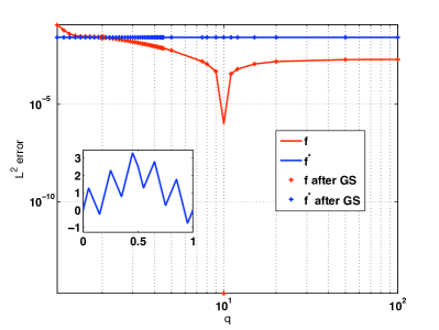
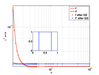
(c)                                                                 (d)

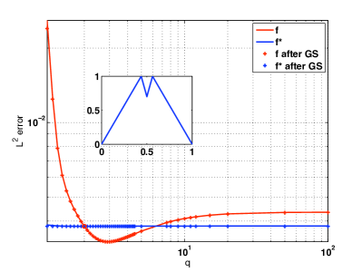
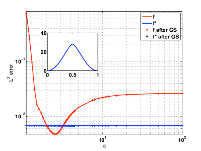
Figure 3. We vary a $q$-sine basis and dual basis and examine how the residual changes using $N=40$ modes for (a) $g$ a combination of two $10$-sine basis elements, (b) a piece-wise constant function ${q_{\text{opt}}}\approx 4.25$, (c) a piece-wise linear continuous ${q_{\text{opt}}}=2.9$ and (d) a differentiable with discontinuous derivative function ${q_{\text{opt}}}=2.55$. See (9).

This experiment gives a general insight about the $q$-behavior of $L^{2}$-residuals in the approximation of functions with different degrees of regularity by $q$-sine bases and their duals. For the simple functions considered, our calculations indicate the following general behavior of the $q$-sine basis:

• as $q\to 1$ the residual deteriorates,

• there is always a single minimum corresponding to an optimal $q=q_{\mathrm{opt}}$,

• as $q\to\infty$ the residual curve becomes asymptotically constant with no local maximum for $q>2$.

In contrast, the approximation error is almost constant in $q$ for the $q$-sine dual basis. This is indeed a consequence of Lemma 2 and the fact that $f_{n}^{*}$ are trigonometric polynomials. Our tests indicate that there does not seem to be a clear advantage in orthogonalizing the basis or the dual basis for errors with an order of magnitude above $10^{-5}$.

$g(x)$	$q=1.8$	$q=2$ (exact)	$q=3$	$q=5$	$q=10$
$g_{\mathrm{b}}(x)$	-0.4862	-0.4905 (-0.5)	-0.5005	-0.5052	-0.5069
$g_{\mathrm{c}}(x)$	-1.4266	-1.4474 (-1.5)	-1.4959	-1.4842	-1.4438
$g_{\mathrm{d}}(x)$	-1.9368	-1.9952 (-2)	-1.9826	-1.5934	-1.4595
$\sin(\pi x)$	-2.2778	NaN $(-\infty)$	-1.9560	-1.6237	-1.4988

Table 1. Rates of convergence in $N$ for $g$ with different degrees of regularity and selected values of $q$.

In table 1 we have estimated $\alpha>0$ such that $\|g-g_{N}\|<\beta N^{-\alpha}$ where $\beta>0$ is independent of $N$. The data indicates that for $g\in H^{1}_{\mathrm{per}}[0,1]$, $q_{\mathrm{opt}}\approx 2$. Moreover, as $q$ increases, we should expect $\alpha$ to decrease and stabilize always below $1.5$ for $g(x)=\sin(\pi x)$. This is indeed suggested by lemma 1, figure 2-(b) and lemma 3, and it is confirmed by the last row of the table.

(a)                                            (b)                                            (c)

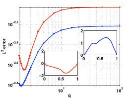
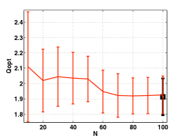
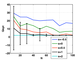
Figure 4. In (a) $L^{2}$ residual as a function of $q$ where a $q$-sine basis is used to approximate two different randomly generated $g\in H^{2}_{\mathrm{per}}[0,1]$ satisfying $g(0)=g(1)=0$. Note that the optimal ${q_{\text{opt}}}$ occurs at different values. In (b) and (c) we examine ${q_{\text{opt}}}$ as $N$ increases. We include the mean and standard deviation over $200$ realizations of random functions subject to the same constraint. For $N=100$ we also show the results from $1000$ realizations.

In figure 4-(a) we have computed the residual $\|g-g_{10}\|$ (red) and $\|g-g_{20}\|$ (blue) for randomly generated $g\in H^{2}_{\mathrm{per}}[0,1]$ constrained to $g(0)=g(1)=0$. To construct a random function $g$ such that the $H^{s}_{\mathrm{per}}[0,1]$ norm is finite, we find $\widehat{g}(j)=a_{j}\beta_{j}$ where $a_{j}=(1+j^{2})^{-s/2}|j|^{-\frac{1}{2}-\delta}$ for some small $\delta>0$ and $\beta_{j}$ are independent identically distributed $N(0,1)$. Two realizations of functions $g$ obtained in this way are shown in the inserts in figure 4. Note that ${q_{\text{opt}}}$ is achieved at different places but close to $2$. In figure 4-(b) we examine ${q_{\text{opt}}}$ over $200$ realizations of functions in $H^{2}_{\mathrm{per}}[0,1]$. For any fixed realization and value of $N$, ${q_{\text{opt}}}\neq 2$ although in the limit this optimal parameter appears to be close to 2. For $N=100$ we also show the results of $1000$ realizations. In this case, the mean value is closer to $2$ although the variation is still large. In figure 4-(c) we show the mean values where functions are taken in $H^{s}_{\mathrm{per}}[0,1]$ for $s=-0.5,\,0,\,0.5,\,1$ and $2$ with $200$ realizations. For $s<2$ the variability in ${q_{\text{opt}}}$ is far larger. For fixed $N$, ${q_{\text{opt}}}>2$.

The observed outcome of this experiment strongly support the conjecture that $q_{\mathrm{opt}}$ typically approaches $2$ as the regularity of $g$ is increased.

4. Numerical solution of the $p$-Poisson equation

We now address the question of approximating the solutions of (1) by means of a $q$-sine and dual basis. In view of lemmas 2 and 3, we begin by determining uniform estimates on how sensitive this solution is under perturbations of the right hand side. Analogous questions have certainly been considered in more general frameworks, however here we focus on the explicit calculation of the constants involved.

A key ingredient in the estimates presented below is the fact that (1) can be integrated explicitly. Let the Volterra operator

$$Vg(x)=\int_{0}^{x}g(t)\,\mathrm{d}t.$$

Note that $Vg\in H^{1}(0,1)$ for all $g\in L^{1}(0,1)$. Furthermore $V:L^{s}(0,1)\longrightarrow L^{t}(0,1)$ is a contraction operator for all $1\leq s,t\leq\infty$ and its norm can be explicitly determined [7, Theorem 1.1]. Let

$$h_{g}(\gamma)=\int_{0}^{1}\llbracket Vg(\tau)-\gamma\rrbracket^{\frac{1}{p-1}}\,\mathrm{d}\tau.$$

Then $h_{g}(\gamma)$ is a continuous function, decreasing in $\gamma$, for all fixed $g\in L^{1}(0,1)$. Let

$$\min_{x\in[0,1]}Vg(x)\leq\gamma_{0}(g)\leq\max_{x\in[0,1]}Vg(x)$$

be the unique root such that $h_{g}(\gamma_{0}(g))=0$. Then

(10) $$u(x)=\int_{0}^{x}\llbracket Vg(\tau)-\gamma_{0}(g)\rrbracket^{\frac{1}{p-1}}\,\mathrm{d}\tau=V\left(\llbracket Vg(\tau)-\gamma_{0}(g)\rrbracket^{\frac{1}{p-1}}\right)(x)$$

is the unique solution of (1).

We firstly establish concrete Hölder estimates on $h_{g}(\gamma)$. Without further mention in this section we will fix $r=\frac{1}{p-1}$ and denote by $\|\!\cdot\!\|_{s}$ the norm of $L^{s}(0,1)$. In the case $s=2$ we will continue suppressing the sub-index.

Lemma 4.

Let $g\in L^{1}(0,1)$ and $-\|g\|_{1}\leq\gamma\leq\mu\leq\|g\|_{1}$. Then

$$(\mu-\gamma) \leq\frac{2^{1-r}\|g\|_{1}^{1-r}}{r}[h_{g}(\gamma)-h_{g}(\mu)] 0<r\leq 1$$

$$(\mu-\gamma)^{r} \leq 2^{r-1}[h_{g}(\gamma)-h_{g}(\mu)] r>1.$$

Proof.

Suppose first that $0<r\leq 1$. From the graph of $\llbracket z\rrbracket^{r}$ for $|z|\leq M$ it is readily seen that $\llbracket z\rrbracket^{r}-\llbracket w\rrbracket^{r}\geq rM^{r-1}(z-w)$ for all $-M\leq w\leq z\leq M$. Then

$$(\mu-\gamma) =\int_{0}^{1}\left[(Vg(\tau)-\gamma)-(Vg(\tau)-\mu)\right]\,\mathrm{d}\tau$$

$$\leq\frac{M^{1-r}}{r}\left[h_{g}(\gamma)-h_{g}(\mu)\right]$$

for $M=2\|g\|_{1}$, and $\gamma$ and $\mu$ as in the hypothesis.

In a similar fashion, let $r>1$. Then $(z-w)^{r}\leq 2^{r-1}(\llbracket z\rrbracket^{r}-\llbracket w\rrbracket^{r})$ for all $-M\leq w\leq z\leq M$. Indeed, if $0\leq w<z$, a straightforward argument shows that

$$\frac{\llbracket z\rrbracket^{r}-\llbracket w\rrbracket^{r}}{z-w}=\frac{z^{r}-w^{r}}{z-w}\geq z^{r-1}\geq(z-w)^{r-1};$$

if $w<z\leq 0$,

$$\frac{\llbracket z\rrbracket^{r}-\llbracket w\rrbracket^{r}}{z-w}\geq|w|^{r-1}\geq(z-w)^{r-1};$$

and if $w<0<z$,

$$\min_{z>0}\frac{\llbracket z\rrbracket^{r}-\llbracket w\rrbracket^{r}}{(z-w)^{r}}=\min_{z>0}\frac{z^{r}-|w|^{r}}{(z+|w|)^{r}}=\frac{1}{2^{r-1}}$$

achieved when $w=-z$. Thus

$$(\mu-\gamma)^{r} =\int_{0}^{1}\left[(Vg(\tau)-\gamma)-(Vg(\tau)-\mu)\right]^{r}\,\mathrm{d}\tau$$

$$\leq 2^{r-1}\left[h_{g}(\gamma)-h_{g}(\mu)\right].$$

∎

Theorem 5.

Let $u$ and $\tilde{u}$ be solutions of (1) with corresponding sources $g$ and $\tilde{g}$. Let $m=\max\{\|g\|_{1},\|\tilde{g}\|_{1}\}$. Then

$$\|u-\tilde{u}\| \leq 2^{1-r}\left(\|g-\tilde{g}\|+\frac{(4m)^{1-r}}{r}\|g-\tilde{g}\|_{1}^{r}\right)^{r} 0<r\leq 1$$

$$\|u-\tilde{u}\| \leq r2^{r-1}m^{r-1}\left(\|g-\tilde{g}\|+2^{2-2/r}m^{1-1/r}r^{1/r}\|g-\tilde{g}\|_{1}^{1/r}\right) r>1.$$

Proof.

Let $0<r\leq 1$ and $s=2/r\geq 2$. By virtue of (10)

$$\|u-\tilde{u}\|\leq\big{\|}V\left(\llbracket Vg-\gamma_{0}(g)\rrbracket^{r}-\llbracket V\tilde{g}-\gamma_{0}(\tilde{g})\rrbracket^{r}\right)\big{\|}_{s}\leq\big{\|}\llbracket Vg-\gamma_{0}(g)\rrbracket^{r}-\llbracket V\tilde{g}-\gamma_{0}(\tilde{g})\rrbracket^{r}\big{\|}_{s}.$$

Note that $|\llbracket z\rrbracket^{r}-\llbracket w\rrbracket^{r}|\leq 2^{1-r}|z-w|^{r}$ for all $0\leq|w|\leq|z|$. Thus

$$\big{\|}\llbracket Vg-\gamma_{0}(g)\rrbracket^{r}-\llbracket V\tilde{g}-\gamma_{0}(\tilde{g})\rrbracket^{r}\big{\|}_{s}^{1/r} \leq 2^{\frac{1-r}{r}}\left(\|V(g-\tilde{g})\|+|\gamma_{0}(\tilde{g})-\gamma_{0}(g)|\right)$$

$$\leq 2^{\frac{1-r}{r}}\left(\|g-\tilde{g}\|+|\gamma_{0}(\tilde{g})-\gamma_{0}(g)|\right).$$

According to lemma 4,

$$|\gamma_{0}(\tilde{g})-\gamma_{0}(g)| \leq\frac{(2m)^{1-r}}{r}|h_{g}(\gamma_{0}(\tilde{g}))-h_{g}(\gamma_{0}(g))|=\frac{(2m)^{1-r}}{r}|h_{g}(\gamma_{0}(\tilde{g}))-h_{\tilde{g}}(\gamma_{0}(\tilde{g}))|$$

$$\leq\frac{(2m)^{1-r}}{r}\int_{0}^{1}\Big{|}\llbracket Vg-\gamma_{0}(\tilde{g})\rrbracket^{r}-\llbracket V\tilde{g}-\gamma_{0}(\tilde{g})\rrbracket^{r}\Big{|}\,\mathrm{d}\tau$$

$$\leq\frac{(4m)^{1-r}}{r}\|g-\tilde{g}\|_{r}^{r}\leq\frac{(4m)^{1-r}}{r}\|g-\tilde{g}\|_{1}^{r}.$$

This ensures the first statement.

Let $r>1$. In a similar fashion as before, we see that

$$\|u-\tilde{u}\| \leq\big{\|}\llbracket Vg-\gamma_{0}(g)\rrbracket^{r}-\llbracket V\tilde{g}-\gamma_{0}(\tilde{g})\rrbracket^{r}\big{\|}$$

$$\leq r2^{r-1}m^{r-1}\left(\|V(g-\tilde{g})\|+|\gamma_{0}(g)-\gamma_{0}(\tilde{g})|\right)$$

$$\leq r2^{r-1}m^{r-1}\left(\|g-\tilde{g}\|+|\gamma_{0}(g)-\gamma_{0}(\tilde{g})|\right).$$

Lemma 4 and similar arguments as for the previous case, yield

$$|\gamma_{0}(\tilde{g})-\gamma_{0}(g)|^{r} \leq 2^{r-1}\left|h_{\tilde{g}}(\gamma_{0}(\tilde{g}))-h_{g}(\gamma_{0}(\tilde{g}))\right|$$

$$\leq 2^{2r-2}m^{r-1}r\|g-\tilde{g}\|_{1}.$$

This completes the proof. ∎

The right hand side bound in the above theorem approaches 2 as $r\to 0$ independently of the value of $\|g-\tilde{g}\|$. In fact $\|u-\tilde{u}\|\leq\left\|l_{r}\right\|_{1}$ for $l_{r}=\llbracket Vg-\gamma_{0}(g)\rrbracket^{r}-\llbracket V\tilde{g}-\gamma_{0}(\tilde{g})\rrbracket^{r}$. Since $l_{r}(\tau)\to 0$ for almost all $\tau\in[0,1]$ and $|l_{r}(\tau)|\leq 2+\|Vg\|_{\infty}+\|V\tilde{g}\|_{\infty}$, the Dominated Convergence Theorem yields $\|u-\tilde{u}\|\to 0$ as $r\to 0$. This is a well-known property of the $\infty$-Laplacian, see [22]. As mentioned in the introduction, the approach considered in [11] in the context of finite element approximation of the solutions of (1), may provide an insight on whether the constants found in the above theorem are optimal.

(a)                                                                 (b)

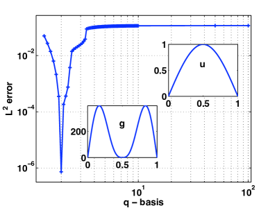
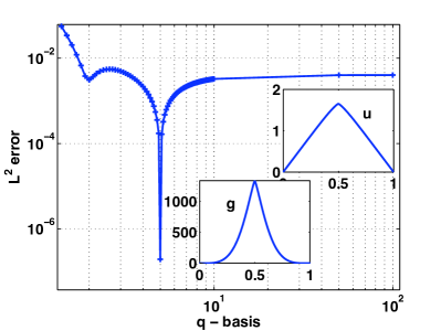
Figure 5. Solving the $p$-Laplacian problem with $p=5$. (a) The most accurate basis for a solution $u(x)=\sin(\pi x)$ is the standard 2-sine basis. (b) However for a solution $u(x)=f_{1}(x)$ with $q=5$ the 5-sine basis is the most accurate.

We now describe how the $p$-Poisson problem is discretized. The strong formulation (1) leads to the following weak formulation using integration by parts and the boundary conditions:

(11) $$\int_{0}^{1}|u^{\prime}|^{p-2}u^{\prime}v^{\prime}\,\mathrm{d}x=\int_{0}^{1}gv\,\mathrm{d}x$$

for any absolutely continuous test function $v$. We expand both $u$ and $v$ using a basis $\{\phi_{n}\}_{n\in\mathbb{N}}$, where $\phi_{n}$ is either $f_{n}$ or $f_{n}^{*}$. After truncation this leads to the following nonlinear system of equations for unknown coefficients $c_{j}=\langle u,\phi_{j}^{*}\rangle$:

(12) $$\sum_{k=1}^{N}c_{k}\int_{0}^{1}\left|\sum_{\ell=1}^{N}c_{\ell}\phi_{\ell}^{\prime}\right|^{p-2}\phi_{k}^{\prime}\phi_{j}^{\prime}\,\mathrm{d}x=\langle g,\phi_{j}\rangle\qquad j=1:N.$$

The case $p=2$ evidently reduces to the standard linear system to solve for the Poisson equation.

(a)                                                                 (b)

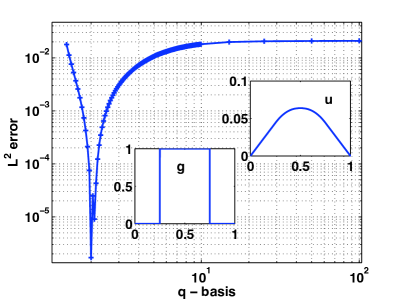
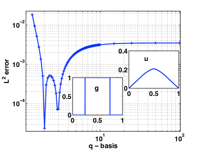
(c) (d)

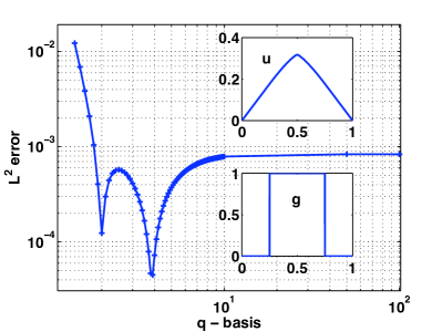
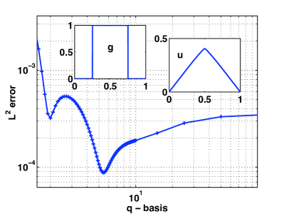
Figure 6. We now examine a piecewise constant $f$ for different $p$ ($N=40$). In (a) $p=1.8$ and ${q_{\text{opt}}}=2$ (b) $p=3$ and ${q_{\text{opt}}}\approx 2$ with another minimum at $q=2.95$, in (c) $p=5$ and ${q_{\text{opt}}}\approx 3.9$ and in (d) $p=10$ and ${q_{\text{opt}}}\approx 5.75$.

Numerically the right hand side of (12) is approximated via quadrature rules. The nonlinear system may then be solved for example by Newton’s method. Since the Jacobian is a full matrix in this case, a banded approximation appears to provide sufficient accuracy. However, the results presented below were found using the trust-region dogleg method with a full Jacobian matrix as implemented in Matlab.

(a)                                                                 (b)

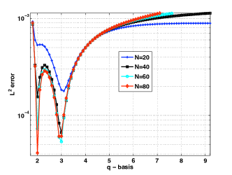
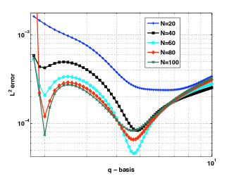
(c)                                                                 (d)

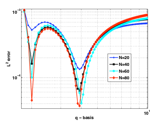
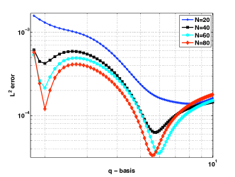
Figure 7. Comparison of $N=20,40,60,80$ in (a) for $p=5$ and $g\equiv 1$ (b) for $p=10$ and $g\equiv 1$ (also including $N=100$). In (c) we show for $g\equiv g_{\mathrm{b}}$ and $p=5$, and in (d) for $g\equiv g_{\mathrm{b}}$ and $p=10$. We note that for $N$ sufficiently large ${q_{\text{opt}}}=2$, and a more accurate solution may be found for smaller $N$ at ${q_{\text{opt}}}\neq 2$.

In figure 5 we have use this scheme to solve the $p$-Laplacian problem with $p=5$ and examine the $L^{2}$ error taking $N=40$. In figure 5-(a) we have fixed a solution $u(x)=\sin(\pi x)$ where we clearly expect and observe that $q=2$ is the optimal basis. In figure 5-(b) we have fixed $u(x)=f_{1}(x)$ for $p=5$ and so we observe the $q=5$ as the optimal basis.

g	$p=1.8$	$p=3$	$p=5$	$p=10$
$g_{\mathrm{b}}$ $(N=20)$	2.05	2.95	3.9	8.0
$g_{\mathrm{b}}$ $(N=40)$	2.05	2.0 (2.95)	3.9	5.75
$g_{\mathrm{b}}$ $(N=60)$	2.2	3.0	4.0	5.95
$g_{\mathrm{b}}$ $(N=80)$	2.05	2.0	3.9	5.60
$g=1$ $(N=20)$	2.0	2.3	3.1	6.43
$g=1$ $(N=40)$	2.0	2.0	3.0	4.85
$g=1$ $(N=60)$	2.0	2.0	3.0	4.7
$g=1$ $(N=80)$	2.0	2.0	2.0 (2.95)	4.7

Table 2. Optimal ${q_{\text{opt}}}$ for four different $p$-Laplacian problems with either a $g=g_{\mathrm{b}}$ from (9) or $g=1$. We give estimates for different values of $N$. The change in ${q_{\text{opt}}}$ as $N$ increases occurs as the two minima interchange, see figures 6 and 7.

In figure 6 we take $g=g_{\mathrm{b}}$ from (9) which turns out to be a typical form of forcing for sandpile problems. We solve the $p$-Laplacian problem for (a) $p=1.8$, (b) $p=3$, (c) $p=5$ and $p=10$ with $N=40$ and examine the $L^{2}$ error in the solution as we vary the $q$ basis. To estimate this error we take as exact the solution with 2-sines and $2N$ modes. We observe that the optimal basis for representing the solutions is no longer the standard $q=2$ for $p=3,5,10$. For problems with moderate $p$ (for example $p=3$) we see two distinct minima. For larger $p$ problems however, the $q=2$ basis becomes less competitive.

In table 2 we give estimates of ${q_{\text{opt}}}$ for $g=g_{\mathrm{b}}$ and $g=1$ for $N=20,40,60$ and $N=80$ modes. The changes in ${q_{\text{opt}}}$ with $N$ are explained by the interchange of the two minima in figure 6. For $N=100$ this interchange occurs for $p=5$ and $p=10$ as illustrated in figure 7-(b).

5. The time dependent $p$-Laplacian

In this final section we consider the evolution equation (2) both in the deterministic ($\nu=0$) and the stochastically forced regime ($\nu\neq 0$). Slow-fast diffusion is often taken in the large $p$ limit, as a model for sandpile growth. For further details including arguments about the validity of the modeling see for example [15, 2, 16, 14, 1, 9]. Our purpose here is to consider the time dependent problem for different values of $p$ and examine the choice of basis in the formation of the sandpile.

We discretize the weak form of the equation and truncate to solve the time-dependent version of (12) given by

(13) $$\frac{dc_{j}}{dt}=\sum_{k=1}^{N}c_{k}\int_{0}^{1}\left|\sum_{\ell=1}^{N}c_{\ell}\phi_{\ell}^{\prime}\right|^{p-2}\phi_{k}^{\prime}\phi_{j}^{\prime}dx-\langle g,\phi_{j}\rangle+\nu\langle\frac{dW}{dt},\phi_{j}\rangle\qquad j=1:N.$$

This expression is then discretized in time to get a nonlinear system of equations to solve for $c_{j}^{n}$ at each step. Below we consider an Euler’s method which reduces to

$$\frac{c^{n+1}_{j}-c^{n}_{j}}{{\Delta t}}=\sum_{k=1}^{N}c_{k}^{n+1} \int_{0}^{1}\left|\sum_{\ell=1}^{N}c_{\ell}^{n+1}\phi_{\ell}^{\prime}\right|^{p-2}\phi_{k}^{\prime}\phi_{j}^{\prime}dx$$

$$-\langle\phi_{j}^{*},g\rangle+\nu\langle\phi_{j}^{*},\sum_{m=1}^{M}\alpha_{j}^{1/2}e_{j}(x)\Delta\beta_{m}\rangle$$

where $\Delta\beta_{m}$ are independent identically distributed random variables with mean zero and variance ${\Delta t}$ (recall (3)), and we have assumed the eigenfunctions of $Q$ are now given by $e_{n}$. For the case of stochastic forcing we take $M>>N$.

(a)                                                                 (b)

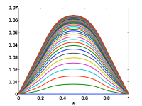
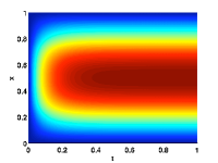
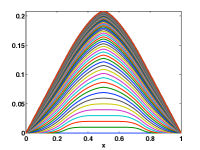
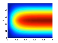
(c)                                                                 (d)

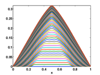
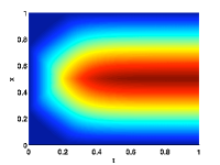
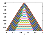
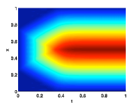
Figure 8. Solution of (2) with $g=g_{\mathrm{b}}$ for (a) $p=1.8$ using $q=2$, (b) $p=3$ using $q=2.95$, (c) $p=5$ using $q=3.9$ and (d) $p=10$ using $q=5.75$. As time evolves the solutions approach the steady state which, for increasing $p$, turns out to be close to a hat function.

In figure 8 we consider $\nu=0$ with $g=g_{\mathrm{b}}$ and we plot the time evolution for (a) $p=1.8$ (${q_{\text{opt}}}=2$), (b) $p=3$ (${q_{\text{opt}}}=2.95$), (c) $p=5$ (${q_{\text{opt}}}=3.9$) and (d) $p=10$ (${q_{\text{opt}}}=5.75$). In each case the evolution found numerically quickly converges towards the steady state.

(a)                                                      (b)

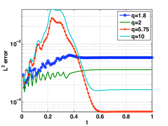
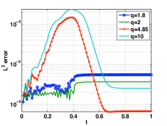
Figure 9. Residual in time for the numerical solution of (2). We choose $\nu=0$, $N=40$ and take as a true solution one computed with $N=100$ and $q=2$. We fix $p=10$ and compare basis with $q=1.8$, $q=2$, $q={q_{\text{opt}}}$ and $q=10$. Here (a) corresponds to $g=g_{\mathrm{b}}$ (${q_{\text{opt}}}=5.75$) and (b) to $g=1$ (${q_{\text{opt}}}=4.85$). We see that asymptotically in time ${q_{\text{opt}}}$ has the smallest error. At a few points in time during the transient state, the $q=1.8$ basis is more accurate than the $q=2$.

Figure 8 was obtained by choosing in each case the predicted $q={q_{\text{opt}}}$ basis for the steady state. Intuitively this choice of basis should be near optimal for large $t$. On the other hand however, there is no reason to presume that it is so for small values of $t$. In figure 9 we examine the spatial error at each step for four different bases with $N=40$. For comparison we have chosen $p=10$ and $q\in\{1.8,2,{q_{\text{opt}}},10\}$. As the solution approaches the steady state, in each case the basis ${q_{\text{opt}}}$ has the smallest error as is expected (in fact a gain of almost an order of magnitude in accuracy compared to $q=2$ is observed). It is remarkable however that, in the transient regime, these bases appear to be far less accurate than other choices of $q$, such as $q=2$ and $q=1.8$.

(a)                                            (b)                                            (c)

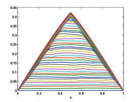
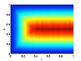
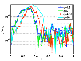
(d)                                            (e)                                            (f)

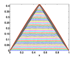
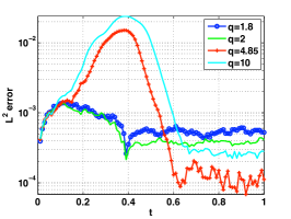
Figure 10. Sample realization with $p=10$ of the time evolution problem with a time-dependent stochastic forcing $\nu=0.2$. The time evolution is shown with equal steps of ${\Delta t}=0.01$. In (a)-(c) we show the effect of an $H^{1}$ noise in space, white in time. In (d)-(f) we show the effect of a white noise in both space and time.

Let us now consider the stochastically forced case, $\nu>0$. Figure 10 shows plotted solution with time dependent noises which are: $H^{1}$ in space and white in time for (a)-(c), and white both in space and time for (d)-(f). The forcing corresponds to $\nu=0.2$. We expect that on average the noisy solution is simply that of the deterministic system (which has a unique stable solution). We see in (a)-(b) and (d)-(e) the time evolution of the solution for one particular realization of the noise. This should be compared with the deterministic case in figure 8-(d).

In figure 10-(c) and figure 10-(f) we plot the evolution of the error for fixed time-step with $q\in\{1,2,{q_{\text{opt}}},10\}$. Similar to the deterministic case, in the transient regime the error for ${q_{\text{opt}}}$ and $q=10$ is far higher than that for $q=2$ or $q=1.8$. Where the noise effects are large (such as for the spatially correlated noise in $H^{1}$ in figure 10-(c)), the optimal basis is no longer clear. However where the effect is small (such as the white noise in figure 10-(f)), we clearly see in the time dependent evolution about the steady state that the $q=4.85$ outperforms the other bases (and in particular $q=2$). For sandpile-type problems the introduction of a spatially white noise is a natural choice. It is interesting to note the small effect on the dynamics in this realization.

At present it is unclear whether the use of a $q$-sine basis with $q\not=2$ provides any real computational advantage over the natural choice $q=2$ for the solution of (2). There is clearly a computational overhead in obtaining the former for $q\neq 2$ that impacts significantly on efficiency. However we have observed that the nonlinear problem (12) is solved faster in the optimal basis. This is certainly worth further investigation. For example for $N=40$ we observe approximately a 20% speed up in the nonlinear solve over the standard 2-sine basis. Thus, if solving many fixed $p$-problems, the corresponding optimal $q$-sine basis may not only be more accurate but also more efficient. In our current implementation the $q$-sine basis may be precomputed and stored. Lemma 1 give some prelimeinary indication on how to solve the problem of apriori determining the optimal basis. Our numerical results suggest that for large $p$ we expect an optimal basis with $q>2$ for a right hand side with a discontinuous derivative.

References

Andreu et al. [2009]
F. Andreu, J. M. Mazón, J. D. Rossi, and J. Toledo.
The limit as in a nonlocal -Laplacian evolution
equation: a nonlocal approximation of a model for sandpiles.
Calc. Var. Partial Differential Equations, 35(3):279–316, 2009.
Aronsson et al. [1996]
G. Aronsson, L. C. Evans, and Y. Wu.
Fast/slow diffusion and growing sandpiles.
J. Differential Equations, 131(2):304–335, 1996.
Barrett and Liu [1993a]
J. W. Barrett and W. B. Liu.
Finite element approximation of the -Laplacian.
Math. Comp., 61(204):523–537,
1993a.
Barrett and Liu [1994]
J. W. Barrett and W. B. Liu.
Finite element approximation of the parabolic -Laplacian.
SIAM J. Numer. Anal., 31(2):413–428,
1994.
Barrett and Liu [1993b]
J. W. Barrett and W. B. Liu.
Higher order regularity for the solution of some nonlinear degenerate
elliptic equations.
SIAM J. Math. Anal., 24:1522 – 1536,
1993b.
Barrett and Prigozhin [2000]
J. W. Barrett and L. Prigozhin.
Bean’s critical-state model as the limit of an
evolutionary -Laplacian equation.
Nonlinear Analysis, 42(6):977–993, 2000.
Bennewitz and Saitō [2004]
C. Bennewitz and Y. Saitō.
Approximation numbers of Sobolev embedding operators on an
interval.
J. London Math. Soc., 70:244–260, 2004.
Binding et al. [2006]
P. Binding, L. Boulton, J. Čepička, P. Drábek, and P. Girg.
Basis properties of eigenfunctions of the -Laplacian.
Proc. Amer. Math. Soc., 134(12):3487–3494
(electronic), 2006.
Caboussat and Glowinski [2009]
A. Caboussat and R. Glowinski.
A numerical method for a non-smooth advection-diffusion problem
arising in sand mechanics.
Commun. Pure Appl. Anal., 8(1):161–178,
2009.
Da Prato and Zabczyk [1992]
G. Da Prato and J. Zabczyk.
Stochastic Equations in Infinite Dimensions, volume 44 of
Encyclopedia of Mathematics and its Applications.
Cambridge University Press, Cambridge, 1992.
Ebmeyer and Liu [2005]
C. Ebmeyer and W. B. Liu.
Quasi-norm interpolation error estimates for the piecewise linear
finite element approximation of p-Laplace equations.
Numer. Math., 100:233–258, 2005.
Ebmeyer et al. [2005]
C. Ebmeyer, W. B. Liu, and M. Steinhauer.
Global regularity in fractional order Sobolev spaces for the
p-Laplace equation on polyhedral domains.
J. Anal. Appl., 24:353–237, 2005.
Elbert [1981]
Á. Elbert.
A half-linear second order differential equation.
In Qualitative theory of differential equations, Vol. I,
II (Szeged, 1979), volume 30 of Colloq. Math. Soc. János
Bolyai, pages 153–180. North-Holland, Amsterdam, 1981.
Evans et al. [1997]
L. C. Evans, M. Feldman, and R. F. Gariepy.
Fast/slow diffusion and collapsing sandpiles.
J. Differential Equations, 137(1):166–209, 1997.
Falcone and Finzi Vita [2006]
M. Falcone and S. Finzi Vita.
A finite-difference approximation of a two-layer system for growing
sandpiles.
SIAM J. Sci. Comput., 28(3):1120–1132
(electronic), 2006.
Igbida [2010]
N. Igbida.
A generalized collapsing sandpile model.
Archiv der Mathematik, 94(2):193–200,
2010.
Kuijper [2007]
A. Kuijper.
Image analysis using -Laplacian and geometrical PDEs.
PAMM, 7(1):1011201–1011202, 2007.
Lindqvist [1995]
P. Lindqvist.
Some remarkable sine and cosine functions.
Ricerche Mat., 44(2):269–290, 1995.
Liu [2009]
W. Liu.
On the stochastic -Laplace equation.
J. of Mathematical Analysis and Applications, 360:737–751, 2009.
Ôtani [1984]
M. Ôtani.
A remark on certain nonlinear elliptic equations.
Proc. Fac. Sci. Tokai Univ., 19:23–28, 1984.
Prévôt and Röckner [2007]
C. Prévôt and M. Röckner.
A Concise Course on Stochastic Partial Differential Equations.
Springer, 2007.
Rossi [2010]
J. Rossi.
Tug-of-war games. Games that PDE people like to play.
Preprint, 2010.
Zhang et al. [2007]
H-Y. Zhang, Q-C. Peng, and Y-D. Wu.
Wavelet inpainting based on -Laplace operator.
Acta Automatica Sinica, 33(5):546–549,
2007.