Designable integrability of the variable coefficient nonlinear Schrödinger equation

Abstract.

The designable integrability(DI)[40] of the variable coefficient nonlinear Schrödinger equation (VCNLSE) is first introduced by construction of an explicit transformation which maps VCNLSE to the usual nonlinear Schrödinger equation(NLSE). One novel feature of VCNLSE with DI is that its coefficients can be designed artificially and analytically by using transformation. A special example between nonautonomous NLSE and NLSE is given here. Further, the optical super-lattice potentials (or periodic potentials) and multi-well potentials are designed, which are two kinds of important potential in Bose-Einstein condensation(BEC) and nonlinear optical systems. There are two interesting features of the soliton of the VCNLSE indicated by the analytic and exact formula. Specifically, its the profile is variable and its trajectory is not a straight line when it evolves with time $t$.

Keywords: Designable integrability, Variable coefficient Nonlinear Schrödinger equation, Soliton,Optical lattice potential, Double well potential

1. Introduction

The variable coefficient soliton equations with different formulations have been well studied since 1970s, and there are many results on this topic in the literatures. For example, inverse scattering method [1, 2, 3],symmetry algebra[4], etc. However, the solving and applying of the several types of the variable coefficient nonlinear Schrödinger equation(VCNLSE) has been revived recently in the research of Bose-Einstein condensation(BEC) and nonlinear optics [5, 6, 7, 8, 9, 10, 11, 12, 13, 14, 15, 16]. It is well known that the main difficulty in solving process is due to the non-isospectrum property in the Lax pair of the integrable VCNLSE. So it is very natural to get the idea that one can overcome this difficulty by finding a transformation mapping the VCNLSE to the usual nonlinear Schrödinger equation(NLSE) associated with an iso-spectral problem, and thus one can get plenty of solutions of the VCNLSE from the abundance of known solutions of the NLSE. This idea is pointed out at the added note of the very early work[1] on the NLSE with a linear potential of $x$, which is solved by inverse scattering method. Since then, in order to get the explicit solutions of some special cases of VCNLSE with concrete coefficients, there are several typical transformations involving dependent variables and independent variables, such as lens type transformations[17, 18, 19, 20], similarity transformations [7, 8, 9, 10, 13, 21, 22, 23] and some others[24, 25, 26, 27, 28, 29]. However, for the extensively studied potentials in BEC and nonlinear optical systems,i.e. optical-lattice and super-lattice potentials (or periodic potentials)[30, 31, 32, 33, 34] and multi-well potentials[33, 35, 36, 37, 38, 39], to our best knowledge, the exact and analytical solutions of the VCNLSE such as solitons, have not been reported in the literatures except stationary solutions and numerical solutions. In order to show dynamical properties of the solitons in one-dimensional BEC and nonlinear optical systems under the control of the two kinds of the external potentials above mentioned, we shall develop a new method to design corresponding integrable VCNLSE, and then get its soliton solutions.

The organization of this paper is as follows. In section 2, a general method which maps VCNLSE to NLSE is given with several arbitrary functions. These arbitrary functions provide a possibility to design integrable model. In section 3, as a special application of this method, the nonautonomous NLSE[8] is designed and mapped explicitly to NLSE. In section 4, two NEW integrable models with important physical concerns are designed, and their properties are discussed according to analytic solutions given from a single soliton of the NLSE by means of our general method. The conclusion will be given in section 5.

2. General Method

The investigation object of this article is a very universal VCNLSE in the form of

$$i\dfrac{\partial}{\partial t}\psi(x,t)+\frac{1}{2}o\dfrac{\partial^{2}}{\partial x^{2}}\psi(x,t)-v\psi(x,t)-g|\psi(x,t)|^{2}\psi(x,t)=0,$$ (1)

where $o=o(x,t),v=v(x,t),g=g(x,t)$ are three real functions of $x$ and $t$. This equation is a light extension of eq.(1) in reference [13] when $o\not=1$, which is widely used to characterize one-dimensional BEC and nonlinear optical systems under some physical conditions. First focus on the integrability of eq.(1) by means of looking for a direct relationship between VCNLSE eq.(1) and usual nonlinear Schrödinger equation (NLSE) eq.(2). Then, find a transformation mapping eq.(1) to the usual NLSE,

$$i\frac{\partial q}{\partial T}+\frac{1}{2}\frac{\partial^{2}q}{\partial X^{2}}+e|q|^{2}q=0,$$ (2)

where $e=\pm 1$, $q=q(X,T)$. Meanwhile, coefficients $o,v,g$ are given analytically by this transformation. Therefore, one advantage of this transformation is to solve VCNLSE by using all known solutions of NLSE as we discussed in the above section.

To this purpose, a trial transformation

$$\psi(x,t)=q(X,T)p(x,t)e^{i\phi(x,t)}$$ (3)

is introduced with $X=X(x,t),T=T(t)$. So the central task is to determine the concrete expressions of real smooth functions {$o,v,g,X,p,\phi$ } by requesting $q(X,T)$ to satisfy the standard NLSE eq.(2). By substituting the transformation eq.(3) into eq.(1), and setting

$$o(x,t)=\dfrac{T_{t}}{(X_{x})^{2}},g(x,t)=-\dfrac{eT_{t}}{p^{2}}$$ (4)

without loss of generality of the transformation, then it becomes

$$iq_{T}+\dfrac{1}{2}q_{XX}+e|q|^{2}q+\dfrac{1}{2}\dfrac{(ik_{3}+k_{4})q}{pT_{t}(X_{x})^{2}}+\dfrac{1}{2}\dfrac{(ik_{1}+k_{2})q_{X}}{pT_{t}(X_{x})^{2}}=0.$$ (5)

Note $q_{X}$ denotes $\dfrac{\partial q}{\partial X}$, $T_{t}$ denotes $\dfrac{dT}{dt}$ and so on. Here $k_{i}$, $i=1,2,3,4$, are given by

$$k_{1}=2pX_{t}X_{x}^{2}+2pT_{t}\phi_{x}X_{x},\ \ k_{2}=T_{t}\big{(}2p_{x}X_{x}+pX_{xx}\big{)},$$

$$k_{3}=2p_{t}X_{x}^{2}+T_{t}\big{(}2p_{x}\phi_{x}+p\phi_{xx}\big{)},\ k_{4}=T_{t}p_{xx}-2p\phi_{t}X_{x}^{2}-T_{t}p\phi_{x}^{2}-2vpX_{x}^{2}.$$

Obviously, let $k_{1}=k_{2}=k_{3}=k_{4}=0$, then eq.(5) becomes the standard NLSE. Moreover, we get

$$X=X(x,t)=\int F(x)f_{1}(t)dx+f_{3}(t),\quad T=T(t),$$ (6)

$$p=p(x,t)=\dfrac{f_{1}(t)}{\sqrt{F(x)f_{1}(t)}},$$ (7)

$$\phi=\phi(x,t)=-\int\dfrac{\big{(}\int F(x)f_{1t}dx+f_{3t}\big{)}F(x)f_{1}(t)}{T_{t}}dx+f_{2}(t),$$ (8)

$$v(x,t)=-\dfrac{1}{8}\dfrac{-3T_{t}F_{x}^{2}+2T_{t}F_{xx}F+8f_{1}(t)^{2}\phi_{t}F^{4}+4T_{t}(\phi_{x})^{2}F^{2}}{f_{1}(t)^{2}F(x)^{4}},$$ (9)

from $k_{1}=k_{2}=k_{3}=k_{4}=0$ by a tedious calculation. Furthermore, taking $X,p,T$ back into eq.(4), then

$$o(x,t)=\dfrac{T_{t}}{F(x)^{2}f_{1}(t)^{2}},\quad g(x,t)=-\dfrac{eF(x)T_{t}}{f_{1}(t)}.$$ (10)

So the transformation in eq.(3) indeed maps the VCNLSE to the NLSE as we wanted, which is determined by eq.(6) to eq.(10) through five real arbitrary functions $f_{1}(t),f_{2}(t),f_{3}(t),T(t),F(x)$, $F(x)f_{1}(t)>0$. At last, we would like to point out that we may set $X=X(x,t)$ and $T=T(x,t)$ in transformation eq.(3) for better universality. However, to eliminate the term $(\dfrac{\partial^{2}}{\partial X\partial T}q(X,T))$ in the transformed equation, we have to ask $(\dfrac{\partial}{\partial x}X)=0$ or $(\dfrac{\partial}{\partial x}T)=0$. So we choose directly $T=T(t)$ for simplicity in eq.(3). The other choice $X=X(t),T=T(x,t)$ will be given in a separate paper.

Thus we can design $o$, the external potential $v$ and interaction nonlinearity $g$ according to different physical considerations by means of the selections of the arbitrary functions above mentioned, such that the integrability is guaranteed. Therefore, we call that the VCNLSE possesses the designable integrability(DI)[40], which originates from the rigid integrability[40] of the NLSE and the transformation eq.(3).

3. Nonautonomous Nonlinear Schrodinger Equation

By comparing with the known results on the connection between VCNLSE and NLSE mentioned at the first paragraph, our result is more universal because the research equation eq.(1) and transformation eq.(3) is more general. Moreover, the integrable conditions [7, 8, 25, 26, 27, 28] of the coefficients in the VCNLSE disappear in our method. Of course, to guarantee the integrability of VCNLSE, these coefficients can not be arbitrary functions. Actually, these conditions are satisfied automatically by analytical expressions of coefficients $o,\ v$ and $g$.

To show this point clearly, we would like to demonstrate that the nonautonomous NLS[8] has designable integrability. In other words, we shall show how to choose functions $f_{1}(t),f_{2}(t),f_{3}(t)$, $T(t),F(x)$ such that we can get nonautonomous NLSE [8]

$$i\frac{\partial Q}{\partial t}+\frac{D(t)}{2}\frac{\partial^{2}Q}{\partial x^{2}}+eR(t)|Q|^{2}Q-2\alpha(t)xQ-\frac{\Omega^{2}(t)}{2}x^{2}Q=0,\quad e=\pm 1,$$ (11)

with a integrability condition

$$-\Omega^{2}(t)D(t)=\frac{d^{2}}{dt}\ln D(t)+R(t)\frac{d^{2}}{dt^{2}}\frac{1}{R(t)}-\frac{d}{dt}\ln D(t)\frac{d}{dt}\ln R(t),$$ (12)

from VCNLSE, and nonautonomous NLSE can be transformed to the usual NLSE by previous transformation eq.(3). So by comparing with nonautonomous NLSE, then $g(x,t)=-eR(t),o(x,t)=D(t),v(x,t)=v_{2}x^{2}+v_{1}x+v_{0},v_{2}=\dfrac{\Omega^{2}(t)}{2},v_{1}=2\alpha(t),v_{0}=0$. To get this integrable model, setting $F(x)=F_{0}$, and using $o(x,t)$ and $g(x,t)$ we get

$$f_{1}(t)=\dfrac{R(t)}{D(t)F_{0}^{3}},$$ (13)

$$T(t)=\int\dfrac{R(t)^{2}}{D(t)F_{0}^{4}}dt+T_{0}.$$ (14)

Here $F_{0}$ is a real constant, $T_{0}$ is a integral constant. Taking $F(x)=F_{0}$ into the expression of $v(x,t)$ in eq.(9), it infers that $v(x,t)$ is a second order polynomial of $x$. Then

$$f_{2}(t)=-\dfrac{1}{2}\int\dfrac{\Big{(}2\int\dfrac{D(t)\alpha(t)}{R(t)}dt-c_{301}\Big{)}^{2}R(t)^{2}}{D(t)}dt+c_{20}$$ (15)

and

$$f_{3}(t)=\int\dfrac{\Big{(}2\int\dfrac{D(t)\alpha(t)}{R(t)}dt-c_{301}\Big{)}R(t)^{2}}{F_{0}^{2}D(t)}dt+c_{302}$$ (16)

are given from eq.(9) with the help of $v_{1}=2\alpha(t),v_{0}=0$. Here $c_{20},c_{301},c_{302}$ are integral constants. Moreover, taking $v_{2}=\frac{1}{2}\Omega(t)^{2}$ in $v(x,t)$ infers

$$\dfrac{1}{2}\dfrac{R_{t}D_{t}}{RD^{2}}-\dfrac{R_{t}^{2}}{R^{2}D}-\dfrac{1}{2}\dfrac{D_{tt}}{D^{2}}+\dfrac{1}{2}\dfrac{R_{tt}}{RD}+\dfrac{1}{2}\dfrac{D_{t}^{2}}{D^{3}}=\dfrac{1}{2}\Omega^{2},$$ (17)

which is equivalent to eq.(12). Further, taking $F(x)=F_{0}$ and $f_{1}(t)$ given by eq.(13) into eq.(7), then

$$p=p(t)=\dfrac{1}{F_{0}^{2}}\sqrt{\dfrac{R(t)}{D(t)}}.$$ (18)

According to eq.(8) and eq.(6), and using known functions $f_{1}(t),f_{2}(t),f_{3}(t),T(t),F(x)$, then

$$X= F_{0}f_{1}(t)x+f_{3}(t),$$ (19)

$$\phi= b_{2}(t)x^{2}+b_{1}(t)x+b_{0}(t),$$ (20)

$$b_{2}= -\dfrac{1}{2}\dfrac{(R_{t}D-RD_{t})}{RD^{2}}$$ (21)

$$b_{1}= \dfrac{R(t)\left(-2\int\dfrac{D(t)\alpha(t)}{R(t)}+c_{301}\right)}{D(t)}$$ (22)

$$b_{0}= f_{2}(t)=-\dfrac{1}{2}\int\dfrac{\Big{(}2\int\dfrac{D(t)\alpha(t)}{R(t)}dt-c_{301}\Big{)}^{2}R(t)^{2}}{D(t)}dt+c_{20}.$$ (23)

We have verified that the transformation

$$Q(x,t)=q(X,T)p(t)exp(i\phi)$$ (24)

given by eq.(14),eq.(18),eq.(19) and eq.(20) indeed maps nonautonomous NLSE eq.(11) to the usual NLSE. It is trivial to find that transformation eq.(24) is equivalent to the result in Ref. [26].

As the end of this section, we would like to show several examples of nonautonomous NLSE eq.(11), and integrable condition Eq.(12) held for them. Their solutions can be obtained from known solutions of the NLSE by transformation Eq.(24). In particular, all of the following equations has DI property.

Example 1 [15]:    Let $D(t)=2,R(t)=2g_{0}e^{\lambda t},\Omega(t)^{2}=-\frac{\lambda^{2}}{2},\alpha(t)=0$, then the nonautonomous NLSE reduces to Eq.(1) of reference [15] with $a(t)=g_{0}e^{\lambda t}$.

Example 2 [41] :    Let $D(t)=1,R(t)=1,\Omega(t)^{2}=0,\alpha(t)=\frac{1}{2}(B+C\sin(wt))$, then the nonautonomous NLSE reduces to Eq.(2) of reference [41].

Example 3 [42]:   Let $D(t)=2,R(t)=1+\tanh(wt),\Omega(t)^{2}=(\tanh(wt)-1)w^{2},\alpha(t)=0$, then the nonautonomous NLSE reduces to Eq.(1) of reference [42] with $g(t)=1+\tanh(wt)$ and $k(t)=1-\tanh(wt)$.

Example 4 [14, 19]:    Let $D(t)=1,R(t)=1+m\sin(wt),\Omega(t)^{2}=2k(t),\alpha(t)=0$,then the nonautonomous NLSE reduces to Eq.(2) of reference[19] with $g(t)=1+msin(wt)$ and $k(t)=-\dfrac{1}{2}\dfrac{mw^{2}(2m\cos(wt)^{2}+sin(wt)+m\sin(wt)^{2})}{1+2m\sin(wt)+m^{2}\sin(wt)^{2}}$.

Example 5 [43]:    Let $D(t)=1,R(t)=1,\Omega(t)^{2}=0,\alpha(t)=-f(t)/2$ ,then the nonautonomous NLSE reduces to Eq.(3) of reference[43] with $\eta=-1$ and $f(t)=b_{1}+l\cos\omega t$ given by eq.(30) of reference[43].

4. New Examples

To further illustrate the wide applicability of our methodology, and motivated by the extreme importance of the external potentials in the BEC and nonlinear optics systems, two NEW integrable models: integrable VCNLSE with optical super-lattice potentials (or periodic potentials) and multi-well potentials are designed respectively. In the following examples, we shall set $f_{1}(t)=1,f_{2}(t)=1,f_{3}(t)=1,T(t)=t,e=1$.
New Example 1: Optical super-lattice potentials According to transformation eq.(3), we have three potentials:1)$F(x)=1/(\cos(x)+3/2),v(x,t)=-\dfrac{3}{16}-\dfrac{1}{16}\cos(2x)-\dfrac{3}{8}\cos(x)$; 2)$F(x)=1/(\cos(2x)+\cos(x)+21/10),v(x,t)=-2\cos(x)^{4}-\dfrac{3}{2}\cos(x)^{3}-\dfrac{93}{40}\cos(x)^{2}-\dfrac{11}{40}\cos(x)+\dfrac{39}{40}$; 3)$F(x)=3/(\cos(3x)+\cos(2x)+5\cos(x)+10),v(x,t)=-2\cos(x)^{6}-\dfrac{4}{9}\cos(x)^{5}-\dfrac{10}{9}\cos(x)^{4}-\dfrac{80}{9}\cos(x)^{3}-\dfrac{25}{18}\cos(x)^{2}+\dfrac{11}{2}\cos(x)+\dfrac{17}{18}$ from eq.(9). They are real periodic functions of $x$ with period $2\pi$, and have one peak, two or three peaks over intervals of length $2\pi$ respectively. The profiles of them are plotted in Figure 1 from left to right in order.

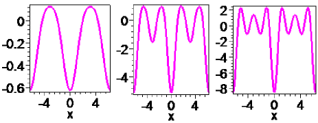
Figure 1. The designed optical super-lattice potentials(New Example 1) with period $2\pi$.

New Example 2: Multi-well potentials According to transformation eq.(3), we have got three types of multi-well potentials: 1) Let $a>0$, then $F(x)=\dfrac{1}{200}\dfrac{1}{\cos({\rm arccot}((x/20)^{2}+a))}$ gives symmetric double well potentials, which are plotted in Figure 2(left) for $a=0.001,0.2$ and $1$; 2)Let $a>0$, then $F(x)=((\dfrac{x}{30})^{4}+a(\dfrac{x}{50})^{2}+(\dfrac{x}{80})+4)/400$ gives non-symmetric double well potentials, which are plotted in Figure 2(middle) for $a=1/15,2$ and $7$. Note that the last one is a single well potential. 3) $F(x)=\dfrac{1}{15}\dfrac{1}{2\cos(4{\rm sech}(\frac{x}{20}))+1.3\cos({\rm sech}(\frac{x}{20}))+10}$ gives triple well potential, which is plotted in Figure 2(right).

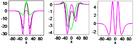
Figure 2. The designed multi-well potentials(New Example 2). Left panel(the symmetric double well potentials): From the thinnest(magenta) to the thickest(green) curves it denotes potential generated by $F(x)$ with $a=0.001,0.2,1$, respectively. Middle panel(the non-symmetric double well potentials): From the thinnest(magenta) to the thickest(green) curves it denotes potential generated by $F(x)$ with $a=1/15,2,7$,respectively. Right panel:the triple well potential.

Note that the associated other two coefficients $o(x,t)$ and $g(x,t)$ are given simultaneously by means of transformation eq.(3), such that VCNLSEs associated with these designed coefficients $o,g$ and $v$ are integrable systems. To save space, we do not write out them here. Moreover, double well potential can be achieved by taking $F(x)=0.35x^{2}+5{\rm sech}^{2}(0.27x)$. Additionally, by setting arbitrary functions in transformation eq.(3), the interested readers can design different integrable VCNLSE to establish mathematical model equation of physical systems. For instance, time-dependent optical super-lattice potential[44] can also be designed by setting $T=\int f(t)dt$ and $F(x)=1/(a\cos(x)+b)$ in $v(x,t)$. Here $b>a>0$.

Furthermore, the transformation eq.(3) provides an efficient way to construct exact and analytic solutions $\psi(x,t)$ of the designable VCNLSE from known solutions $q(X,T)$ of the NLSE, such that we can explore the dynamical evolution of solitons of the VCNLSE conveniently. For example, setting a usual single soliton $q(X,T)$ as

$$|q(X,T)|=\frac{2\sqrt{2}|\eta_{1}|}{\cosh(2\eta_{1}\sqrt{2}X+8\eta_{1}\xi_{1}T)},$$ (25)

which is given by eq.(6) of reference [24]. Obviously, the profile of the usual soliton $q(X,T)$ on the plane of (X,T) is invariant when soliton evolves with time $t$. A single soliton of the VCNLSE,

$$|\psi(x,t)|=|p(x,t)||q(X,T)|=|p(x,t)|\frac{2\sqrt{2}|\eta_{1}|}{\cosh(2\eta_{1}\sqrt{2}X+8\eta_{1}\xi_{1}T)},$$ (26)

is obtained by using transformation eq.(3). Note that the profile of the soliton $|\psi(x,t)|$ of the VCNLSE is not preserved when it evolves with time $t$ because the amplitude $|p(x,t)|$ is a function of $x$ and $t$ and the trajectory is a curve $x=x(t)$ on the plane of (x,t), which is defined implicitly by

$$\sqrt{2}X(x,t)+4\xi_{1}T(t)=0.$$ (27)

This shows that the profile of the soliton of the VCNLSE is designable by using different $p(x,t)$, $X(x,t)$ and $T(t)$, which can be realized by choosing different arbitrary functions $f_{1}(t),f_{3}(t),F(x)$ and $T(t)$ in transformation eq.(3). In particular, as we shall show in the following example, the amplitude of $\psi(x,t)$ is dependent of $t$ even if the $p=p(x)$ is x-dependent only, because $p=p(x(t))$ when soliton moves along the trajectory $x=x(t)$.

To further illustrate the property of dynamical evolution of the soliton $|\psi(x,t)|$ of the VCNLSE, one example is given here. According to the above formula eq.(26), the solution of the case 1) in New Example 1 is a deformed single soliton,i.e.,

$$|\psi(x,t)|=\dfrac{2|\eta 1|}{\sqrt{\dfrac{1}{2\cos(x)+3}}\cosh\Big{(}2\sqrt{2}\eta_{1}\widetilde{X}+8\xi_{1}\eta_{1}t\Big{)}},$$ (28)

which is plotted in Figure 3 with $\xi_{1}=0.1$ and $\eta_{1}=-0.1$.

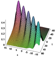
Figure 3. The dynamical evolution on ($x-t$) plane of a single soliton of the VCNLSE with an optical super-lattice potential designed by case 1) of New Example1.

Here $\widetilde{X}=\dfrac{4}{\sqrt{5}}\big{(}\arctan(\dfrac{1}{\sqrt{5}}\tan(\dfrac{x}{2}))+\big{[}\dfrac{\frac{x}{2}+\frac{\pi}{2}}{\pi}\big{]}\pi\big{)}+1$, and $\big{[}x\big{]}$ is the greatest integer less than or equal to $x$. Particularly, $\widetilde{X}$ is a monotonically increasing and continuous function of $x$, which is obtained from eq.(6) by adding the floor function $\big{[}x\big{]}$. Figure 3 shows intuitively two interesting features of the soliton of the VCNLSE: 1) the profile is variable and 2) the trajectory is not a straight line when it evolves with time $t$, as we pointed in the above paragraph. This is also supported visibly by Fig.4 for profiles of different time $t$ and Fig 5 for the trajectory on the plane of (x,t), which is given by $\sqrt{2}\widetilde{X}+0.4t=0.$

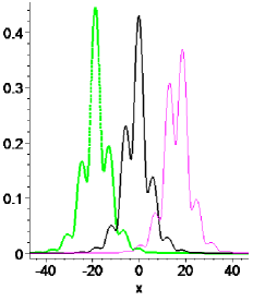
Figure 4. The one-dimensional profiles of single soliton in Fig.3 at different times. From the right(magenta) to the left(green) curves it denotes soliton at $t=-55,0,55$, respectively.

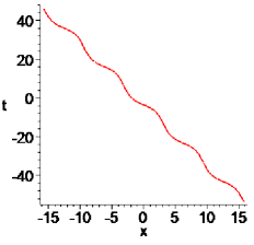
Figure 5. Trajectory of the single soliton in Fig 3.

Note that there are many other kinds of solutions of NLSE, such as dark soliton, periodic solution, position, negation, complexiton, etc., which can be used to generate the solutions of the VCNLSE. In ourexamples, merely the single bright soliton of the NLSE is used. Especially, from the “seed” of the multi-soliton solutions of NLSE, the multi-soliton solutions of the VCNLSE can be obtained, and then its interaction properties are discussed. However, it is very difficult to find multi-soliton solutions of the VCNLSE from the view of non-isospectral integrable system.

5. Conclusions

In conclusion, a new concept “designable integrability ”[40] of the VCNLSE has been developed by a novel transformation eq.(3). The novel characteristic of VCNLSE with DI is that the variable coefficients with physical meaning including $o(x,t),v(x,t)$ and $g(x,t)$ can be designed artificially and analytically according to different physical considerations. Correspondingly, the profile of its solutions including soliton and others are also tunable intentionally by using different $p(x,t)$, $X(x,t)$ and $T(t)$, which can be realized by choosing different arbitrary functions. The nonautonomous NLSE[8] is re-obtained as a special design through choosing $F(x)=F_{0}$(constant). Furthermore, two kinds of NEW VCNLSE with optical super-lattice potentials and multi-well potentials have been designed respectively, and two interesting features of the soliton of the VCNLSE are shown by formulas and figures. The results in this paper show that DI and some unusual behaviors of solitons for the VCNLSE originate from the usual NLSE and the transformation eq.(3). The methodology of studying variable coefficients partial differential equations with DI can be extended to many other cases including other (1+1)-dimensional, even higher dimensional integrable systems, multi-component systems and discrete systems. In particular, the method to design the solvable $o$, $v$ and $g$ of the VCNLSE is expected optimistically to be used by theoretical and experimental researchers.

As the end of this paper, the method applied to a more general VCNLSE

$$i\dfrac{\partial}{\partial t}\psi(x,t)+\frac{1}{2}o\dfrac{\partial^{2}}{\partial x^{2}}\psi(x,t)-v\psi(x,t)-g|\psi(x,t)|^{2}\psi(x,t)-i\Gamma\psi(x,t)=0,$$ (29)

which is a minor extension of modeling equations of BECs and nonlinear optics in recent many works,is shown here. In order to guarantee integrability of eq.(29), Luo et al have shown that $o,g,\Gamma$ must be time-independent, and $v(x,t)$ must be a second order polynomial of $x$ and satisfy a integrable condition (eq.(22) of reference[28]). However, their integrable conditions are too strong because of the restriction of the Painleve analysis, and a very general forms of $o,g,v$ , which are real functions of $x$ and $t$, has been achieved by a similar transformation of eq.(3). This provide us more possibility for soliton control, which will be given in a separate paper.

Acknowledgments

This work is supported by the NSF of China under Grant No.10671187 and 10971109. Jingsong He is also supported by Program for NCET under Grant No.NCET-08-0515. Yishen Li is supported by NSF of China under Grant No.10971211. We express our sincere thanks to Dr. Chaohong Li and Xiwen Guan for their helpful discussion on early results at Nov. 2007(ANU,Canberra), and Prof. Wuming Liu for his suggestions at Sept. 2008(USTC,Hefei) and at Oct.2008(IOP,Beijing). Jingsong He thanks Prof. Jiefang Zhang(ZJNU,China) for his useful suggestions at Oct. 2009(NBU,China) on the optical lattice potentials. Many thanks to Mr. Xiaodong Li, Mr. Jipeng Cheng and Ming Gong(USTC,Hefei) for their helps. The transformation eq.(3) and its special case eq.(24) in this paper was presented orally by Li at “Integrable System” session, International Conference: Nonlinear Waves(Beijing, China, June 9-12,2008)(unpublished). We thank anonymous referee for his/her valuable suggestions and criticisms on the profile of single soliton.

References

- [1] H. H. Chen, and C. S. Liu,Solitons in Nonuniform Media, Phys. Rev. Lett.37:693-697(1976).
- [2] F. Calogero and A. Degasperis,Extension of the Spectral Transform Method for Solving Nonlinear Evolution Equations, Lett. Nuovo Comento 22:131-137(1978); Extension of the Spectral Transform Method for Solving Nonlinear Evolution Equations. II , ibid.22: 263-269(1978).
- [3] A. Newell,The general structre of integrable evolution equations, Proc. R. Soc. Lond. A. 365:283-311(1979).
- [4] Y.S. Li and G. C. Zhu,New set of symmetries of the integrable equations, Lie algebra and nonisospectral evolution equations. II. AKNS system,J. Phys. A19: 3713-3725(1986).
- [5] N.Akhmediev and A. Ankiewicz, Solitons, Nonlinear Pulses and Beams,Chapman & Hall, London,1997; Dissipative Solitons,Springer-Verlag, Berlin,2005.
- [6] Yu.S. Kivshar and G. P. Agrawal, Optical Solitons: From Fibers to Photonic Crystals( Academic Press, San Diego, 2003).
- [7] V. N. Serkin and A. Hasegawa,Novel Soliton Solutions of the Nonlinear Schröinger Equation Model,Phys. Rev. Lett. 85:4502-4505(2000).
- [8] V. N. Serkin, A. Hasegawa, and T. L. Belyaeva,Nonautonomous Solitons in External Potentials, Phys. Rev. Lett. 98:074102(2007).
- [9] V.I.Kruglov, A.C.Peacock, and J. D. Harvey,Exact Self-Similar Solutions of the Generalized Nonlinear Schrödinger Equation with Distributed Coefficients, Phys.Rev.Lett.90:113902(2003).
- [10] S. A. Ponomarenko and G. P. Agrawal,Do Solitonlike Self-Similar Waves Exist in Nonlinear Optical Media?, Phys. Rev. Lett. 97:013901(2006).
- [11] V. V. Konotop and P.Pacciani,Collapse of Solutions of the Nonlinear Schrödinger Equation with a Time-Dependent Nonlinearity: Application to Bose-Einstein Condensates, Phys. Rev. Lett. 94:240405(2005).
- [12] J. Belmonte-Beitia, V. M. Perez-Garcia,V. Vekslerchik, and P. J. Torres, Lie Symmetries and Solitons in Nonlinear Systems with Spatially Inhomogeneous Nonlinearities, Phys. Rev. Lett. 98:064102(2007)
- [13] J. Belmonte-Beitia, V. M. Perez-Garcia, V. Vekslerchik, and V. V. Konotop, Localized Nonlinear Waves in Systems with Time- and Space-Modulated Nonlinearities, Phys. Rev. Lett. 100:164102(2008).
- [14] H. Saito and M. Ueda, Dynamically Stabilized Bright Solitons in a Two-Dimensional Bose-Einstein Condensate, Phys. Rev. Lett. 90:040403(2003).
- [15] Z. X. Liang, Z.D. Zhang,and W. M. Liang,Dynamics of a Bright Soliton in Bose-Einstein Condensates with Time-Dependent Atomic Scattering Length in an Expulsive Parabolic Potential, Phys. Rev. Lett. 94:050402(2005).
- [16] Y. Sivan, G. Fibich, and M. I. Weinstein,Waves in Nonlinear Lattices: Ultrashort Optical Pulses and Bose-Einstein Condensates, Phy. Rev. Lett. 97:193902(2006)
- [17] C.Sulem and P.L.Sulem, The Nonlinear Schrödinger Equations,Springer-Verlag, New York, 1999.
- [18] G. Theocharis, Z. Rapti, P. G. Kevrekidis, D.J. Frantzeskakis, and V.V. Konotop, Modulational instability of Gross-Pitaevskii-type equations in 1+1 dimensions, Phys.Rev. A 67:063610(2003).
- [19] L.Wu, J.F.Zhang, and L. Li, Modulational instability and bright solitary wave solution for Bose-Einstein condensates with time-dependent scattering length and harmonic potential, New J. Phys. 9:69(2007).
- [20] L.Wu, J.F.Zhang, L.Li,Q.Tian, and K.Porsezian,Similaritons in nonlinear optical systems, Opt.Express 16:6352-6360(2008).
- [21] V. M.Perez-Garcia, P. J. Torres, and V. V. Konotop,Similarity transformations for nonlinear Schrödinger equations with time-dependent coefficients, Physica D221:31-36(2006).
- [22] J. Belmonte-Beitia and Gabriel F. Calvo,Exact solutions for the quintic nonlinear Schröinger equation with time and space modulated nonlinearities and potentials, Phys. Lett. A373 :448-453(2009).
- [23] S. H. Chen and L. Yi,Chirped self-similar solutions of a generalized nonlinear Schröinger equation model, Phys. Rev. E71:016606(2005).
- [24] J. S. He, M. Ji, and Y.S. Li, Solutions of two kinds of non-isospectral generalized nonlinear Schrödinger equation related to Bose-Einstein Condensates,Chin. Phys. Lett. 24:2157-2160(2007).
- [25] H.M. Li, Y.S. Li, and J. Li,Abundant exact solutions for a strong dispersion-managed system equation, Chin. Phys. B 18:3657-3662(2009).
- [26] M. Gürses, Integrable nonautonomous nonlinear Schrödinger equations(arXiv:0704.2435v2).
- [27] D.Zhao, H.G. Luo, and H. Y.Chai,Integrability of the Gross-Pitaevskii equation with Feshbach resonance, Phys. Lett. A372:5644-5650(2008).
- [28] X.G.He, D.Zhao, L.Li, and H.G.Luo,Engineering integrable nonautonomous nonlinear Schröinger equations, Phys.Rev.E 79,056610(2009).
- [29] A. Kundu,Integrable nonautonomous nonlinear Schröinger equations are equivalent to the standard autonomous equation,Phys. Rev. E79,015601(R)(2009).
- [30] P.J.Louis, E.A. Ostrovskaya, C.M.Savage, and Y.S.Kivshar, Bose-Einstein condensates in optical lattices:Band-gap structure and solitons, Phys.Rev.A 67:013602(2003); P.J.Louis, E.A. Ostrovskaya, and Y.S.Kivshar,Matter-wave dark solitons in optical, J.Opt.B 6:S309-S317(2004); ibid., Dispersion control for matter waves and gap solitons in optical superlattices, Phys.Rev.A 71: 023612(2005).
- [31] S. K. Adhikari and B. A. Malomed,Tightly bound gap solitons in a Fermi gas, Eur.Phys. Lett.79:50003(2007); ibid.,Gap solitons in a model of a superfluid fermion gas in optical lattices,Physica D238:1402-1412(2009);
- [32] M.Salerno, V.V.konotop, and Yu.V.Bludov, Long-Living Bloch Oscillations of Matter Waves in Periodic Potentials,Phys. Rev. Lett. 101:030405(2008); Yu.V.Bludov, V.V.konotop, and M.Salerno, Long lived matter waves Bloch oscillations and dynamical localization by time dependent nonlinearity management, J. Phys. B.42:105302(2009) .
- [33] M. A. Porter, P.G. Kevrekidis, R. Carretero-Gonzlez, and D. J. Frantzeskakis, Dynamics and manipulation of matter-wave solitons in optical superlattices, Phys. Lett.A 352: 210-215(2006);R.Carretero-Gonzlez, D. J. Frantzeskakis, and P.G. Kevrekidis,Nonlinear waves in Bose-Einstein condensates: physical relevance and mathematical techniques,Nonlinearity 21:R139-R202(2008).
- [34] Y.P.Zhang and B.Wu, Composition Relation between Gap Solitons and BlochWaves in Nonlinear Periodic Systems,Phys. Rev. Lett. 102:093905(2009).
- [35] E.A. Ostrovskaya,Y.S.Kivshar,M. Lisak, B. Hall,and F. Cattani, Coupled-mode theory for Bose-Einstein condensates”,Phys.Rev.A 61:031601(R)(2000).
- [36] V. S. Shchesnovich, B.A.Malomed, and R.A. Kraenkel, Solitons in Bose-Einstein condensates trapped in a double-well potential, Physica D188:213-240(2004); T. Mayteevarunyoo, B. A. Malomed, and G.J.Dong, Spontaneous symmetry breaking in a nonlinear double-well structure, Phys. Rev.A 78: 053601(2008).
- [37] Y.Shin, M. Saba, A. Schirotzek, T. A. Pasquini, A. E. Leanhardt, D. E. Pritchard and W. Ketterle,Distillation of Bose-Einstein Condensates in a Double-Well Potential, Phys. Rev. Lett. 92:150401(2004);Y.Shin,G. B. Jo, M. Saba, T.A. Pasquini, W. Ketterle and D. E. Pritchard,Optical Weak Link between Two Spatially Separated Bose-Einstein Condensates,ibdi. 95:170402(2005).
- [38] D.R.Dounas-Frazer, A.M.Hermundstad,and L.D.Carr,Ultracold Bosons in a Tilted Multilevel Double-Well Potential,Phys. Rev. Lett. 99:200402(2007).
- [39] G. Theocharis, P.G. Kevrekidis, D. J. Frantzeskakis,and P.Schmelcher, Symmetry breaking in symmetric and asymmetric double-well potentials,Phys. Rev. E74: 056608 (2006); C.Wang,P.G. Kevrekidis,N.Whitaker, and B.A.Malomed, Two-component nonlinear Schrödinger models with a double-well potential,Physica D237:2922-2932(2008); C.Wang,P.G. Kevrekidis,N.Whitaker,T.J. Alexander,D. J. Frantzeskakis, and P.Schmelcher, Spinor Bose-Einstein condensates in double-well potentials, J. Phys. A42:035201 (2009).
- [40] A partial differential equation(PDE) I is said to be designable integrable if there exist an explicit transformation T with sevearl arbitrary functions mapping I to an integrable PDE II, such that the coefficients of I can be designed artificially and analytically by means of the selection of arbitrary functions according to different motivations. Here II is a well studied integrable PDE with non-variable coefficents. In contrast to I, II is called rigid integrable.
- [41] X. Q. Liu, S. Jiang, W. B. Fan, and W. M. Liu,Soliton solutions in linear magnetic field and time-dependent laser field, Commun. Nonlinear Sci. and Numer. Simul. 9:361-365(2004).
- [42] J. K. Xue, Controllable compression of bright soliton matter,J. Phys. B 38: 3841-3848(2005).
- [43] Q.Yang and J.F.Zhang, Bose-Einstein solitons in time-dependent linear potential, Optics Communications 258:35-42(2006).
- [44] D. Poletti,T. J. Alexander,E. A. Ostrovskaya, B.W. Li, and Y. S. Kivshar, Dynamics of Matter-Wave Solitons in a Ratchet Potential,Phys. Rev. Lett. 101, 150403(2008).