The dynamically induced Fermi arcs and Fermi pockets in two dimensions: a model for underdoped cuprates

Abstract

We investigate the effects of the dynamic bosonic fluctuations on the Fermi surface reconstruction in two dimensions as a model for the underdoped cuprates. At energies larger than the boson energy $\omega_{b}$, the dynamic nature of the fluctuations is not important and the quasi-particle dispersion exhibits the shadow feature like that induced by a static long range order. At lower energies, however, the shadow feature is pushed away by the finite $\omega_{b}$. The detailed low energy features are determined by the bare dispersion and the coupling of quasi-particles to the dynamic fluctuations. We present how these factors reconstruct the Fermi surface to produce the Fermi arcs or the Fermi pockets, or their coexistence. Our principal result is that the dynamic nature of the fluctuations, without invoking a yet-to-be-established translational symmetry breaking hidden order, can produce the Fermi pocket centered away from the $(\pi/2,\pi/2)$ towards the zone center which may coexist with the Fermi arcs. This is discussed in comparison with the experimental observations.

I Introduction

The “Fermi arc” picture was advanced by the angle-resolved photo-emission spectroscopy (ARPES) to understand the enigmatic pseudo-gap state in the underdoped cuprates.Marshall et al. (1996); Norman et al. (1998); Shen et al. (2005); Kanigel et al. (2006) The ARPES, with its momentum resolution capability, established that in this pseudo-gap state the gapped region is mainly in the $(0,\pi)$ and $(\pi,0)$ region while the Fermi surface (FS) exists in the diagonal direction. Then, the picturesque view of the pseudo-gap state is that the gapless portion of the FS forms an open ended arc, rather than a closed loop as in ordinary metals. It is extremely difficult to understand the abrupt truncation of the FS in the Brillouin zone. The Fermi arc has thus puzzled the physics community and triggered enormous research efforts.Timusk and Statt (1999)

This Fermi arc picture was challenged by the observations of the quantum oscillation under the applied magnetic field $H$.LeBoeuf et al. (2007); Sebastian et al. (2008); Doiron-Leyraud et al. (2007) The transport and thermodynamic properties exhibit the periodic oscillations as a function of the inverse magnetic field. The standard interpretation is in terms of the closed loop of the FS, or, the Fermi pockets. The oscillation is due to the quantizated Landau levels, and its periodicity is proportional to the area of the Fermi pocket. It is found to be only a few percent of the FS area of optimally or overdoped cuprates. In the theory of usual metals, such a small FS would require a change of translational symmetry from overdoped to underdoped cuprates. The problem is that there is no direct experimental evidence for the translational symmetry breaking for the compounds exhibiting the small FS. Moreover, the Fermi pocket is at odds with the Fermi arc picture from ARPES. Although the ARPES were done above $T_{c}$ with no magnetic field and the quantum oscillations in the low $T$ and strong external field, the views they advance, the Fermi arc and Fermi pocket, seem contradictory each other and need to be reexamined.

The recent laser ARPES on the single layer Bi₂Sr_2-xLa_xCuO₆ compounds by Meng $et~{}al.$ Meng et al. (2009) is indeed very interesting in this regard. They observed, with the improved resolution, that the ungapped portion of FS forms a closed loop, $e.g.$ the Fermi pocket, rather than the Fermi arcs at the doping levels of 11 and 12 % for Bi₂Sr_2-xLa_xCuO₆ . Moreover, the center of the Fermi pocket is shifted from the $(\pi/2,\pi/2)$ toward the zone center ($\Gamma$ point). The translational symmetry breaking, let alone its yet-to-be-established existence, can not explain their results because a salient feature of the reconstructed FS induced by the broken translational symmetry of period doubling is that the FS is symmetric with respect to the $(\pi,0)-(0,\pi)$ line.

Here, we wish to understand the Fermi pocket centered away from the $(\pi/2,\pi/2)$ point without invoking the translation symmetry breaking in terms of the $dynamic$ bosonic fluctuations. We first consider a dynamical collective mode coupled with quasiparticles at the antiferromagnetic (AF) wave vectors only (the correlation length $\xi\rightarrow\infty$) for simplicity and illustration of basic ideas. Then, the more realistic cases of finite $\xi$ are presented with self-consistent numerical calculations.

There have been many attempts to understand the Fermi arcs and pockets in the cuprates. Each of them has discrepancies with the experimental observations such as the shape, location, or the spectral weight.Wen and Lee (1996); Ng (2005); Yang et al. (2006); Norman et al. (2007); Sachdev et al. (2009); Greco (2009) On the other hand, the dynamic nature of the bosonic fluctuatoins peaked at $(\pi,\pi)$, without invoking a hidden order which breaks the translational symmetry, can produce the FS evolution from the large FS to Fermi arc to Fermi pocket as the coupling is increased. More specifically, it can induce (1) the Fermi pocket centered away from the $(\pi/2,\pi/2)$ towards the $\Gamma$ point, (2) the ratio of the spectral weight at the back side of the Fermi pocket to the inner side is about $10^{-2}$, (3) coexistence of the Fermi pocket and the large main FS, and (4) the dispersion kink along the nodal direction at energy $\approx 0.05$ eV. These are in agreement with the recent laser ARPES experiment of Meng $et~{}al$ Meng et al. (2009) and numerous previous experimental reports.Damascelli et al. (2003); Bogdanov et al. (2000); Kaminski et al. (2000); Lanzara et al. (2001)

After the bare band dispersion is determined there are three factors which affect the Fermi surface reconstructions: the fluctuations correlation length $\xi$, coupling constant $\alpha$, and the boson frequency scale $\omega_{b}$. More discussion about their possible microscopic origin and relation will made later in Sec. V in connection with other approaches. For now, we first take the Einstein mode of $\omega_{b}$ for simplicity. $\omega_{b}=0.05$ eV was chosen to match the kink energy.Bogdanov et al. (2000); Kaminski et al. (2000); Lanzara et al. (2001) We will also consider the realistic frequency dependent bosonic spectrum recently deduced by Bok $et~{}al$Bok et al. (2010) by inverting the laser ARPES on Bi₂Sr₂CaCu₂O_8+δ . We then perform detailed numerical calculations and show that the dynamic nature of the collective mode can account for the FS evolution without introducing a yet-to-be-established hidden order parameter.

II Idea and Formulation

We consider the renormalization of the fermions due to the coupling to the dynamic bosonic fluctuations $F({\bf q},\omega)$ with the coupling vertex $\alpha({\bf k},{\bf k}^{\prime})$. The self-energy of the fermion is given byKampf and Schrieffer (1990)

$$\Sigma({\bf k},\omega)=\int_{-\infty}^{\infty}d\epsilon\int_{-\infty}^{\infty}d\epsilon^{\prime}\frac{f(\epsilon)+n(-\epsilon^{\prime})}{\epsilon+\epsilon^{\prime}-\omega-i\delta}$$

$$\times\sum_{{\bf k}^{\prime}}A({\bf k}^{\prime},\epsilon)\alpha^{2}F({\bf k},{\bf k}^{\prime},\epsilon^{\prime}),$$ (1)

where $A$ is the spectral function of the fermion, and $f$ and $n$ are the Fermi and Bose distribution functions, respectively.

$$A({\bf k}^{\prime},\epsilon)=-\frac{1}{\pi}Im\frac{1}{\epsilon-\xi_{{\bf k}^{\prime}}-\Sigma({\bf k}^{\prime},\epsilon)},$$ (2)

$$\alpha^{2}F({\bf k},{\bf k}^{\prime},\epsilon^{\prime})=-\frac{1}{\pi}\alpha({\bf k},{\bf k}^{\prime})^{2}ImV({\bf k}-{\bf k}^{\prime},\epsilon^{\prime}).$$ (3)

We took the fluctuation spectrum of the following factorized form:Kampf and Schrieffer (1990)

$$\alpha^{2}F({\bf k},{\bf k}^{\prime},\epsilon^{\prime})=\alpha({\bf k},{\bf k}^{\prime})^{2}F(\epsilon^{\prime})$$

$$\times\sum_{{\bf Q}={\pm\pi/a,\pm\pi/a}}\frac{\Gamma/\pi}{(q_{x}-Q_{x})^{2}+\Gamma^{2}}\frac{\Gamma/\pi}{(q_{y}-Q_{y})^{2}+\Gamma^{2}},$$ (4)

where $a$ is the lattice constant, ${\bf q}={{\bf k}}^{\prime}-{{\bf k}}$, and $\Gamma=\pi/\xi$. The coupling $\alpha$ may depend on the wave vectors ${\bf k}$ and ${\bf k}^{\prime}$, but for simplicity we will consider a constant $\alpha$ and the Einstein model of frequency $\omega_{b}$ first.

$$\alpha^{2}F(\epsilon^{\prime})=\alpha^{2}\left[\delta(\epsilon^{\prime}-\omega_{b})-\delta(\epsilon^{\prime}+\omega_{b})\right].$$ (5)

Some remarks will be made on the more realistic frequency dependence of $F({\bf q},\epsilon^{\prime})$ and the momentum dependence of $\alpha({\bf k},{\bf k}^{\prime})$ later. Eqs. (II) and (2) constitute the coupled self-consistency equations. They are solved self-consistently for the self-energy via numerical iterations. A very similar problem was investigated by Grilli $et~{}al.$ for the one dimensional electronic systems.Grilli et al. (2009) It is extended to two dimensions in the present work fully self-consistently.

Let us first consider the simple case of $T\rightarrow 0$ and $\Gamma\rightarrow 0$ to gain underlying physics. That is, the boson mode is of a delta function in both the energy and momentum channels. Then, in the limit $T\rightarrow 0$, Eq. (II) is reduced to

$$\Sigma({\bf k},\omega)=-\alpha^{2}\int_{-\infty}^{\infty}d\epsilon\left[\frac{\Theta(\epsilon)}{\epsilon+\omega_{b}-\omega-i\delta}\right.$$

$$\left.+\frac{\Theta(-\epsilon)}{\epsilon-\omega_{b}-\omega-i\delta}\right]A({\bf k}_{Q},\epsilon),$$ (6)

$$Im\Sigma({\bf k},\omega)=-\pi\alpha^{2}\left[\Theta(\omega-\omega_{b})A({\bf k}_{Q},\omega-\omega_{b})\right.$$

$$\left.+\Theta(-\omega-\omega_{b})A({\bf k}_{Q},\omega+\omega_{b})\right],$$ (7)

where ${\bf k}_{Q}={\bf k}+{\bf Q}$ and $\Theta$ is the step function. A useful approximation is to take

$$A({\bf k},\epsilon)=\delta(\epsilon-\xi_{k}).$$ (8)

We then have

$$\Sigma({\bf k},\omega)=\alpha^{2}\left[\frac{\Theta(\xi_{k_{Q}})}{{\omega+i\delta-\xi_{k_{Q}}-\omega_{b}}}\right.$$

$$\left.+\frac{\Theta(-\xi_{k_{Q}})}{{\omega+i\delta-\xi_{k_{Q}}+\omega_{b}}}\right]=\frac{\alpha^{2}}{\omega+i\delta-\tilde{\xi}_{k_{Q}}},$$ (9)

with the definition

$$\tilde{\xi}_{k_{Q}}=\xi_{k_{Q}}+sgn(\xi_{k_{Q}})\omega_{b}.$$ (10)

The Green’s function of quasi-particle (qp) is given by

$$G({\bf k},\omega)=\frac{1}{\omega-\xi_{k}-\frac{\alpha^{2}}{\omega-\tilde{\xi}_{k_{Q}}}}.$$ (11)

This form of the Green’s function appeared previously in the context of the pseudogap.Yang et al. (2006); Sachdev et al. (2009) The coupling vertex $\alpha({\bf k},{\bf k}^{\prime})$ of present approach corresponds to the pseudogap $\Delta_{R}$ of Ref. Yang et al. (2006). It will be interesting to check to what extent this mapping is valid. An important distinction of the present approach is that the dynamics of the bosonic fluctuations is explicitly built in via $\tilde{\xi}_{k_{Q}}$ of Eq. (10). It is precisely this dynamics which gives rise to the Fermi arcs as we will see now.

The qp dispersion $E({\bf k})$ is determined by

$$G^{-1}({\bf k},\omega)=\omega-\xi_{k}-\Sigma({\bf k},\omega)=0,$$ (12)

which gives

$$E_{\pm}({\bf k})=\frac{1}{2}\left[\xi_{k}+\tilde{\xi}_{k_{Q}}\pm\sqrt{(\xi_{k}-\tilde{\xi}_{k_{Q}})^{2}+4\alpha^{2}}\right].$$ (13)

The results may approximately be extended to the case of finite correlation length $1/\xi\neq 0$ following Ref. Kuchinskii and Sadovskii (2008) by replacing the imaginary part of the frequency by $\delta=\hbar v_{F}/\xi$.

The Green’s function may be cast into the form

$$G({\bf k},\omega)=\frac{u_{k}^{2}}{\omega+i\delta-E_{+}}+\frac{v_{k}^{2}}{\omega+i\delta-E_{-}},$$ (14)

where the coherence factors are given by

$$u_{k}^{2}=\frac{1}{2}\left[1+\frac{\xi_{k}-\tilde{\xi}_{k_{Q}}}{\sqrt{(\xi_{k}-\tilde{\xi}_{k_{Q}})^{2}+4\alpha^{2}}}\right],$$

$$v_{k}^{2}=\frac{1}{2}\left[1-\frac{\xi_{k}-\tilde{\xi}_{k_{Q}}}{\sqrt{(\xi_{k}-\tilde{\xi}_{k_{Q}})^{2}+4\alpha^{2}}}\right].$$ (15)

The $E_{+}$ and $E_{-}$ represent, respectively, the electron and hole bands. The spectral function $A({\bf k},\omega)$ is then

$$A({\bf k},\omega) = -\frac{1}{\pi}ImG({\bf k},\omega)$$ (16)

$$= u_{k}^{2}\delta(\omega-E_{+}({\bf k}))+v_{k}^{2}\delta(\omega-E_{-}({\bf k})).$$

The spectral function is directly probed by the ARPES.

III Preliminary analysis

Before showing the detailed numerical results, we will first present the preliminary analysis to gain underlying physics of the problem. The bare dispersion of Bi₂Sr_2-xLa_xCuO₆ is taken as

$$\xi_{k} = -2t[\cos(k_{x}a)+\cos(k_{y}a)]+4t^{\prime}\cos(k_{x}a)\cos(k_{y}a)$$ (17)

$$- 2t^{\prime\prime}[\cos(2k_{x}a)+\cos(2k_{y}a)]-\mu,$$

where $t=0.25,~{}t^{\prime}=0.058,~{}t^{\prime\prime}=t^{\prime}/2$ eV.Hashimoto et al. (2008) The FS corresponding to the $\xi_{k}$ and $E_{\pm}({\bf k})$ with $\alpha=0.1$ eV, $\omega_{b}=0.05$ eV, and $\mu=-0.208$ eV corresponding to the slight underdoping of 12 % are shown in Fig. 1. The nodal cut of $k_{x}=k_{y}$ and several cuts parallel to it are also shown with dashed lines.

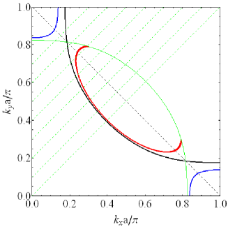
Figure 1: The reconstructed FSs for $\omega_{b}=0.05$, $\alpha=0.1$, and $\mu=-0.208$ eV corresponding to $x=12$ % doping. The thick black curve is the bare FS determined by $\xi_{k}=0$ of Eq. (17) and the green curve is the shadow FS of $\xi_{k+Q}=0$. The red curve around the $(\pi/2,\pi/2)$ point shows the hole FS of $E_{-}({\bf k})=0$. Notice that the outer portion is gapped and the hole FS forms the Fermi arc. The blue curves around $(0,\pi)$ and $(\pi,0)$ are the electron FS of $E_{+}({\bf k})=0$. As $\alpha$ increases it may disappear as shown in Fig. 3. The nodal cut of $k_{y}=k_{x}$ and the parallel cuts of $k_{y}=k_{x}+0.1n$ with $n=1-7$ are indicated with dashed green lines. The band dispersions along these cuts are shown in Fig. 2.

Along the cuts the qp dispersions are presented in Fig. 2 to better reveal the dynamically generated gap close to the shadow FS. Fig. 2(a) is the hole band dispersion $E_{-}({\bf k})$ in solid blue and electron band $E_{+}({\bf k})$ in dashed green lines along the nodal cut given by Eq. (13). The important point is that the hole band dispersion exhibits the abrupt jump at $k_{x}a/\pi\approx 0.6$, or the gap of about 2$\omega_{b}$. The dynamically induced gap was noticed by Grilli $et~{}al.$ for the one dimensional electronic systems.Grilli et al. (2009)

The gap of $2\omega_{b}$ means that for $\omega=0$ there exists only a single ${\bf k}$ point which satisfies $\omega=E_{-}({\bf k})$, while for $|\omega|\gtrsim\omega_{b}$ there exist two ${\bf k}$ points, one close to the original FS and the other to the shadow FS. That is, the shadow feature is present for $|\omega|\gtrsim\omega_{b}$, but is absent for $\omega=0$. This is in accord with general expectations: A physical system may have long (but finite) ranged order-parameter spatial correlations which fluctuate with the frequency $\omega_{b}$. The system then appears to be ordered above $\omega_{b}$. For energies larger than $\omega_{b}$ with respect to the Fermi energy the spectra should resemble an ordered system. On the other hand, at lower energies electrons “sense” averaged order-parameter fluctuations, and the system appears to be not disturbed much from the one without the collective mode.

The blowup of the hole band dispersions is shown in Fig. 2(b) along the cuts parallel to the nodal cut. Notice that the gap survives beyond $k_{y}a/\pi=k_{x}a/\pi+0.4$. It simply means that the gapless portion of the FS forms an open ended arc as shown with the thick red solid curve in Fig. 1. We stress that the abrupt truncation of the FS, which seemed so puzzling, is naturally understood in terms of the dynamic boson mode.

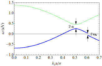
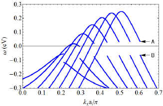
Figure 2: The hole and electron band dispersions, $E_{-}({\bf k})$ and $E_{+}({\bf k})$, along the cuts parallel to the nodal cut indicated with the green dashed lines in Fig. 1 with the same parameters. Fig. 2(a) shows the hole band in solid blue and electron band dispersion in dashed green curve along the nodal cut. Notice that the hole band dispersion has a gap of $2\omega_{b}$ at $k_{x}a/\pi\approx 0.6$. The detailed hole band dispersions are plotted in Fig. (b) along the cuts of $k_{y}a/\pi=k_{x}a/\pi+0.1n$ with $n=0-6$ from right to left. The gap survives beyond $k_{y}a/\pi=k_{x}a/\pi+0.4$. It means that the gapless portion of the FS forms an open ended arc as shown with the thick red solid curve in Fig. 1.

Fig. 3 is the 3D plot of the spectral function $A({\bf k},\omega)$ as a function of ${\bf k}$ at $\omega=0$. Fig. 3(a) is for $\omega_{b}=0.05$ eV, $\alpha=0.1$ eV, and $x=12$ %. Because of the dynamically generated gap close to the shadow FS discussed above, the spectral peak shows up only over a part of the FS instead of a closed loop as in Fig. 3(b). Also the spectral peaks from the electron band show up around $(0,\pi)$ and $(\pi,0)$ for a weak $\alpha$. Now, the FS may evolve to the Fermi pocket as the coupling $\alpha$ is increased. As an illustration, Fig. 3(b) is the 3D plot of the spectral function for $\alpha=0.2$ eV with all other parameters fixed. The Fermi pocket is clearly formed. The peaks from the electron band are substantially reduced. Physics behind the Fermi arc/Fermi pocket induced by the dynamic fluctuations is quite simple: The self-energy correction given by Eq. (II) dynamically generates a gap close to the shadow FS of magnitude of about $2\omega_{b}$, marked by “$2\omega_{b}$” in Fig. 2(a). As $\alpha$ increases, the gap between the electron and hole bands marked with “$2\alpha$” in Fig. 2(a) becomes larger and the hole dispersion $E_{-}({\bf k})$ of Eq. (13) is pushed down. Consequently, the qp states above the $2\omega_{b}$ marked with “A” in Fig. 2(b) touch the FS. Then FS forms over a closed loop, which is the Fermi pocket.

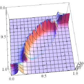
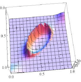
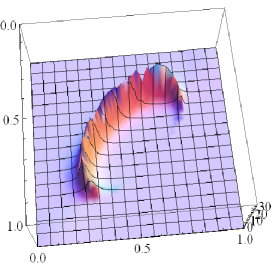
Figure 3: 3D plot of the spectral function $A({\bf k},\omega=0)$. Fig. (a) is for $\omega_{b}$=0.05, $\alpha=0.1$, and $\mu=-0.208$ eV corresponding to $x=12$ %. The Fermi arc appears because of the dynamically generated gap of magnitude of $2\omega_{b}$ close to the shadow FS. For Fig. (b), the parameters are the same as Fig. (a) except $\alpha=0.2$. The Fermi pocket appears now because the gap is pushed down below the Fermi energy. Fig. (c) is for $|\alpha({\bf k},{\bf k}^{\prime})|^{2}=\alpha_{0}^{2}\left|{\bf k}\times{\bf k}^{\prime}\right|^{2}$ with $\alpha_{0}=0.3$ and all other parameters the same as (b). The formation of the Fermi pocket is less favored.

Where $E_{-}({\bf k})=0$ either Fermi arc or Fermi pocket shows up. If two ${\bf k}$ points satisfy $E_{-}({\bf k})=0$ along any cut between the two hot spots and parallel to the nodal cut, then the Fermi pocket is produced. If, on the other hand, either one or two ${\bf k}$ points satisfy $E_{-}({\bf k})=0$, then a portion of a pocket is missing, which is just the Fermi arc. Both cases can be produced with the simple formula of Eq. (16) depending on the parameters as discussed above.

Also interesting is the relative weights of the two peaks of the Fermi pocket. For example, along the nodal cut, there appear two peaks near the main band and shadow band as a function of the momentum amplitude. The ratio of the spectral weight on the back side of the pocket to that on the main FS is from Eq. (II)

$$\frac{v_{k}^{2}(\xi_{k_{Q}}=0)}{v_{k}^{2}(\xi_{k}=0)}\approx 2\left(\frac{\alpha}{\xi_{k_{Q}}}\right)_{\xi_{k}=0}^{2}\sim 0.01$$ (18)

in accord with the experimental observation.Meng et al. (2009)

We also considered the momentum dependent coupling $\alpha({\bf k},{\bf k}^{\prime})$ as suggested by Varma and coworkersVarma (2006); Aji et al. (2010) and also by Yang $et~{}al$.Yang et al. (2006)

$$|\alpha({\bf k},{\bf k}^{\prime})|^{2}=\alpha_{0}^{2}\left|{\bf k}\times{\bf k}^{\prime}\right|^{2}.$$ (19)

This form of coupling will modify the qp disperion less along the nodal cut because ${\bf k}\times{\bf k}^{\prime}\approx 0$ there. The Fermi pocket formation is less favored. In Fig. 3(c), we show $A({\bf k},\omega=0)$ for $\alpha_{0}=0.3$ eV with all other parameters the same as Fig. 3(b). The Fermi arcs are formed instead of the Fermi pocket as anticipated.

From the shapes of the Fermi arcs shown in Figs. 1 and 3, one may notice that the arcs turn in near the ends. It means that the Fermi arcs seem to deviate from the underlying FS near the ends. Norman $et~{}al.$ argued that this is a generic feature of the pseudogap induced by ${\bf q}\neq 0$ order parameters.Norman et al. (2007) This point seems to apply to the Fermi arcs induced by dynamic fluctuations as well although the turning in looks weaker.

Now we understood the basic physics underlying the Fermi arc and Fermi pocket formation with the simple dynamic bosonic fluctuations of $\omega_{b}=0.05$ eV and $\xi=\infty$. But, as $\xi\rightarrow\infty$ the boson mode must get soft and approach $\omega_{b}\rightarrow 0$. This relation was not satisfied in the simple case just presented. We therefore performed the full self-consistent calculations in the following section with finite $\xi$ and temperature. The important message of the numerical calculations will be that the dynamically generated gap of $2\omega_{b}$ in the back-side of the pocket as shown in Fig. 2(a) remains intact as can be seen from Fig. 4(a). It means that the qualitative feature of the FS evolution from the large FS to Fermi arcs to Fermi pockets is unaffected. This is easy to understand. The magnitude of discontinuity being determined by $\omega_{b}$, it is insensitive to $\xi=\infty$ or not as presented in the following section.

IV Numerical results

The previous discussion is based on approximate solution of the self-energy of Eq. (8). Although the approximation permits the simple and useful results discussed in the previous section, some of the results may be an artifact of the approximation. We therefore performed the full self-consistent calculations via numerical iterations of the coupled equations of Eqs. (II) and (2). We considered the finite correlation length ($\Gamma=\pi/\xi\neq 0$ in Eq. (4)) and non-zero temperature. The more realistic frequency dependent $\alpha^{2}F(\epsilon^{\prime})$ as extracted by Bok $et~{}al.$Bok et al. (2010) is also considered. The important effects of the self-consistency are that (a) the Fermi arc and Fermi pocket coexist and (b) the center of the Fermi pocket gets displaced towards the zone center. The fine details are determined by the parameters like $\alpha$, $\Gamma$, and $T$. The non-zero $\Gamma$, non-zero temperature, or the frequency distribution of $\alpha^{2}F(\epsilon^{\prime})$ smear the fine structures out.

It is interesting to note that the laser ARPES experiments observe that the Fermi pocket coexist with the Fermi arc. The coexistence may be understood as follows: Let us fist consider the hole FS. The electron FS follows the same arguments. The spectral function of Eq. (16) indicates that the peaks show up as a function of ${\bf k}$ where $E_{-}({\bf k})=0$ or $v_{k}^{2}$ is maximum for the hole FS. The reconstructed hole FS may appear in the region where $\xi_{k}>0$ and $\xi_{k+Q}>0$ around the $(\pi/2,\pi/2)$ point. The loci of maximum $v_{k}^{2}$ can be seen most clearly in the limit $\alpha=0$. Inspection of the coherence factor $v_{k}^{2}$ of Eq. (II) in the limit $\alpha=0$ reveals that $v_{k}=1$ for $\xi_{k+Q}>\xi_{k}$. Simultaneously, $E_{-}(k)$ needs to be close to 0 as the delta function of Eq. (16) requires. Both conditions are satisfied where $\xi_{k}=0$. It is expected that peaks are produced close to the original FS due to the $v_{k}^{2}$ factor of Eq. (II).

The coexistence may also be understood as follows: The so-called two-pole approximation of Eq. (8) produces two qp branches. Next order approximation, the three-pole approximation, is to use Eq. (16) to the self-energy. It produces three qp branches. Straightforward calculations reveal that, along the nodal cut near $\omega=0$ for example, there exist one branch close to the bare FS, and two branches almost symmetric around the $(\pi/2,\pi/2)$ at $(\pi/2\pm\epsilon,\pi/2\pm\epsilon)$. Between the two, the one closer to the bare FS, $(\pi/2-\epsilon,\pi/2-\epsilon)$, merges with the branch near the bare FS to form the main FS, and the one at $(\pi/2+\epsilon,\pi/2+\epsilon)$ forms the back side of the Fermi pocket. The self-consistent calculations to be presented below maintain this feature to produce the coexisting Fermi arcs and pockets.

Another effect of finite $\xi$ is to exhibit the dispersion kink near $\omega\approx\ -\omega_{b}$. In the limit of $\xi\rightarrow 0$, it is simple to see that

$$\Sigma({\bf k},\omega)=\alpha^{2}\ln\left|\frac{\omega_{b}-\omega}{\omega_{b}+\omega}\right|.$$ (20)

Then, the slope of the qp dispersion changes from $1+2\alpha^{2}/\omega_{b}$ to 1 as $\omega$ increases past $\omega_{b}$. This dispersion kink along the nodal cut was observed by many groups and has been the focus of intense debate.

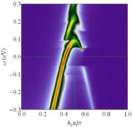
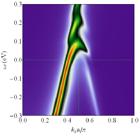
Figure 4: The qp dispersion along the nodal cut from the self-consistent calculation. $\alpha=0.18$ eV, $\Gamma=0.02$, and $T=0$ for Fig. (a) and $T=200$ K for Fig. (b). In the ARPES experiments the features above $\omega=0$ are cut off by the Fermi distribution function. Notice that the gap of $2\omega_{b}$ opens up in the back side of the pocket for $1/\xi\neq 0$ as well. Also notice the shadow feature around $\omega=0$ induced by the finite temperature effects. The shadow band disperses away from the zone center in accord with the observation by Meng $et~{}al.$

For finite $\xi$, the summation over ${\bf k}^{\prime}$ in Eq. (2) is not a delta function. The ${\bf k}^{\prime}$ summation was performed by using the 2D FFT (fast Fourier transform) between the momentum and real spaces using the convolution relation

$$\sum_{{\bf k}^{\prime}}F({\bf k}^{\prime}-{\bf k})G({\bf k}^{\prime})=F({\bf r})G({\bf r}).$$ (21)

$2^{8}$ points were taken for the FFT along each axis. For $\alpha$ not too large a convergence took about 10 iterations. For $\alpha$ larger than about 0.22 eV the procedure failed to converge in our numerical iterations. This could be an indication of a topological change of the Fermi surface.

Fig. 4 is the density plot of the spectral function $A({\bf k},\omega)$ along the nodal cut as a function of $k_{x}a/\pi$ and $\omega$ with $\alpha=0.18$ eV, $\Gamma=0.02$, and $T=0$ for (a) and $T=200$ K for (b). At $T=0$ the shadow band appears with the gap of $2\omega_{b}$ centered around the Fermi energy. The main band is modulated by the $\omega_{b}$ and the gap of $2\alpha$ is not distinguishable. The dispersion modulation, being determined by the energy $\omega_{b}$ in the case of the Einstein mode, is expected to be weakened if the spectrum has a finite energy distribution. This expectation is indeed the case as will be presented below in Fig. 7. Also noteworthy is that the shadow band disperses away from the $(\pi/2,\pi/2)$ as the energy is lowered in accord with the ARPES observation of Meng $et~{}al.$ Compare with the lower row of the plots b–d of the Fig. 1 in the Ref. Meng et al. (2009).

An important role of the finite temperature presented in Fig. 4(b) is to bring up the qp states $below$ the Fermi energy (marked by “B” in Fig. 2(b) for the two pole approximation) to form the Fermi pocket. This is in contrast with the simple results presented in the previous section. The non self-consistent preliminary analysis indicated that the qp states $above$ the Fermi energy (marked by “A” in Fig. 2(b)) are pushed down by the $\alpha$ and form the Fermi pocket. This picture is modified in the self-consistent calculations: As $\alpha$ increases the qp dispersion above the Fermi energy bends back as can be seen from Fig. 4(a) to keep the gap as intact as possible because the total energy will be lowered by not occupying the higher lying states. Instead the shadow band dispersion below the Fermi energy is extended above the Fermi energy to form a pocket as can be seen from Fig. 4(b). Note that at the Fermi energy the dispersion from below is closer to the zone center than the dispersion from above. Consequently, the pocket is displaced towards the zone center away from the $(\pi/2,\pi/2)$ point as shown in Fig. 5(a).

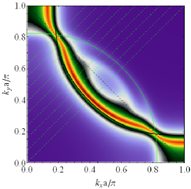
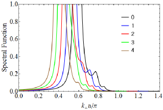
Figure 5: (a) The spectral function as a function of $k_{x}$ and $k_{y}$ at $\omega=0$ with the same parameters as the Fig. 4(b). The Fermi pocket is formed because of the temperature induced shadow feature around $\omega=0$. (b) The plots of the spectral function of (a) along the cuts parallel to the nodal cut. From right to left are the cuts of $k_{y}a/\pi=k_{x}a/\pi+0.2n$ with $n=0-4$.

In Fig. 5(a) we show the density plot of the spectral function $A({\bf k},\omega=0)$ as a function of ${\bf k}$ with the same parameters as the Fig. 4(b). Note the formation of the pocket coexisting with the main Fermi surface. The center of the pocket is shifted to the zone center away from the $(\pi/2,\pi/2)$ point as discussed above. Fig. 5(b) is the plots of the spectral function of $A({\bf k},\omega=0)$ along the cuts parallel to the nodal cut. From right to left are the cuts of $k_{y}a/\pi=k_{x}a/\pi+0.2n$ with $n=0-4$. Note the small peaks near the back side of the pocket. The ratio of their spectral weights to those on the main bands is found to be about $10^{-2}$.

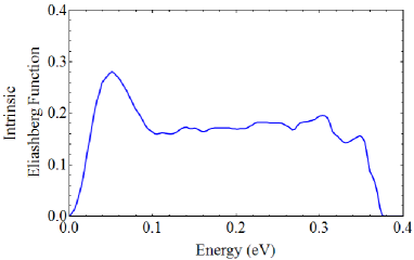
Figure 6: The input Eliashberg function taken from Bok $et~{}al$. The dimensionless coupling constant $\lambda\approx 1.5$. It corresponds, for the Einstein mode of $\omega_{b}=0.05$ eV, to $\alpha\approx 0.19$ eV.

We now turn to the realistic frequency dependent fluctuation spectrum. It was taken from Bok $et~{}al.$Bok et al. (2010) with a constant $\alpha$. The input Eliashberg function $\alpha^{2}F(\omega)$ is shown in Fig. 6. The extracted fluctuation spectrum has a peak around $\omega\approx 0.05$ eV, flattens out above 0.1 eV and has a cut-off at approximately 0.35 eV. The dimensionless coupling constant

$$\lambda=\int_{0}^{\infty}d\omega\frac{2\alpha^{2}F(\omega)}{\omega}$$ (22)

is $\lambda\approx 1.5$. The Eliashberg function $\alpha^{2}F(\theta,\omega)$ deduced by Bok $et~{}al.$, where $\theta$ is the tilt angle with respect to the nodal cut and $\omega$ is the energy, is that the functions along different angles collapse onto a single curve below the angle dependent cut-off energy $\omega_{c}(\theta)$. The cut-off is maximum along the nodal cut, $\omega_{c}\approx$ 0.35–0.4 eV, and decreases as the angle is increased. In the present calculations this angular dependence of the cut-off energy of the Eliashberg function was disregarded.

Eqs. (II), (2), and (4) were solved self-consistently via iterations taking the extracted $\alpha^{2}F$ of Fig. 6 into consideration. The ${\bf k}^{\prime}$ summation was performed using the 2D FFT as explained above. The finite range of the fluctuation spectrum instead of a delta function is to smear out fine structures of the spectral function as can be seen by comparing Fig. 7(a) with the Fig. 4 of a delta function fluctuation spectrum. In Fig. 7(a) we show the dispersion along the nodal cut at $T=100$ K, that is, the density plot of $A({\bf k},\omega)$ as a function of $k_{x}a/\pi$ and $\omega$. The shadow band is also smeared out and its width is increased as the energy is lowered. In Fig. (b) the density plot of $A({\bf k},\omega=0)$ is shown as a function of ${\bf k}$. The pocket becomes weaker compared with the delta function fluctuation spectrum of Fig. 5(a).

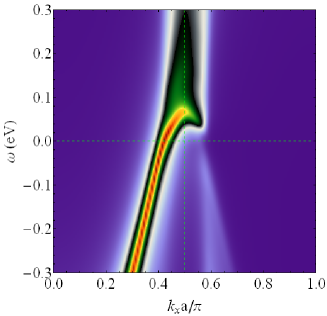
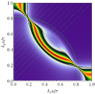
Figure 7: (a) The spectral function $A({\bf k},\omega)$ as a function of $k_{x}a/\pi$ and $\omega$ along the nodal cuts at $T=100$ K. The Eliashberg function of Fig. 6 was taken into consideration. (b) The 3D plot of $A({\bf k},\omega)$ as a function of ${\bf k}$ at $\omega=0$.

In order is to make a comment on implication of the coupling constant $\lambda$ of Eq. (22) on superconductivity. The approximate $T_{c}$ formula for $d$-wave superconductors is

$$T_{c}=\omega_{av}\ e^{-{(1+\lambda_{s})}/{\lambda_{d}}},$$ (23)

where $\lambda_{s}$ and $\lambda_{d}$ are the coupling constant in the normal and pairing channels, respectively. The $\lambda$ of Eq. (22) is $\lambda_{s}$ because it was extracted in the normal state. $T_{c}\sim 150$ K is produced if we take $\lambda_{d}=0.8\lambda_{s}$. This is in accord with the expectation $g=\lambda_{d}/\lambda_{s}<1$ for $d$-wave superconductors.Varma (2010)

V Remarks and outlook

We investigated the effects of the dynamic nature of bosonic fluctuations on the Fermi surface reconstruction as a model for the underdoped cuprates. The dynamic fluctuations induce the gap of magnitude $2\omega_{b}$ close to the shadow Fermi surface as Fig. 2 demonstrates. Then, the Fermi surface in momentum space can be truncated unlike the Fermi surface reconstruction induced by a long range order. Therefore, the Fermi arcs are naturally induced by the dynamic fluctuations. The Fermi arc and/or Fermi pocket is formed as Figs. 3, 5, and 7 show depending on the coupling constant $\alpha$ or the temperature $T$ or the correlation length $\xi$. The Fermi pocket is formed by the filling in of the dynamically generated gap by the non-zero temperature or the energy distribution of the bosonic spectrum $\alpha^{2}F(\omega)$. The self-consistency enables the Fermi arcs and pockets coexist and moves their center towards the zone center.

There have been many works along the same path adapted in this paper, namely, employing bosonic fluctuations to compute the renormalization of the electronic properties. See Ref. Varma (2010) for a recent review. Now, it will be in order to make some comments on and comparison with a few recent relevant works. In Ref. Greco (2009), Greco computed the electronic polarizability of $d$ density wave instability (or, flux phase) with the $t$-$J$ model. It was used as the bosonic fluctuations to couple to the electrons. The calculation is non-self-consistent and assumes the true phase transition of the flux phase. The symmetry broken phase, however, is yet to be confirmed experimentally. Nevertheless, Greco addressed some of the points we did not touch in this paper like the temperature dependence of the Fermi arc length.Kanigel et al. (2006) In the absence of any symmetry broken phase in the pseudogap doping range, however, we did not specify the mechanism of the boson mode in this paper. Instead we took a phenomenological effective interaction between electrons like Fig. 6. Because our main point was to demonstrate the Fermi surface evolution with $\alpha$, we did not pursue the questions like $T^{*}$, temperature dependence of the arc length, and so on, leaving them as further studies.

Dahm $et~{}al.$ made a check if a self-consistent description is possible between ARPES and inelastic neutron scattering (INS) for YBa₂Cu₃O_6.6.Dahm et al. (2009) In more detail, they fitted the INS to extract the spin susceptibility. Then they used it as the bosonic fluctuation to couple with the electrons to calculate the self-energy. The results were consistent with ARPES intensity and nodal dispersion, and the kink along the nodal cut was produced. This nodal kink is expected in their work because $\Gamma$ of the extracted susceptibility is non-zero.

The dynamic fluctuation model with no long-range order of the present paper successfully describes the FS evolution from the large FS to Fermi arc to Fermi pocket as the coupling is increased. Particularly, the enigmatic abrupt truncation of the FS can be naturally understood. Other satisfactory features include (a) the ratio of the spectral weight on the back side of the pocket to that on the main side, (b) the dispersion kink in the nodal direction around $\approx 0.05$ eV, and (c) the shadow band disperses out as the energy is lowered below the Fermi energy as Fig. 4(b) shows because the shadow feature is “reflection” of the main band with respect to the $(0,\pi)-(\pi,0)$ line. In the laser ARPES experiments by Meng $et~{}al.$ the shadow band was observed to disperse out as the binding energy increases. See the lower row of the plots b–d in the Fig. 1 of Ref. Meng et al. (2009).

Despite these satisfactory features of the dynamic fluctuations there are some discrepancies compared with experimental observations. First of all, the current scenario requires quite long correlation length of order of $\xi/a\sim 10$ for the Fermi arcs or Fermi pockets to appear. But, one of the present authors recently inverted the high resolution laser ARPES from Bi₂Sr₂CaCu₂O_8+δ  in pseudogap state to extract the bosonic fluctuations spectrum shown in Fig. 6. It was found that the correlation length is of the order of $\xi/a\lesssim 0.1$.Bok et al. (2010) Although the Eliashberg function was extracted in Bi₂Sr₂CaCu₂O_8+δ  and the Fermi pocket/arc was observed in Bi₂Sr_2-xLa_xCuO₆ , both experiments were carried out in the pseudogap state and this contradiction needs to be reconciled.

Secondly, if the fluctuation spectrum of Fig. 6 is peaked at $(\pi,\pi)$ with $\xi/a\sim 10$, then the transport $\lambda_{tr}\approx 2\lambda\approx 3$ in the nodal direction because of the $(1-\cos\theta)$ factor from the vertex correction. To our knowledge, this large $\lambda_{tr}$ was not observed in the resistivity measurements. Bok $et~{}al.$ concluded that the correlation length must be small, $\xi\ll a$, and the spectrum can not be from the $(\pi,\pi)$. The enhancement of $\lambda_{tr}$ over $\lambda$ is not expected. An interesting point in this context though is the observation by Schachinger and Carbotte.Schachinger and Carbotte (2008) They compared the $\alpha^{2}F$ from infrared (IR) spectroscopy and ARPES and found that they agree well overall (after scaling) except that $\alpha^{2}F$ from IR is larger than that from ARPES around 0.06 eV by the factor of approximately 2. This may be understood if the peak around 0.06 eV is dominantly from $(\pi,\pi)$ and the rest of the spectrum is momentum independent. However, this scenario seems to be at odds with the conclusion of Bok $et~{}al$.

As the coupling constant $\alpha$ increases, the electron Fermi surfaces disappear first leaving the hole Fermi surfaces only as the two-pole approximation illustrates in Fig. 3. This topological change of the Fermi surface, however, was not obtained in the self-consistent calculations because the iteration procedures failed to converge for $\alpha$ larger than approximately 0.22 eV. The $\alpha\gtrsim 0.2$ eV and/or momentum dependent $\alpha$ is expected to give interesting results about the Fermi surface evolution as a function of doping, coupling constant, and temperature.

It should be also interesting to check if one can understand the quantum oscillations under the applied magnetic field with the current scenario. It is conceivable that the dynamically induced hole Fermi arcs/pockets are suppressed and the electron pockets are formed as the field is applied as the quantum oscillation experiments imply.

Finally, we wish to note that Chang $et~{}al.$ also observed the back-side of the Fermi pocket in the pseudogap state in La_1.48Nd_0.4Sr_0.12CuO₄ where the orthorhombic distortion is not the primary cause.Chang et al. (2008) Recall that the previous observations of the shadow bands were found to be due to the orthorhombic structural distortion.Mans et al. (2006) This structural feature was separated out in Meng $et~{}al.$ Also the improved resolution of the laser ARPES facilitated their observation of the Fermi arcs and pockets. An interesting point is that the observed shadow band by Chang $et~{}al.$ was much stronger than Meng $et~{}al.$ and was more symmetric with respect to the $(\pi,0)-(0,\pi)$ line. It remains to be sorted out what causes the differences between Meng $et~{}al.$ and Chang $et~{}al$.