Inference and Optimal Design
for Nearest-Neighbour Interaction Models

Abstract

We consider problems of Bayesian inference for a spatial epidemic on a graph, where the final state of the epidemic corresponds to bond percolation, and where only the set or number of finally infected sites is observed. We develop appropriate Markov chain Monte Carlo algorithms, demonstrating their effectiveness, and we study problems of optimal experimental design. In particular, we demonstrate that for lattice-based processes an experiment on a sparsified lattice can yield more information on model parameters than one conducted on a complete lattice. We also prove some probabilistic results about the behaviour of estimators associated with large infected clusters.

I Introduction

Many real-world phenomena can be modelled by random graphs, or more generally, by dynamically changing random graphs. Specifically, host-pathogen biological systems that may combine primary and nearest-neighbour or long-range secondary infection processes can be efficiently described by spatio-temporal models based on random graphs evolving in time Gibson et al. (2006).

Although a continuous observation of an epidemic is not always possible, a spatial ‘snapshot’ may provide one with some, albeit highly incomplete, knowledge about the epidemic. In terms of the model this knowledge results in a random graph realised in some metric space. Moreover, under some circumstances it is not even possible to observe some or all of the edges of such a random graph—all one would know then are the vertices which correspond to the infected sites, i.e. to those sites which interacted as a result of the evolution of the process under consideration.

One particular application refers to the colonisation of susceptible sites, such as seeds or plants grown on a lattice, by virus, fungal, or bacterial pathogens with limited dispersal abilities. A typical example is the spread of infections through populations of seedlings by the fungal pathogen, Rhizoctonia solani Kühn. This economically-important pathogen is wide spread with a remarkably wide host range Chase (1998). In addition to its intrinsic economic importance, it has been extensively used as an experimental model system to test epidemiological hypotheses in replicated microcosms Gibson et al. (2004); Otten et al. (2004) and to study biological control of pathozone behaviour by an antagonistic fungus and disease dynamics Bailey and Gilligan (1997). Transmission of infection between plants occurs by mycelial growth from an infected host, with preferential spread along soil surfaces—hence the missing information about the structure of interactions.

The spread of infections with limited dispersal abilities among plants can be viewed as a spatial SIR (susceptible$\thinspace\rightarrow\thinspace$infective$\thinspace\rightarrow\thinspace$removed) epidemic with nearest-neighbour secondary infections and removals, and can be related to a percolation process on a finite static network Gibson et al. (2006); Bailey et al. (2000). Percolation has also been widely used to model various phenomena of disordered media in physics, chemistry, biology, engineering and materials science Sahimi (1994); Frisch and Hammersley (1963), and also forest fires Zhang (1993); Cox and Durrett (1988).

Bayesian estimation for percolation models of disease spread in plant populations in the context of the spread of Rhizoctonia solani has been presented in Gibson et al. (2006). In Bailey et al. (2000) the spread of this soil-borne fungal plant pathogen among discrete sites of nutrient resource is studied using simple concepts of percolation theory; a distinction is made between invasive and noninvasive saprotrophic spread. The authors of Gibson et al. (2006); Bailey et al. (2000) formulated statistical methods for fitting and testing percolation-based, spatio-temporal models that are generally applicable to biological or physical processes that evolve in time in spatially distributed populations. Estimation of spatial parameters from a single snapshot of an epidemic evolving on a discretised grid under the assumption that fundamental spatial statistics are near equilibrium is studied in Keeling et al. (2004).

The difficulties in performing inference for these models in the presence of observational uncertainty or incomplete observations can be overcome to an extent by employing a Bayesian approach and modern powerful computational techniques—mainly Markov chain Monte Carlo (McMC), e.g. Gibson (1997). McMC methods often offer important advantages over existing methods of analysis. Particularly, they allow a much greater degree of modelling flexibility, although the implementation of McMC methods can be problematic because of convergence and mixing difficulties which arise due to the amount and nature of missing data.

An aspect which has received little attention in the context of the described models is that of experimental design. Statisticians have investigated the question of experimental design in the Bayesian framework (see Chaloner and Verdinelli (1995) for a review). The work of Müller and others Mueller (1999); Verdinelli (1992) examined the ways of identifying designs that maximise the expectation of a utility function.

The goal of this paper is to study inference and optimal design problems for a model which is obtained by taking a final snapshot of nearest-neighbour disease spread spatio-temporal dynamics and relating it to the percolation process on a regular grid. We use the utility-based Bayesian framework for this purpose and discuss generic issues that arise in this context.

The paper is arranged as follows. In Section 2 we describe the percolation model considered and describe the partial sampling scenarios that form the focus of the paper. In Section 3 we describe how, by embedding the problem in a framework of Bayesian inference, it is possible to estimate likelihood functions for percolation models under the respective sampling scenarios using Markov chain Monte carlo (McMC) methods. Moreover we prove some theoretical results regarding the limiting properties of the likelihood for the case when only cluster size is observed, and elicit interesting connections with percolation thresholds. In Sections 5 and 6 we turn our attention to the question of experimental design and, in particular, the identification of experimental lattices that can maximise the information on the percolation probability yielded by an experimental process observed on it, when only the vertex set of the connected cluster is observed. We demonstrate that the optimal lattice may be one which includes regions which have been sparsified by removal of certain vertices and edges. These results have important implications for the design of experiments on, for example, fungal pathogen spread in populations of agricultural plants, where hosts are typically arranged on a lattice.

II Nearest-neighbour interaction model and percolation

II.1 Model description

Disease spread as a result of (typically) short-range contact between, for example, plants can be modelled as a transmission process on an undirected graph. Nodes, or vertices, of the graph correspond to possible locations of plants, and edges of the graph link locations which are considered to be neighbours. In a classical SIR model each node, or vertex, of the graph is in one of three states: either it is occupied by a healthy, but susceptible, plant (state S), or it is occupied by an infected and infectious plant (state I), or finally it is empty, any plant at that location having died and thus being considered removed (state R). A plant at node $i$, once infected (or from time $0$ if initially infected), remains in the infected state I for some random lifetime $\tau_{i}$ after which it dies, so that node $i$ then remains in the empty state R ever thereafter. During its infected lifetime the plant at node $i$ sends further infections to each of its neighbouring nodes $j$ as a Poisson process with rate $\lambda_{ij}$ (so that the probability that an infection travels from $i$ to $j$ in any small time interval of length $h$ is $\lambda_{ij}h+o(h)$ as $h\to 0$ while the probability that two or more infections travel in the same interval is $o(h)$ as $h\to 0$); any infection arriving at node $j$ changes the state of any healthy plant there to infected, and otherwise has no effect. All lifetimes and infection processes are considered independent. The initial state of the system is typically defined by one or more nodes being occupied by infected plants, the remaining nodes being occupied by healthy plants. The epidemic may die out at some finite time at which the set of infected nodes first becomes empty, or, on an infinite graph only, it is possible that it may continue forever.

Thus, for any infected node $i$, the event $E_{ij}$ that any neighbouring node $j$ receives at least one infection from node $i$ has probability $p_{ij}=1-\mathbb{E}[\exp(-\lambda_{ij}\tau_{i})]$ (where $\mathbb{E}$ denotes expectation). Note that, for any given node $i$, even though the infection processes are independent, the events $E_{ij}$ are themselves independent if and only if the random lifetime $\tau_{i}$ is a constant. We now suppose that this is the case and that furthermore, for all ordered pairs $(i,j)$ of neighbours, we have $p_{ij}=p$ for some probability $p$. Suppose further that it is possible to observe neither the time evolution of the epidemic nor the edges of the graph by which infections travel, but only the initially infected set of nodes and the set of nodes which are at some time infected and thus ultimately in the empty state R. It is then not difficult to see, and is indeed well known Grassberger (1983); Kuulasmaa and Zachary (1984), that the epidemic may be probabilistically realised as an unoriented bond percolation process on the graph in which each edge is independently open with probability $p$ (or closed with probability $1-p$), and in which the set of nodes which are ever infected consists of those nodes reachable along open paths (chains of open edges) from those initially infected. (Note that the ability to use an unoriented bond percolation process requires both the assumptions that the above events $E_{ij}$ are independent and that $p_{ij}=p_{ji}$ for all $i,j$; in the absence of either of these assumptions one would in general need to consider an oriented process with the appropriate dependence structure .)

In the present paper we consider the epidemic to take place on some subset $P$ of $\mathbb{Z}^{d}$, where we allow $P=\mathbb{Z}^{d}$ as a possibility. Two sites (nodes) are considered neighbours if and only if they are distance $1$ apart and thus $\mathbb{Z}^{d}$ induces a graph, called the $d$-dimensional cubic lattice $\mathbb{L}^{d}=(\mathbb{Z}^{d},\mathbb{E}^{d})$, with the set $\mathbb{E}^{d}$ of edges connecting neighbours. Thus in the case $P=\mathbb{Z}^{2}$, for example, each node has 4 neighbours. Notice that the set $P$ also induces a graph with respect to the lattice $\mathbb{L}^{d}$—we shall denote this graph $\Pi$. This may be considered as a model for nearest-neighbour interaction.

We assume furthermore that initially there is a single infected site, and that all other sites in $\Pi$ are occupied by healthy individuals.

II.2 Incomplete observations

The probability $p$ introduced above is considered to be unknown, possibly depending, through the experimental design, on other parameters (for example, on the spacing of the grid). We consider inference under each of the following two scenarios:

1. the observations consist of the set of sites which are ever infected, so that the routes by which infections travel are not observed; note that, in terms of the bond percolation process, this corresponds to one’s knowledge of the connected component containing the initially infected site—the location of this site within the component not being relevant to inference for $p$ (see below);

2. all that is observed is the size of the set of sites which are ever infected.

We refer further to the former of these two scenarios as $\mathcal{S}1$ and to the latter scenario as $\mathcal{S}2$.

Since for any given set of initially infected sites, the distribution of the set of ever-infected sites in an SIR epidemic with constant infectious times is the same as for the corresponding unoriented bond percolation process (with the same initial set of the nodes involved), a final snapshot of such epidemic can be seen as an open cluster of the corresponding percolation process.

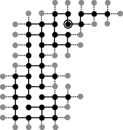
Figure 1: An open cluster (black solid dots) containing the origin (a black dot in a circle) as a result of percolation simulation on $\mathbb{L}^{2}$. Here the bond percolation probability $p$ was taken to be $0.478$; the solid segments represent open bonds. The open cluster can be seen as a finite outbreak of an epidemic with constant infectious periods and neighbour-to-neighbour infection intensity spread rate $\lambda_{ij}\approx 0.65$ (since $0.478=1-e^{-0.65}$). The dotted lines depict directions along which infection did not spread (from black to grey dots); thus, grey dots depict individuals which remain healthy and the dotted lines represent those bonds that must be closed given the knowledge of the cluster set.

Figure 1 depicts an open cluster obtained by simulation of percolation process on the integer lattice $\mathbb{Z}^{2}$ for $p=0.478$. This connected component containing the origin can be seen as a final (and finite) outbreak of an SIR epidemic process of the kind discussed above. The origin (or, indeed, any other vertex of the open cluster) may be considered to be the site where the initially inoculated individual has been placed. Clearly, the realised bond structure is not the only possible way which results in the site configuration from Figure 1. However, the distribution of this site configuration as an extinct SIR epidemic coincides with that of the corresponding unoriented bond percolation process.

III Parameter estimation

III.1 Scenario $\mathcal{S}1$

Let $\Pi$ be a (proper or improper) subgraph of $\mathbb{L}^{d}$ which contains the origin and let $\mathcal{C}$ be an open cluster of a percolation process on $\Pi$ containing the origin. The set of nodes $\mathcal{C}$ represents a snapshot of an extinct outbreak of our spatial SIR epidemic evolved on $\Pi\subseteq\mathbb{L}^{2}$.

Let us introduce some additional notions. Let $G=(V,E)$ be a locally finite graph and let $G^{\prime}=(V^{\prime},E^{\prime})$ be a subgraph of $G$ (that is $V^{\prime}\subseteq V$ and $E^{\prime}\subseteq E$). By the saturation of the graph $G^{\prime}$ with respect to $G$ we understand the graph $\tilde{G}=(\tilde{V},\tilde{E})$ such that

$$\tilde{V}=V^{\prime}\text{ and }\tilde{E}=\{(x,y)\,|\,x,y\in V^{\prime}\,\&\,(x,y)\in E\}.$$

We denote the saturation of $G^{\prime}$ with respect to $G$ by $\mathop{\rm Satur}\nolimits_{G}G^{\prime}$ or, in cases when it is clear from the context with respect to what graph the saturation takes place, by $\mathop{\rm Satur}\nolimits G^{\prime}$. A graph $G^{\prime}$ whose saturation coincides with itself is called a fully saturated graph. For example, the fully saturated graph (with respect to $\mathbb{L}^{2}$) is obtained from the graph depicted in Figure 1 by connecting all pairs of neighbouring black sites (according to the 4-neighbourhood relationship). Note that the operation of saturation may also be applied solely to a subset of vertices of the original graph, since it does not make use of the edges of the subgraph-operand.

To distinguish between the boundary points of a graph and their neighbours, which are not in the graph, we introduce the notions of the surface and the frontier of the graph (again, with respect to another graph). Let us denote by $\partial G$ the surface of $G$ in $\Pi$, $G\subseteq\Pi$, that is to say the set

$$\partial G:=\{x\in G:\,\exists y\in\Pi\backslash G\text{ s.t.\ }x\text{ and }y\text{ are neighbours in }\Pi\},$$

and by $\Gamma_{G}$ the frontier of $G$ in $\Pi$, i.e. the set $\partial(\Pi\backslash G)$.

In order to identify the likelihood function we introduce the set $\mathcal{G}(\mathcal{C})$ of all connected subgraphs of $\Pi$ with $\mathcal{C}$ as a vertex set. Note that the set $\mathcal{G}(\mathcal{C})$ is necessarily nonempty. For each $G\in\mathcal{G}(\mathcal{C})$ the number of edges between the vertices of the graph $G$ and the elements of its frontier $\Gamma_{G}$ is constant—we denote it by $w_{\mathcal{C}}$. Finally, we denote the total number of edges in $G$ by $e(G)$.

The probability that $\mathcal{C}$ represents the set of ever-infected sites and that the edges of $G$ correspond to those routes along which the infection travelled is

$$\mathbb{P}_{p}(G)=p^{e(G)}(1-p)^{e(\mathop{\rm Satur}\nolimits{\mathcal{C}})-e(G)+w_{\mathcal{C}}},$$

and the likelihood function associated with the observed set $\mathcal{C}$ of ever-infected sites is given by

$$\mathcal{L}(p)=\mathbb{P}_{p}(\mathcal{C})=\sum\limits_{G\in\mathcal{G}(\mathcal{C})}\mathbb{P}_{p}(G).$$

Hence, under assumption of a uniform prior for $p$, its posterior distribution $\pi(p\,|\,\mathcal{C})$ is a mixture of beta distributions:

$$\pi(p\,|\,\mathcal{C})\propto\sum\limits_{k}r(k)\thinspace\text{Beta}\left(k+1,e(\mathop{\rm Satur}\nolimits{\mathcal{C}})-k+w_{\mathcal{C}}+1\right),$$

where

$$r(k):=\#\{G\in\mathcal{G}(\mathcal{C})\,|\,e(G)=k\}.$$

It is not feasible to calculate $\pi(p\,|\,\mathcal{C})$ in the above form, since it is hard to enumerate all corresponding graphs and, thus, to calculate efficiently the coefficients $r(k)$. We describe therefore an McMC algorithm that allows one to sample from the distribution $\pi(p\,|\,\mathcal{C})$ under the uniform prior on $p$, that is, effectively, to estimate the likelihood function of $p$.

Our Markov chain explores the joint space $(0,1)\times\mathcal{G}(\mathcal{C})$ of possible values for $p$ and graphs from $\mathcal{G}(\mathcal{C})$. The stationary distribution of the chain is the joint posterior distribution of $p$ and $G\in\mathcal{G}(\mathcal{C})$. The description of the chain is given in Algorithm 1 (Appendix A.1). This Markov chain explores the set of all connected graphs $\mathcal{G}(\mathcal{C})$ by simply deleting or adding an edge from the current graph preserving the connectivity of the given site configuration $\mathcal{C}$.

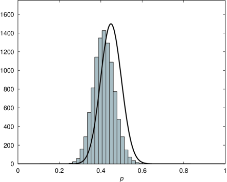
Figure 2: The solid line corresponds to the likelihood function evaluated for the complete information (both the sites and edges are known) on the cluster $\mathcal{C}$ from Figure 1. The histogram is based on a large sample drawn from the McMC applied to the site configuration $\mathcal{C}$ (nodes only).

We apply Algorithm 1 to the site configuration $\mathcal{C}$ from Figure 1 (black dots only). Figure 2 depicts the likelihood function of the model parameter for the complete observations (i.e. nodes and edges of the cluster) and a histogram of the sample obtained from the posterior distribution $\pi(p\,|\,\mathcal{C})$ when the prior distribution is uniform on the interval $(0,1)$.

Mixing properties of Markov chains described by Algorithm 1 are briefly discussed in Appendix B.

III.2 Scenario $\mathcal{S}2$

Under this scenario only the size $n$ of the outbreak of our SIR epidemic evolving on $\Pi=\mathbb{L}^{d}$ is given.

Let $\mathcal{G}_{n}$ be the set of all possible connected graphs on $n$ vertices including the origin. These graphs represent the outbreaks of the size $n$ and we distinguish all isomorphic graphs which have different locations or orientations.

We denote the number of edges of $\Pi$ between the vertices of the graph $G\in\mathcal{G}_{n}$ and the vertices of its frontier $\Gamma_{G}$ by $w(G)$.

Given the epidemic size $n$, the inference on $p$ involves evaluation of the likelihood function $\mathcal{L}_{n}(p):=\mathbb{P}_{p}(|\mathcal{C}|=n)$ which can be represented as follows:

$$\mathcal{L}_{n}(p)=\sum\limits_{G\in\mathcal{G}_{n}}\mathbb{P}_{p}(G).$$

As previously, under assumption of a uniform prior for $p$ its posterior distribution $\pi(p\,|\,|\mathcal{C}|=n)$ is a mixture of beta distributions:

$$\pi(p\,|\,|\mathcal{C}|=n)\propto\sum\limits_{s,k,l}q(s,k,l)\thinspace\text{Beta}\left(k+1,s-k+l+1\right),$$ (1)

where

$$q(s,k,l):=\#\{G\in\mathcal{G}_{n}\,|\,e(\mathop{\rm Satur}\nolimits{G})=s,e(G)=k,w(G)=l\}.$$

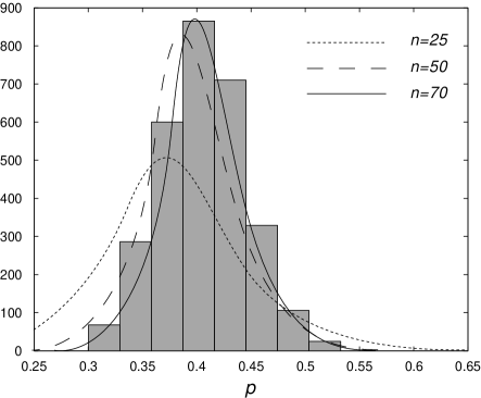
Figure 3: Likelihood functions $\mathcal{L}_{n}(p)$ ($n=25,50,70$) obtained using the McMC from Algorithm 2 and McMC sample histogram of $\mathcal{L}_{n}(p)$ for $n=70$.

This, again, represents a hard enumeration problem. However, inference on $p$ can be made using the McMC technique. Algorithm 2 (Appendix A.1) contains a description of a Markov chain which serves the purpose of sampling from the posterior distribution $\pi(p\,|\,|\mathcal{C}|=n)$, given the prior distribution of $p$ is uniform on [0,1]. The chain explores the joint space $(0,1)\times\mathcal{G}_{n}$ of possible values for the percolation parameter $p$ and all possible connected graphs on $n$ nodes, by deleting a vertex from a graph and adding a vertex from its frontier.

Figure 3 depicts plots of the likelihood function $\mathcal{L}_{n}$ when $n=25,\,50,\,70$ and a histogram of a sample drawn from $\pi(p\,|\,|\mathcal{C}|=70)$. The graphs of the likelihoods were obtained by smoothing the histograms of corresponding samples generated by the McMC presented in Algorithm 2. Note that, as might reasonably be expected, the values of $p$ maximising the likelihood increase with $n$.

Mixing properties of Markov chains described by Algorithm 2 are briefly discussed in Appendix B. Two video examples of dynamic graph updates illustrating Algorithms 1 and 2 can be found at the WEB address Bejan (2009).

III.3 Convergence analytical results for $\mathcal{S}2$

Percolation exhibits a phenomenon of criticality, this being central the percolation theory: as $p$ increases, the sizes of clusters (connected components) also increase, and there is a critical value of $p_{c}$ at which there appears a cluster which dominates the rest of the pattern. If $p<p_{c}$, then with probability one all open clusters are finite, but when $p>p_{c}$ there is a single infinite open cluster almost surely Grimmet (1999). Note, that the critical percolation parameter $p_{c}$ depends on the dimension $d$ of the lattice. Bond percolation on the square lattice seems to be most studied to date of all percolation processes. The critical probability $p_{c}$ in the case of a square lattice is $\frac{1}{2}$. What follows, however, holds for any lattice $\mathbb{Z}^{d}$, $d\geq 3$.

III.3.1 Asymptotic behaviour of the maximum likelihood estimates of $p$

Denote by $\mathcal{C}(x)$ the open cluster (connected component) which contains the vertex $x$. Let us write $\chi(p)=\mathbb{E}_{p}|\mathcal{C}|$ for the mean number of vertices in the open cluster at the origin. Using the translation invariance of the process on $\mathbb{Z}^{d}$, we have $\chi(p)=\mathbb{E}_{p}|\mathcal{C}(x)|$ for all vertices $x$. Percolation theory tells us that if $p<p_{c}$, then $\chi(p)<\infty$. When $p>p_{c}$, then $\chi(p)=\infty$ and the function $\chi$ is not of a much interest in this case. Instead, one studies the function $\chi^{f}(p)=\mathbb{E}_{p}[|\mathcal{C}|:|\mathcal{C}|<\infty]$. The function $\chi(p)$ ($\chi^{f}(p)$) monotonically increases to infinity as $p\uparrow p_{c}$ ($p\downarrow p_{c}$). It is known Grimmet (1999) that there is no infinite open cluster when $p=p_{c}$ for percolation on the square lattice $\mathbb{Z}^{2}$ and on the lattice $\mathbb{Z}^{d}$, where $d\geq 19$; this is also believed to be true for all other values of $d$. How likely it is to observe an open cluster of size $n$ when $n$ is very large? What value of $p$ should one suggest if one happened to observe a large epidemic of size $n$?

Intuitively, it is unlikely that very large but finite epidemics may be obtained for values of $p$ significantly different from $p_{c}$ (if $p\ll p_{c}$, then it is unlikely that the epidemic will attain a very large size; if $p\gg p_{c}$, then it is equally unlikely that, having attained a sufficiently large size $n$, the epidemic will have burned out). Intuition suggests therefore that the likelihood function for $p$, given that the size $n$ of the connected component containing the origin is growing, should be increasingly concentrated around $p_{c}$.

Let $\mathcal{L}_{n}(p)=\mathbb{P}_{p}(|\mathcal{C}|=n)$ be the probability that an open cluster $\mathcal{C}$ from a percolation process with the edge density $p$ is of size $n$. (Equivalently, assume that we observe an SIR spread of infection via nearest-neighbour interactions on $\mathbb{Z}^{d}$ and that the final size of its outbreak is $n$; when $n$ is fixed the function $\mathcal{L}_{n}(p)$ can be regarded as the likelihood function for the percolation probability parameter $p$.)

Let $\hat{p}_{n}$ be the maximum likelihood estimate for $p$ derived from $\mathcal{L}_{n}(p)$. For any $p$ define also $L_{n}(p)=\mathcal{L}_{n}(p)/\mathcal{L}_{n}(p_{c})$.

Theorem III.1

The sequence of maximum likelihood estimates $\hat{p}_{n}$ for $p$ converges to the critical probability $p_{c}$.

The proof of this theorem is based on the following lemma, together with a generally accepted regularity condition.

Lemma III.2

For any $p\in(0,1)$ different from $p_{c}$ the following holds:

$$\liminf\limits_{n\to\infty}L_{n}(p)=0.$$

Moreover, this convergence is uniform for any closed interval which does not contain $p_{c}$.

The proof of the lemma and the theorem can be found in Appendix A.2.

As mentioned above, it is reasonable to expect the sequence of the maximum likelihood estimates $\hat{p}_{n}$ to be monotonic (see Figure 3). This observation gives rise to the following conjecture.

Conjecture III.3

The sequence of $\{\hat{p}_{n}\}$ converges to $p_{c}$ monotonically from the left.

Furthermore, we formulate the corresponding companion conjecture for the sequence of posterior distribution, using the notion of a delta sequence Arfken (1985).

Conjecture III.4

Provided $p\in\text{supp}\thinspace\pi(\cdot)$ the functional sequence $\{\pi(p\,|\,n)\}_{n=1}^{\infty}$ is a delta sequence which generates the delta function $\delta(p-p_{c})$.

Thus, we believe that the limiting posterior distribution of the percolation parameter is a one-point mass distribution at $p=p_{c}$, or the Dirac delta function $\delta(p-p_{c})$.

III.3.2 Combinatorial characterisation of large percolation clusters on $\mathbb{L}^{d}$

The theoretical results obtained and conjectured previously for inference under scenario $\mathcal{S}2$ can be used to derive their combinatorial analogues regarding the relative number of realisations of the process with the cluster size $n$. Under scenario $\mathcal{S}2$ the posterior distribution $\pi(p\,|\,|\mathcal{C}|=n)$ can be seen as a mixture of beta distributions, as in (1). As in Section III.2, let $q(s,k,l)$ be the number of all possible graphs $G$ which may correspond to an open cluster $\mathcal{C}$ (the vertex set of $G$ and $\mathcal{C}$ coincide), and such that $k$ is the number of edges in $G$, $s$ is the number of edges in the saturation of $G$, and $l$ is the number of edges of $\Pi$ between the surface and the frontier of $G$. Conjecture III.4 would suggest that the number $q(s,k,l)$ of graphs $G$ corresponding to open clusters $\mathcal{C}$ which could emerge as a result of the percolation process with parameter $p_{c}$ and for which it holds that

$$\frac{k+1}{s+l+2}\approx p_{c},$$ (2)

is far greater than the number of all other graphs. This is so, since the sequence of beta distributions $\text{Beta}(\alpha_{n},\beta_{n})$ is a delta sequence generating the delta function at $p_{c}$ if and only if $\alpha_{n}/(\alpha_{n}+\beta_{n})\to p_{c}$.

Thus, in percolation processes on $\mathbb{L}^{d}$ the number of finite graphs corresponding to open clusters of size $n$ (where $n$ is large) that satisfy the condition

$$\frac{e(G)+1}{e(\mathop{\rm Satur}\nolimits{G})+w(G)+2}\approx p_{c}$$ (3)

largely exceeds the number of all other connected components on $n$ nodes. In other words, a typical graph corresponding to an open cluster of a large size in percolation process on $\mathbb{L}^{d}$ is a connected subgraph of $\mathbb{L}^{d}$ characterised by (3). In particular, when $d=2$:

$$e(G)-w(G)\approx e(\mathop{\rm Satur}\nolimits{G})-e(G);$$ (4)

that is the number of open edges in $G$ is approximately equal to the total number of closed edges and edges between $G$ and its frontier.

III.3.3 Large percolation clusters as rare events

When $n$ is large, the appearance of finite open clusters of size $n$ is highly unlikely: the distribution of the cluster size (hypothetically) decays as $n^{-1-1/\delta}$, $\delta>0$, when $p=p_{c}$, and the decay is exponential (sub-exponential) when $p<p_{c}$ ($p>p_{c}$). Large finite percolation clusters can therefore be viewed as rare events. Since the state space of the McMC proposed for inference on the percolation parameter $p$ under scenario $\mathcal{S}2$ and described in Algorithm 2 involves the set of all open clusters on $n$ nodes, this algorithm can be readily used in order to obtain realisations of these rare events.

IV Bayesian optimal designs

IV.1 Utility based optimal designs

IV.1.1 General description

The experimental design problem can be conveniently approached within the Bayesian framework Chaloner and Verdinelli (1995). Suppose we study a stochastic process for which we formulate a model $M$, characterised by a model parameter $\theta$. The model $M$ specifies a sampling density $f_{d}(y\,|\,\theta)$ for the experimental outcome $y$ obtained from observation of the process under experimental set-up $d$ given the value of the model parameter $\theta$. Our knowledge about $\theta$ is described by a prior distribution $\pi(\theta)$. Whenever the choice of set-up $d$ is under our control there arises the question of selecting the optimal $d$ under which one should observe the stochastic process. Such prescribed conditions are referred to as a design, and the optimal design is found under optimality criteria specifically tailored to the context and the purpose of the experiment.

By employing a utility function $u(d,y,\theta)$ one can specify the purpose of the experiment and measure the value of its outcome $y$ accordingly. The methodology of posing and solving utility-based optimal design problems within the Bayesian paradigm became somewhat standard Mueller (1999); Cook et al. (2008). The design has to be chosen before performing the experiment and one may choose to maximise the expectation of the utility function $u(d,y,\theta)$ with respect to $\theta$ and $y$ Mueller (1999):

$$d_{\text{max}}=\arg\max\limits_{d\in\mathcal{D}}U(d),$$ (5)

where

$$U(d)=\int\limits_{\Theta}\int\limits_{Y}u(d,y,\theta)f_{d}(y\,|\,\theta)\pi(\theta)\,\text{d}\theta\text{d}y.$$ (6)

Here $\mathcal{D}$ is the set of possible designs. The set of possible outcomes $y$ of the experiment is denoted by $Y$. The experiment is defined by a model $f_{d}(y\,|\,\theta)$, i.e. by the sampling density of $y$ conditional on $\theta$ for a given design $d$.

When the purpose of the experiment is to infer the model parameter, a sensible choice to measure the utility of the experiment under design $d$ might be one that represents the information gained on $\theta$ from the experiment. One of the standard choices is the Kullback–Leibler (KL) divergence $D_{\text{KL}}$ between the prior distribution of $\theta$, $\pi(\theta)$, and its posterior distribution $\pi(\theta\,|\,y,d)$ obtained following the experiment yielding data $y$:

$$D_{\text{KL}}\{\pi(\theta\,|\,y,d)\parallel\pi(\theta)\}=\int\limits_{\Theta}\log\frac{\pi(\theta\,|\,y,d)}{\pi(\theta)}\pi(\theta\,|\,y,d)\,\text{d}\theta,$$ (7)

where $\pi(\theta\,|\,y,d)\propto f_{d}(y\,|\,\theta)\pi(\theta)$.

Introduced by Kullback and Leibler Kullback and Leibler (1951) this information measure was justified by Lindley Lindley (1956) and Bernardo Bernardo (1979) and is related to the Shannon information measure.

The KL divergence is a random variable, being a function of the random outcome $y$. In order to find the the design $d_{\text{max}}$ that is optimal with respect to this choice of utility measure one should maximise the expected value of the KL divergence over the set of observables $Y$ as a function of the design variate $d$:

$$U_{\text{KL}}(d)=\mathbb{E}_{Y}[D_{\text{KL}}\{\pi(\theta\,|\,y,d)\parallel\pi(\theta)\}],$$ (8)

this being invariant under a reparametrisation of the model in terms of $\theta$.

When the experimental motivation consists in increasing one’s knowledge on the model parameter the expected KL divergence $U_{\text{KL}}(d)$ coincides with (6) taking $u(d,y,\theta)=\log\frac{\pi(\theta\,|\,y,d)}{\pi(\theta)}$. If, however, the purpose of the experiment is to inform someone who holds a different prior to our own and we wish to advise them on which design to use, using our own ‘superior’ knowledge of the system under study, then the expected KL divergence should be calculated in the form prescribed by (8) when the integration over the space of observables $Y$ is to be carried out using one’s superior knowledge. We refer to these contrasting experimental scenarios as progressive design and instructive design , respectively, and discuss them next in more detail.

IV.1.2 Progressive design

Under this scenario there is an experimenter $\mathscr{E}$ who holds prior beliefs regarding the parameter, $\theta$, in the form of a prior distribution $\pi(\theta)$ (perhaps obtained from earlier observation of the process) and whose goal is to design an optimal experiment in order to increase this knowledge. Using KL divergence as the measure of information gain, this experimenter should maximise the expected KL divergence (8):

$$U_{\text{KL}}(d) =\mathbb{E}_{Y}\mathbb{E}_{\Theta}\left.\left[\log\frac{\pi(\theta\,|\,y,d)}{\pi(\theta)}\,\right|\,y\right]$$

$$=\int\limits_{\Theta}\int\limits_{Y}\log\frac{\pi(\theta\,|\,y,d)}{\pi(\theta)}f_{d}(y,\theta)\,\text{d}\theta\text{d}y,$$

so that $U_{\text{KL}}(d)$ coincides with (6) where $u(d,y,\theta)=\log{\frac{\pi(\theta\,|\,y)}{\pi(\theta)}}$. Notice, however, that the expected information gain $U_{\text{KL}}(d)$ can be written as follows:

$$U_{\text{KL}}(d)= \int\limits_{Y}\int\limits_{\Theta}\log\pi(\theta\,|\,y,d)f_{d}(y\,|\,\theta)\pi(\theta)\,\text{d}\theta\text{d}y$$

$$-\int\limits_{\Theta}\log\pi(\theta)\pi(\theta)\,\text{d}\theta,$$

where the second term is the Shannon entropy of $\pi(\theta)$, which does not depend on $d$. Thus, in order to obtain the solution $d_{\text{max}}$ in this case, it suffices to maximise the first term only.

IV.1.3 Instructive design

In contrast to the progressive design scenario, in the instructive case there is an experimenter $\mathscr{E}$, holding a prior $\pi(\theta)$, and a better (or differently) informed trainer (or instructor) $\mathscr{T}$ whose knowledge about the model parameter is summarised in a distribution $\pi^{*}(\theta)$. (Of particular interest is a special case where the instructor knows the true value of $\theta$.) The aim here is to maximise the change in experimenter’s belief from $\pi(\theta)$ to $\pi(\theta\,|\,y)$ by designing an experiment using the superior knowledge $\pi^{*}(\theta)$.

This latter optimisation problem can be formulated as follows:

$$d^{*}_{\text{max}} =\arg\max\limits_{d\in\mathcal{D}}U^{*}_{\text{KL}}(d),$$ (9)

$$U^{*}_{\text{KL}}(d) =\int\limits_{Y}D_{\text{KL}}\{\pi(\theta\,|\,y,d)\parallel\pi(\theta)\}f^{*}(y)\,\text{d}y,$$ (10)

where, as before, $\pi(\theta\,|\,y)$ is derived as in (7), and $f^{*}(y)$ is the instructor’s prior predictive distribution for $y$:

$$f^{*}(y)=\int\limits_{\Theta}f_{d}(y\,|\,\theta)\pi^{*}(\theta)\,\text{d}\theta.$$

In particular, if the instructor $\mathscr{T}$ knows the exact value of $\theta$, $\theta^{*}$, and hence $\pi^{*}(\theta)$ is the Dirac function $\delta(\theta-\theta^{*})$, then $f^{*}(y)=f_{d}(y\,|\,\theta^{*})$, so that

$$U^{*}_{\text{KL}}(d)=\int\limits_{\mathcal{Y}}D_{\text{KL}}\{\pi(\theta\,|\,y,d)\parallel\pi(\theta)\}f_{d}(y\,|\,\theta^{*})\,\text{d}y.$$ (11)

Note that the ‘instructive’ expected utility $U^{*}_{\text{KL}}$ is generally not symmetric with respect to the exchange of $\pi(\theta)$ and $\pi^{*}(\theta)$: if the experimenter $\mathscr{E}$ and the instructor $\mathscr{T}$ change their roles, then the corresponding optimal instructive designs are different, unless their knowledge about $\theta$ is identical, that is $\pi(\theta)=\pi^{*}(\theta)$ almost everywhere.

IV.2 Simulation-based evaluation of the expected utility

Generally, the solution to the optimal design problems (5-6) and (9-10) cannot be obtained analytically. This is mainly due to the following three problems. First, the design space $\mathcal{D}$ can be complicated, with many design variables, some of them having a continuous range of values. Second, even if the design space has a simple structure, the utility function may not be simple to evaluate, so the expected utility $U(d)$ cannot be obtained explicitly. Finally, for incomplete observations of highly non-linear stochastic processes such as epidemic models, the likelihood is not usually available in a closed form, and this results in computationally intensive evaluations or sampling methods.

A review of analytical and approximate numerical solutions to Bayesian optimal design problems for traditional experimental design involving linear and non-linear models can be found in Verdinelli (1992); Chaloner and Verdinelli (1995).

Müller Mueller (1999) reviews simulation-based methods for optimal design problems where the expected utility $U(d)$ is evaluated by Monte-Carlo simulation. In its simplest form an estimate $\widehat{U}$ of $U$ for any given design $d$ in the progressive case is as follows:

$$\widehat{U}(d)=\frac{1}{M}\sum\limits_{i=1}^{M}u(d,\theta_{i},y_{i}),$$ (12)

where $\{(\theta_{i},y_{i}),i=1,\ldots,M\}$ is a Monte-Carlo sample generated values:

$$\theta_{i}\sim\pi(\theta),\thickspace y_{i}\sim p_{d}(y\,|\,\theta).$$ (13)

The expected utility $U$ may, in particular, be based on the KL divergence.

Analogously, the expected utility $U^{*}_{\text{KL}}$ under the instructive scenario, when the instructor knows the true value of the model parameter, $\theta^{*}$, can be evaluated using the following scheme:

$$\widehat{U}^{*}_{\text{KL}}(d)=\frac{1}{M}\sum\limits_{i=1}^{M}\widehat{KL}(y^{*}_{i},d),$$ (14)

where $y^{*}_{i}\sim f(y\,|\,\theta^{*},d)$, $i=1,\ldots,M$, and $\widehat{KL}(y_{i},d)$ is an estimate of the KL divergence $D_{\text{KL}}\{\pi(\theta\,|\,y^{*},d)\parallel\pi(\theta)\}$ that can be obtained via numerical integration of $\log\frac{\pi(\theta\,|\,y,d)}{\pi(\theta)}$ with respect to the posterior $\pi(\theta\,|\,y,d)$. The former function, in turn, may need to be evaluated through simulation methods—perhaps using an McMC scheme.

Evaluation of a continuous expected utility surface $U(d)$ by (12) or (14) can be achieved by computing its values on a discretised grid of points and further smoothing of the obtained set of values in order to approximate the expected utility landscape. This, however, may be problematic when $d\in\mathcal{D}$ is a multidimensional design parameter. An alternative method is provided by the augmented probability simulation approach which is studied in Clyde et al. (1995); Bielza et al. (1999), and reviewed in Mueller (1999).

The augmented probability simulation approach assumes that $u(d,\theta,y)$ is a non-negative bounded function. (This condition, although not always automatically satisfied, can be easily achieved by correspondingly modifying the utility function.) An artificial density, proportional to $u(d,\theta,y)f_{d}(y\,|\,\theta)\pi(\theta)$ can then be defined for $(d,\theta,y)$ jointly Mueller (1999):

$$h(d,\theta,y)\propto u(d,\theta,y)f_{d}(y\,|\,\theta)\pi(\theta),$$ (15)

so that its marginal in $d$ is proportional to the expected utility $U(d)$. Sampling from $h(\cdot,\cdot,\cdot)$ can be used to obtain a sample from its marginal using the Metropolis–Hastings McMC scheme described in Mueller (1999).

When using the augmented probability modelling approach one approximates the optimal design by an empirical mode of the marginal density of $d$ under the artificial distribution $h$, that is by the mode of histogram formed from the first components of the set of samples obtained. Notice that the evaluation of $u(d,\theta,y)$ at each sampling step may in general itself involve an McMC sampling from the posterior $\pi(\theta\,|\,y,d)$, so that the approach is potentially very expensive computationally.

IV.3 Inner-outer plots

We now apply the utility-based Bayesian approach introduced above in order to design optimal experiments for our SIR epidemic model with incomplete observations of the kind described by scenario $\mathcal{S}1$. We do so by identifying a (finite) class of designs (node configurations) which we call inner-outer plots. These are plots of bounded size which are obtained by removing some nodes from the underlying grid. We refer to this process as sparsification of the grid.

A typical example of an inner-outer plot in $\mathbb{Z}^{2}$ is given in Figure 4. The inner-outer plot depicted consists of two parts—inner and outer regions (hence the name of the design). Some sites are removed from the outer region of the plot in a regular manner, while all sites of the inner region are preserved. Our motivation in considering sparsified grids is to show that intuitively obvious designs, such as completely dense grids, can be improved. The justification of the grid sparsification is that it impedes the ability of the epidemic to spread, which makes possible better inference when $p$ is large, while the more dense inner part of the design works better when $p$ is small. A formal description of inner-outer plots follows next.

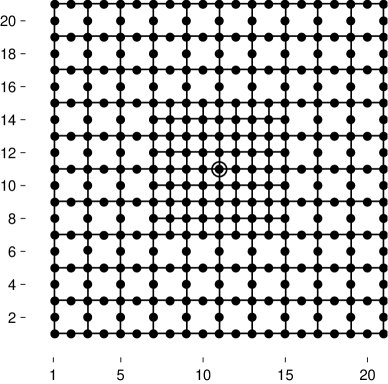
Figure 4: An example of an inner-outer $(m,r)$-plot (nodes only) in $\mathbb{Z}^{2}$. In this inner-outer plot $m=9$ and $r=3$. The plot is bounded by an $N\times N$ square, where $N=21$ can be calculated using (18). Depicted is the saturation of an $(9,3)$-plot with respect to $\mathbb{L}^{2}$.

Let us assume that $m$ is an odd positive integer and $r\in\mathbb{N}\cup\{0\}$. An inner-outer $(m,r)$-plot $\Pi^{(d)}_{0}(m,r)$ in $\mathbb{Z}^{d}$ with centre at the origin is a $d$-dimensional box $B_{N}^{(d)}$ with side-length $N=m+4r$ and some vertices removed as follows:

$$\Pi_{0}(m,r):=\begin{cases}B_{N}^{(d)},&r=0\\ B_{N}^{(d)}\setminus C_{N}^{(d)}(m,r),&r>0,\end{cases}$$ (16)

where $C_{N}^{(d)}(m,r)$ is the set

$$\{ x\in B_{N}^{(d)}:\,\parallel x\parallel_{\infty}=m+2j+1,j=0,\ldots,r-1\,\&\,$$

$$\&\parallel x\parallel_{1}\equiv 0\bmod 2\}.$$

Here $\parallel x\parallel_{1}=\sum\limits_{i=1}^{d}|x_{i}|$ and $\parallel x\parallel_{\infty}=\max(|x_{1}|,\ldots,|x_{d}|)$ for any $x=(x_{1},\ldots,x_{d})\in\mathbb{Z}^{2}$ and the box $B_{N}^{(d)}$ is defined as follows :

$$B_{N}^{(d)}: =[-(N-1)/2,(N-1)/2]^{d}$$

$$=\{x\in\mathbb{Z}^{d}:\,\parallel x\parallel_{\infty}\leq(N-1)/2\}.$$

We call any plot that can be obtained by translating the plot $\Pi^{(d)}_{0}(m,r)$ in $\mathbb{Z}^{d}$ an inner-outer $(m,r)$-plot, or simply an inner-outer plot, and denote it by $\Pi^{(d)}(m,r)$.

The total number of nodes contained in an $(m,r)$-plot can be calculated by subtracting the total number of the nodes removed from the outer plot (see (16)) as follows:

$$T =N(m,r)^{2}-4\sum\limits_{i=1}^{r}\left(\frac{m-1}{2}+2i-1\right)$$

$$=(m+3r)^{2}+r(3r+2),$$ (17)

where, as before,

$$N(m,r)=m+4r.$$ (18)

The inner-outer $(m,r)$-plot depicted in Figure 4 is from $\mathbb{Z}^{2}$. The size of the inner plot is $m\times m$, where $m=9$, and there are $r=3$ ‘circles’ (with respect to the metric $\parallel\cdot\parallel_{\infty}$) in the outer plot from which every second node is removed. The size of the bounding box is $N\times N$, where $N=m+4r=21$. The total number of nodes $T$ that this node configuration contains can be calculated using (17) and is equal to $357$.

IV.4 Inference for SIR epidemics on inner-outer plots

We consider an SIR epidemic with constant infectious times which arises at the central site of an inner-outer plot $\Pi=\Pi^{(d)}(m,r)$ from $\mathbb{Z}^{d}$ and evolves on that plot according to the nearest-neighbour interaction rule, that is using edges from $\mathbb{L}^{d}$ with endpoints from $\Pi$, subject to being restricted by the plot boundary. We consider this model in the context of scenario $\mathcal{S}1$, that is when the only information available about the outcome of the epidemic is its site configuration $\mathcal{C}$. As before, this model is equivalent to that of percolation on $\Pi^{(d)}(m,r)$.

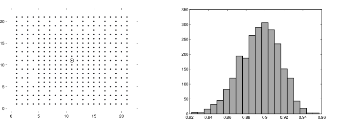
Figure 5: Left: site configuration obtained on the inner-outer $(13,2)$-plot with $p=0.9$. Right: McMC histogram of an McMC sample for $p$ assuming a uniform prior for this parameter.

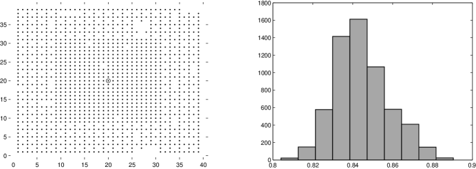
Figure 6: Left: site configuration obtained on the inner-outer $(23,4)$-plot with $p=0.86$. Right: histogram of an McMC sample for $p$ assuming a uniform prior for this parameter.

We note that Algorithm 1 and Algorithm 2 can be readily used for making inference on the percolation probability parameter $p$ given the sites of an open cluster $\mathcal{C}$, or merely its size in the case of Algorithm 2, generated from a percolation process on any locally finite graph .

Figure 6 shows the plot of a simulated open percolation cluster $\mathcal{C}$ obtained on the inner-outer plot $\Pi^{(2)}(13,2)$ with $p=0.9$ (left plot) and an estimate of the likelihood formed from a histogram estimate of the posterior density of $p$ obtained using the Markov chain described in Algorithm 1 with $\mathcal{C}$ as the input data, with a uniform prior density for $p$. Figure 5 shows similar plots for a realisation of the percolation process on $\Pi^{(2)}(23,4)$ with $p=0.86$.

IV.5 Optimal design problem and design space

We consider now an optimal design problem for the percolation process on node sets of limited size. We adopt the utility-based Bayesian approach formulated in Section IV.1. The choice of the design space $\mathcal{D}$ can be made in a number of ways, possibly reflecting such restrictions as limitations on the number of experimental units or the dimensions of the experimental plot. In the context of inner-outer plots the former restriction would mean that $T$ from (17) is bounded, whereas the latter condition is equivalent to bounding the quantity $N(m,r)$. A combination of these conditions or some other information can be also taken into account when identifying the design space. One advantage of grid-based plot designs is that they can greatly reduce the dimensionality of the design space compared with designs that allow units to be placed at arbitrary locations.

We assume now that $N$ is odd and fixed and that the design space has the form

$$\mathcal{D}=\{d\,|\,d=\Pi^{(2)}(m,r)\thickspace\&\thickspace m+4r=N\}$$

For example, if $N=19$ then, as can be derived easily from (18), the design space consists of the following designs:

$$\mathcal{D}=\{ \Pi^{(2)}(19,0),\,\Pi^{(2)}(15,1),\,\Pi^{(2)}(11,2),\,$$

$$\Pi^{(2)}(7,3),\,\Pi^{(2)}(3,4)\}.$$

The set of observables $Y$ is the set of all connected components on $d\in\mathcal{D}$ containing the central node.

V Practical implementation

Given a finite design space $\mathcal{D}$ it is fairly straightforward to solve the optimal design problem for the percolation model on inner-outer plots using the tools developed above. We now make some comments about solving the problem under each of the two design scenarios.

V.1 Progressive design: expected utility evaluation through augmented modelling

Since $\mathcal{D}$ is finite we choose to identify the design that maximises the expected utility function in the progressive case using augmented modelling as described in Section IV.2. Recall that this is based on an artificial distribution $h(d,p,y)\propto u(d,p,y)f_{d}(y\,|\,p)\pi(p)$ from which samples are generated using a Metropolis–Hastings sampler. The optimal design $d^{*}$ is identified then as a value of $d$ at which the marginal of $h$ is maximised.

V.2 Instructive design: Monte Carlo evaluation of the expected utility

We treat the ‘instructive’ case differently from that of the ‘progressive’ one because of the form of the expected utility under this scenario. Recall that in the ‘instructive’ case whenever the instructor knows the true value $p^{*}$ of the model parameter $p$ one can write the expected utility based on the Kullback–Leibler divergence as follows (compare with (11)):

$$U^{*}_{\text{KL}}(d)=\sum\limits_{y\in\mathcal{Y}}f_{d}(y\,|\,p^{*})\int\limits_{0}^{1}\log\frac{\pi(p\,|\,y,d)}{\pi(p)}\pi(p\,|\,y,d)\,\text{d}p,$$

where $f_{d}(y\,|\,p^{*})$ is the likelihood function evaluated at the true value of the model parameter $p^{*}$ given the open cluster $y$ at the centre of the inner-outer plot $d$.

It is clear that to evaluate the expected utility $U^{*}_{\text{KL}}(d)$ via standard Monte Carlo simulation, then a Markov chain has to be run to evaluate the posterior $\pi(p\,|\,y,d)$ each time we sample for a new observation (an open cluster) $y$ and also the potentially time-consuming integration has to be done with respect to the model parameter $p$. This integration can be implemented in the following way. Since we can sample from the posterior $\pi(p\,|\,y,d)$ via McMC (Algorithm 1) for any given open cluster $y$, we do so and then fit the beta distribution (or some other distribution) to the McMC sample obtained in order to perform integration numerically in a more efficient, albeit, approximate manner.

Thus, the expected utility evaluation scheme for inner-outer plots in the ‘instructive’ case and scenario $\mathcal{S}1$ can be described as follows.

For each inner-outer plot $d\in\mathcal{D}$ we do the following:

1. generate a random sample of $M$ independent connected clusters $\{y_{i}\}_{i=1}^{M}$ on $\Pi(m,r)$: $y_{i}\sim f(y\,|\,p^{*},d)$;

2. perform $M$ McMC’s in order to obtain $M$ independent samples for the posterior distribution $\pi(p\,|\,y,d)$;

3. fit a Beta distribution to each of the samples obtained; refer to the fitted distributions as $\pi(p\,|\,y_{i},d)$;

4. evaluate numerically the integrals

   $$I_{i}:=\int_{0}^{1}\log\frac{\pi(p\,|\,y_{i},d)}{\pi(p)}\pi(p\,|\,y_{i},d)\,\text{d}p;$$

5. estimate the expected utility: $\bar{U}_{M}=\frac{1}{M}\sum\limits_{i=1}^{M}I_{i}.$

It is natural to ask how well the true posteriors can be fitted by a Beta distribution (step (iii) of the above scheme). Experience suggests that such a fit never affects the outcome of the analysis on the qualitative level unless the prior distribution has more than one local mode or its support is smaller than the entire interval $(0,1)$. Recall that the purpose of this step is to make evaluation of the integrals $I_{i}$ easier and faster, and hence the family of Beta distributions is only one possible choice. For instance, if the prior distribution $\pi(p)$ is uniform on $(0,1)$, then the integrals $I_{i}$ represent the entropies of the fitted distributions. In the case when the fitting is done by beta distributions, each of these integrals can be quickly calculated using the following analytical formula for the entropy of the beta distribution $\text{Beta}(\alpha,\beta)$:

$${\rm Ent}\{\text{Beta}(\alpha,\beta)\}= \log B(\alpha,\beta)+(\alpha+\beta-2)\psi(\alpha+\beta)$$

$$-(\alpha-1)\psi(\alpha)-(\beta-1)\psi(\beta),$$

where $\psi$ is the digamma function, $\psi(z)=\Gamma^{\prime}(x)/\Gamma(z)$. Other choices of prior distribution may suggest alternative and more appropriate fitting distributions to facilitate the calculation of the integrals $I_{i}$, $i=1,\ldots,M$.

V.3 Example

In our example we consider all inner-outer plots in $\mathbb{L}^{2}$ whose sizes do not exceed $N=11$. There are only three such plots: $\Pi^{(2)}(3,2)$, $\Pi^{(2)}(7,1)$, and $\Pi^{(2)}(11,0)$. For ease of reference we mark them A, B, and C respectively (as depicted in Figure 7). Thus, the design space $\mathcal{D}=\{\text{A},\text{B},\text{C}\}$ consists of three designs, among which A is the most sparsified plot whereas no nodes are removed from C at all.

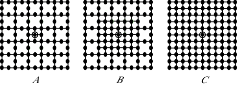
Figure 7: Inner-outer design plots $A$, $B$, and $C$ form the design space $\mathcal{D}=\{A,B,C\}$.

Figure 8 represents graphically the results of the comparison of designs from $\mathcal{D}$ under both ‘progressive’ and ‘instructive’ scenarios when the prior distribution $\pi(p)$ is uniform on the interval $(0,1)$. The left panel of the figure corresponds to the former scenario and depicts a histogram of a sample corresponding to the marginal of the artificial augmenting distribution $h(d,p,y)\propto u(d,p,y)f(y\,|\,p,d)\pi(p)$ in $d\in\mathcal{D}$. The right panel corresponds to the latter scenario and shows the Monte Carlo estimated values of the expected utilities and 95% credibility intervals for each of the three considered designs ($M=1500$, see (12) in Section IV.2) assuming that the instructor knows $p$ precisely so that $\pi^{*}(p)=\delta(p-0.9)$.

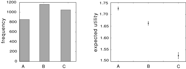
Figure 8: Left: sample histogram for the marginal of $h(d,p,y)$ in $d$, $d\in\{\text{A},\text{B},\text{C}\}$, under progressive design and $\pi(p)\sim\text{U}(0,1)$. Right: evaluated expected utility under instructive design with $\pi^{*}(p)\equiv\delta(p-0.9)$ and 95% credibility intervals ($M=1500$) for the plots A, B, and C, under instructive design.

The plots from Figure 8 indicate that the solutions to the optimal design problem under the two scenarios are different from each other. The ‘moderately sparsified’ plot B maximises the expected utility in the progressive case, that is in the case when the experiment is designed by a single experimenter. If, however, it is the instructor who knows the true value of the model parameter ($p=0.9$) and wishes to choose the best inner-outer plot from the set $\mathcal{D}$ for a more uninformed experimenter to use (instructive scenario), then the optimal plot is the ‘mostly sparsified’ inner-outer plot A. Notably, the ‘mostly dense’ plot C would be the worst choice in the instructive case, whereas it outperforms the ‘mostly sparsified’ plot A but is worse than the ‘moderately sparsified’ plot B in the progressive case. These results demonstrate the moderately counter-intuitive finding that the optimal design is not necessarily that with the maximal number of experimental units and that a ’less-is-more’ principle may be in operation. On another level, this finding may not be entirely unpredictable in the instructive case. The optimal design’s combination of a dense centre and sparsified outer region may help to increase the probability that the experimental epidemic succeeds in establishing itself but does not lead to saturation of the lattice before it dies out. This in turn may represent an outcome that yields much information on the unknown $p$.

VI Concluding comments

In this paper we have considered a number of question relating to the observation of percolation processes on finite lattices. We have demonstrated the value of McMC techniques for parameter estimation under different sampling regimes and shown how Bayesian experimental design techniques can be used to identify the optimal lattices on which to carry out experiments.

We introduced inner-outer plot designs by sparsifying the underlying grid. Allowing one to control excessive connectivity in outer regions of experimental plots, these designs help to separate different values of the model parameter $p$ when $p\gg p_{c}$, while giving the epidemic a chance to establish in inner regions when $p\ll p_{c}$. Inner-outer plots can be further generalised by considering more than two levels of grid sparsification, according to the principle used in our work: the farther the region is from the centre of the plot the more intensive sparsification it receives. To an extent, this process can be viewed as switching to similarly shaped lattices with percolation parameter taking its values from the set $\{p,p^{2},p^{3},\ldots\}$ in decreasing fashion.

Although we have worked largely within framework of percolation theory, the connection between percolation and spatio-temporal epidemic models with nearest-neighbour interactions mean that the results may have significant implications for and application to the study of epidemic systems.

Appendix A Algorithms and proofs

A.1 McMC algorithms for the scenarios $\mathcal{S}1$ and $\mathcal{S}2$

An McMC algorithm for making inference on the percolation probability $p$ under scenario $\mathcal{S}1$ is given in Algorithm 1. The proposed McMC is irreducible by construction: there is a positive probability for the chain to switch between any two connected graphs from $\mathcal{G}(\mathcal{C})$, since any two such graphs share a common vertex set and differ only by a finite number of edges.

Algorithm 1 Markov Chain Monte Carlo: scenario $\mathcal{S}1$

0:  an open cluster $\mathcal{C}$;

1:  take an initial value $p_{0}$ arbitrary from $(0,1)$;

2:  $t:=0$ $X_{t}:=(p_{t},\mathop{\rm Satur}\nolimits{\mathcal{C}})$;

3:  repeat

4:     Gibbs sampler steps:

5:     $p_{2t+1}\sim\text{Beta}\left(e(G_{2t})+1,e(\mathop{\rm Satur}\nolimits{\mathcal{C}})-e(G_{2t})+w_{\mathcal{C}}+1\right)$;

6:     $X_{2t+1}:=(p_{2t+1},G_{2t})$;

7:     Metropolis–Hastings sampler steps:

8:     choose an edge $e$ uniformly at random from $\mathop{\rm Satur}\nolimits{\mathcal{C}}$;

9:     if $e\in G_{2t}$ then

10:        $U\sim\text{Uniform}[0,1]$;

11:        if  $U\leq\min(1,\frac{1-p_{2t+1}}{p_{2t+1}}1{\text{\rm l}}_{\{G_{2t+1}\setminus\{e\}\text{ is connected}\}})$ then

12:           $X_{2t+2}:=(p_{2t+1},G_{2t+1}\setminus\{e\})$;

13:        else

14:           $X_{2t+2}:=(p_{2t+1},G_{2t+1})$;

15:     else

16:        $U\sim\text{Uniform}[0,1]$;

17:        if $U\leq\min(1,\frac{p_{2t+1}}{1-p_{2t+1}})$ then

18:           $X_{2t+2}:=(p_{2t+1},G_{2t+1}\cup\{e\})$;

19:        else

20:           $X_{2t+2}:=(p_{2t+1},G_{2t+1})$;

21:     $t:=t+2$;

22:  until we judge that the chain has converged and a sample of sufficient size is obtained

Algorithm 2 describes an McMC algorithm for making inference on $p$ under scenario $\mathcal{S}2$. This algorithm, similarly to Algorithm 1, is a combination of Gibbs and Metropolis–Hastings steps. The chain’s stationary distribution $f(p,G)$ specified a marginal density for $p$ which coincides with the posterior distribution $\pi(p\,|\,|\mathcal{C}|=n)$.

Algorithm 2 Markov Chain Monte Carlo: scenario $\mathcal{S}2$

0:  the value of $n$.

1:  take a value $p_{0}$ arbitrary from $(0,1)$ and a graph $G_{0}$ arbitrary from $\mathcal{G}_{n}$;

2:  $t:=0$ $X_{t}:=(p_{t},G_{t})$;

3:  repeat

4:     move_on:=1;

5:     Gibbs sampler steps:

6:     $p_{2t+1}\sim\text{Beta}\left(e(G_{2t})+1,e(\mathop{\rm Satur}\nolimits{G_{2t}})-e(G_{2t})+w(G_{2t})+1\right)$;

7:     $X_{2t+1}:=(p_{2}t+1,G_{2t})$;

8:     Metropolis–Hastings sampler steps:

9:     choose a vertex $u$ uniformly at random from $G_{2t+1}$ and choose a vertex $v$ uniformly at random from $\Gamma_{G_{2t+1}}$. Derive a graph $\tilde{G}$ from $G_{2t+1}$ by deleting all edges which adjoin $u$ (in $G_{2t+1}$) and adding the edges that connect $v$ with vertices of the graph $G_{2t+1}\setminus\{u\}$ in $\Pi$, each independently with probability $p_{2t+1}$ (conditioning on the event that at least one edge is added).

10:     if $\tilde{G}$ is disconnected then

11:        $X_{2t+2}:=(p_{2t+1},G_{2t+1})$; move_on:=0

12:     if move_on then

13:        $U\sim\text{Uniform}(0,1)$;

14:        $\tilde{d}(v):=\#\{e\,|\,e=(v,z)\thinspace\exists z\in G_{2t+1}\setminus\{u\}\}$;

15:        $\tilde{d}(u):=\#\{e\,|\,e=(u,z)\thinspace\exists z\in\tilde{G}\setminus\{v\}\}$;

16:        $\nu(u):=\#\{x\,|\,x\in\Gamma_{G_{2t+1}}\,\&\,(u,x)\in\Pi\}$;

17:        $\nu(v):=\#\{x\,|\,x\in\Gamma_{\tilde{G}}\,\&\,(v,x)\in\Pi\}$;

18:        $\kappa:=\tilde{d}(u)-\tilde{d}(v)+\nu(v)-\nu(u)$; $U\sim\text{Uniform}(0,1)$;

19:        if $U\leq\min\left(1,\frac{|\Gamma_{G_{2t+1}}|}{|\Gamma_{\tilde{G}}|}\frac{1-(1-p_{2t+1})^{\tilde{d}(v)}}{1-(1-p_{2t+1})^{\tilde{d}(u)}}(1-p_{2t+1})^{\kappa}\right)$ then

20:           $X_{2t+2}:=(p_{2t+1},\tilde{G})$;

21:        else

22:           $X_{2t+2}:=(p_{2t+1},G_{2t+1})$;

23:     $t:=t+2$;

24:  until we judge that the chain has converged and a sample of sufficient size is obtained

We give now explicit expressions for the proposal probabilities used in the Metropolis–Hastings steps within this algorithm. Assume that the current graph within the Metropolis–Hastings step is $G$ and a graph $\tilde{G}$ is proposed, the latter being obtained from the former by deleting a vertex $u$ with all edges adjoining it and inserting a vertex $v$, including each potential edge to $v$ independently with probability $p$, this probability having been drawn in the preceding Gibbs step. We assume that at least one such edge is inserted and denote the number of deleted and added edges by $d(u)$ and $d(v)$ respectively. Then,

$$q(G,\tilde{G})=\frac{1}{n}\frac{1}{|\Gamma_{G}|}\frac{p^{d(v)}(1-p)^{\tilde{d}(v)-d(v)}}{1-(1-p)^{\tilde{d}(v)}}1{\text{\rm l}}_{\{\tilde{G}\text{ is connected}\}},$$ (19)

and similarly,

$$q(\tilde{G},G)=\frac{1}{n}\frac{1}{|\Gamma_{\tilde{G}}|}\frac{p^{d(u)}(1-p)^{\tilde{d}(u)-d(u)}}{1-(1-p)^{\tilde{d}(u)}}1{\text{\rm l}}_{\{G\text{ is connected}\}}.$$ (20)

Clearly,

$$\mathbb{P}_{p}(G) \propto p^{d(u)}(1-p)^{\tilde{d}(v)}(1-p)^{\tilde{d}(u)-d(u)+\nu(u)}$$

$$\mathbb{P}_{p}(\tilde{G}) \propto p^{d(v)}(1-p)^{\tilde{d}(v)}(1-p)^{\tilde{d}(v)-d(v)+\nu(v)},$$

so that the acceptance probability at the Metropolis–Hastings step, $\alpha$, is as follows:

$$\alpha =\min\left(1,\frac{q(\tilde{G},G)}{q(G,\tilde{G})}\frac{\mathbb{P}_{p}(\tilde{G})}{\mathbb{P}_{p}(G)}\right)$$

$$=\min\left(1,\frac{|\Gamma_{G}|}{|\Gamma_{\tilde{G}}|}\frac{(1-p)^{\tilde{d}(u)+\nu(v)}}{(1-p)^{\tilde{d}(v)+\nu(u)}}\frac{1-(1-p)^{\tilde{d}(v)}}{1-(1-p)^{\tilde{d}(u)}}\right)$$

$$=\min,\left(1,\frac{|\Gamma_{G}|}{|\Gamma_{\tilde{G}}|}\frac{1-(1-p)^{\tilde{d}(v)}}{1-(1-p)^{\tilde{d}(u)}}(1-p)^{\kappa}\right),$$

where, as it was introduced in the description of Algorithm 2,

$$\kappa=\tilde{d}(u)-\tilde{d}(v)+\nu(v)-\nu(u).$$

We claim that the constructed chain is irreducible. In terms of graph theory this means that the chain can proceed from each connected graph on $n$ vertices, including the origin, to any other connected graph including the origin of the same size on the underlying lattice. We show the irreducibility of the proposed McMC by constructing a sequence of steps in which any graph of $\mathcal{G}_{n}$ is transformed to a so called line-skeleton graph on $n$ vertices. By such a graph we mean any tree (a graph with no cycles) containing the origin and having $n$ vertices so that only two of these vertices have degree one. Select one such line-skeleton and denote it by $S$.

Consider a graph $G$ from $\mathcal{G}_{n}$ and denote the length of the shortest open path from $x\in G$ to $S$ by $\delta(x,S)$ (chemical distance). Each vertex $x$ from $G$ receives a well defined finite weight $\delta(x,S)$, since the graph $G$ is connected and finite. By using the description of our Markov chain we can delete any vertex from our current graph for which $\delta(x,S)$ is maximal and add to this graph a vertex from the chosen line skeleton $S$ without making the graph disconnected or containing cycles until the maximum value of $d(x,S)$ is zero—in this case all vertices are forming the line skeleton. Since this procedure can be reversed it follows that $\mathcal{G}_{n}$ in the described Markov chain is indeed a communicating class, and hence the chain is irreducible.

A.2 Lemma and Theorem

Proof. (Lemma III.2) We consider the following two cases Grimmet (1999):

1. Subcritical case $p<p_{c}$. In this case the cluster size distribution $\mathcal{L}_{n}(p)$ decays exponentially, i.e.

   $$\exists\,\lambda(p)>0:\thickspace\mathcal{L}_{n}(p)\leq e^{-n\lambda(p)}\thickspace\forall n\geq 1.$$ (21)

   However, it is also known that at $p=p_{c}$ the cluster size distribution, while almost surely finite, nevertheless has an infinite mean. This implies that, for any $\lambda$ such that $0<\lambda<\lambda_{p}$, we have $\limsup\limits_{n\to\infty}e^{\lambda n}\mathcal{L}_{n}(p_{c})=\infty$, which when combined with (21), gives $\liminf\limits_{n\to\infty}L_{n}(p)=0$, as required. Uniformity of convergence on any closed interval contained within $(0,p_{c})$ follows since $\lambda$ above may be chosen so that $\lambda_{p}$ is uniformly bounded away from $\lambda$ for $p$ belonging to such an interval.

2. Supercritical case $p>p_{c}$. The argument here is essentially the same. In this case the decay is sub-exponential:

   $$\exists\,\eta(p)>0:\thickspace\thickspace\mathcal{L}_{n}(p)\leq e^{-\eta(p)n^{(d-1)/d}}\thickspace\forall n\geq 1.$$ (22)

   The infinite mean of the cluster size at $p=p_{c}$ also implies that for any $\eta$ such that $0<\eta<\eta_{p}$, we have $\limsup\limits_{n\to\infty}e^{\eta n^{(d-1)/d}}\mathcal{L}_{n}(p_{c})=\infty$, which, when combined with (22), again gives $\liminf_{n\to\infty}L_{n}(p)=0$, as required. Uniformity of convergence on any closed interval contained within $(p_{c},1)$ follows as before, and, when taken with the earlier result, gives the uniformity assertion of the lemma.

 

Proof. (Theorem III.1) We assume only that $\lim_{n\to\infty}L_{n}(p)$ exists. Then, by Lemma III.2 this limit is equal to zero for all $p\neq p_{c}$. (The existence of the limit would follow, for example, from the widely believed, but not rigorously proved, result that for $p=p_{c}$ the distribution of the size of the open cluster size containing the origin has a power-law tail—see Chapter 9 of Grimmet (1999).) Then the result of Lemma III.2 can be reformulated in $\varepsilon$-terms as follows: $\forall\varepsilon>0\thickspace\exists\,N(\varepsilon,\gamma)>0$, such that

$$\mathcal{L}_{n}(p)<\varepsilon\mathcal{L}_{n}(p_{c})\,\forall n>N(\varepsilon,\gamma)\,\forall p\in[\alpha,p_{c}-\gamma]\cup[p_{c}+\gamma,\beta),$$ (23)

for any $\alpha$ and $\beta$, such that

$$\Delta=[\alpha,p_{c}-\gamma]\cup[p_{c}+\gamma,\beta],\,\Delta\subset(0,1).$$

The quantity $\hat{p}_{n}$, being the maximum likelihood estimate for $p$, is the mode of $\mathcal{L}_{n}(p)$:

$$\hat{p}_{n}:=\text{arg}\max\limits_{p\in(0,1)}\mathcal{L}_{n}(p),$$

that is

$$\mathcal{L}_{n}(\hat{p}_{n})\geq\mathcal{L}_{n}(p)\thickspace\forall p\in(0,1).$$ (24)

Consider the sequence of mle’s $\{\hat{p}_{n}\}_{n=1}^{\infty}$. We now prove that this sequence converges to $p_{c}$. Suppose, conversely, this is not the case:

$$\exists\,\zeta\in(0,1)\thinspace\forall M>0\thinspace\exists\,n>M:\thinspace|\hat{p}_{n}-p_{c}|>\zeta.$$

Take $M(\zeta)=N(\zeta,\zeta/2)$, then $\exists\,n>M(\zeta):\thinspace|\hat{p}_{n}-p_{c}|>\zeta$, and, thus, $p_{c}\neq\hat{p}_{n}$. At the same time (when $\varepsilon=\zeta$) the following holds by (23):

$$\mathcal{L}_{n}(\hat{p}_{n})<\zeta\mathcal{L}_{n}(p_{c})<\mathcal{L}_{n}(p_{c}),$$

thereby contradicting (24). Hence, $\hat{p}_{n}\rightarrow p_{c}$, $n\rightarrow\infty$.   

Appendix B Mixing properties of chains from the proposed algorithms

Scenario $\mathcal{S}1$ and Algorithm 1. Figure 9 displays a trace plot of updates in $p$ for inference made for the site configurations from Figure 1 (Algorithm 1 was applied) and presented in Figure 2. The trace plot indicates that the mixing properties of the chain are rather satisfactory. The Matlab-based simulation used required 15 seconds on Intel(R) Core(TM)2 Duo CPU 2.26GHz to obtain a series of chain updates of the length $10^{4}$.

Experiments with larger configurations suggest that the burn-in time of the constructed chain may vary considerably with the size of the site configuration and its potential connectivity properties as well as on the choice of the initial graph $G_{0}$ (in our experiments we worked with fully saturated graphs and with connected components derived from those by random sparsification of edges). However, in practice, the chain described by Algorithm 1 typically converges rapidly: both the connected component updates and the percolation parameter updates can be efficiently realised, allowing one to generate a suitable sample from the posterior distribution $\pi(p\,|\,\mathcal{C})$ within practically useful timescales. Updates of the connected component, that is deletion and insertion of edges while preserving the connectedness of the underlying graph, can be further improved using dynamic graph algorithms Zaroliagis (2002).

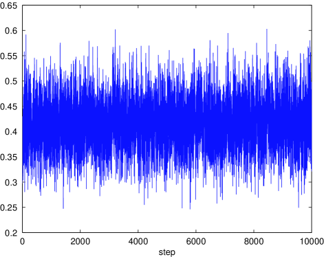
Figure 9: Trace plot for McMC sampling resulted in the histogram from Figure 2 for the cluster $\mathcal{C}$ in Figure 1.

Scenario $\mathcal{S}2$ and Algorithm 2. Figure 10 shows histograms of samples from the distribution $\pi(p\,|\,|\mathcal{C}|=n)$ obtained using the proposed McMC for the scenario $\mathcal{S}2$ for the cluster size values $p=10,\,35,\,50,\,70$ and corresponding trace plots.

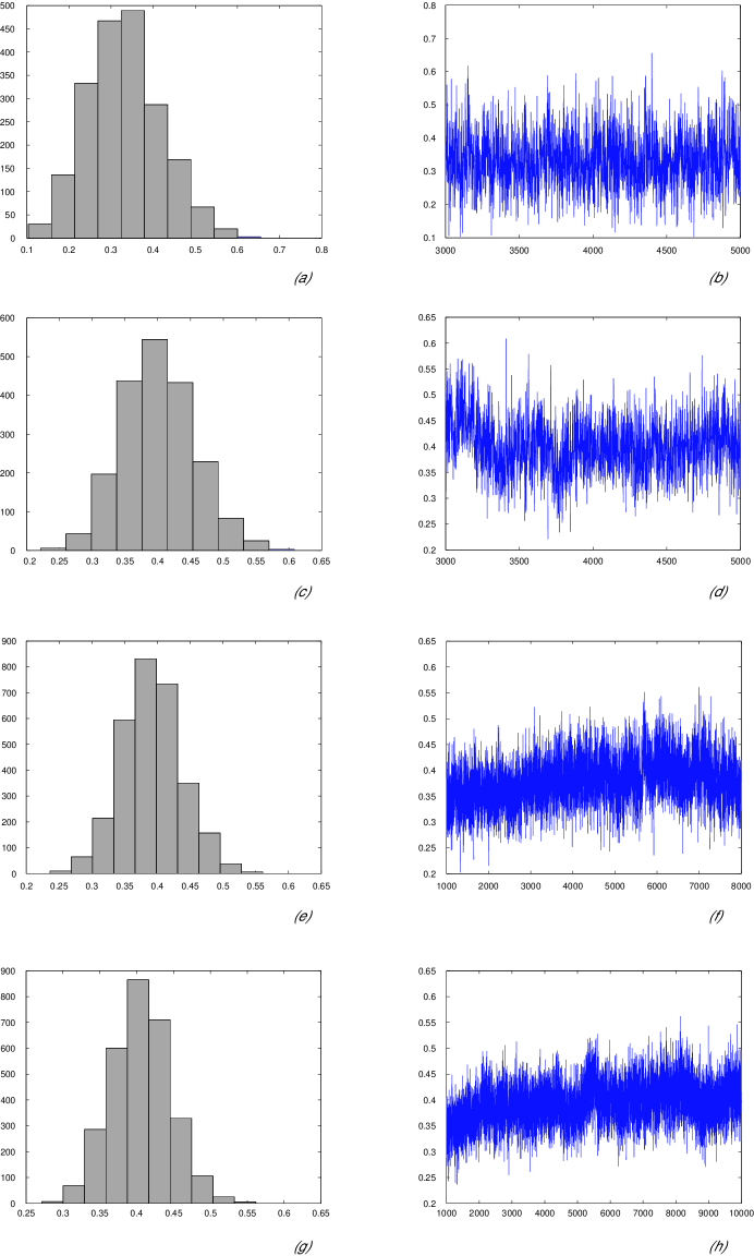
Figure 10: Inference on the percolation parameter using McMC described in Algorithm 2: histograms of obtained samples and trace plots for (a,b) $n=10$; (c,d) $n=35$; (e,f) $n=50$; (g,h) $n=70$.

References

- Gibson et al. (2006) G. J. Gibson, W. Otten, J. A. N. Filipe, A. Cook, G. Marion, and C. A. Gilligan, Stat. Comput. 16, 391 (2006).
- Chase (1998) A. R. Chase, Western connection. Turf and ornamentals 1, 1 (1998).
- Gibson et al. (2004) G. J. Gibson, A. Kleczkowski, and C. A. Gilligan, Proc. Nat. Acad. Sci. 101, 12120 (2004).
- Otten et al. (2004) W. Otten, D. J. Bailey, and C. A. Gilligan, New Phytol. 163, 125 (2004).
- Bailey and Gilligan (1997) D. J. Bailey and C. A. Gilligan, New Phytol. 136, 359 (1997).
- Bailey et al. (2000) D. J. Bailey, W. Otten, and C. Gilligan, New Phytol. 146, 535 (2000).
- Sahimi (1994) M. Sahimi, Applications of Percolation Theory (Taylor & Francis, 1994), ISBN 0-7484-0076-1.
- Frisch and Hammersley (1963) H. L. Frisch and J. M. Hammersley, J. Ind. Appl. Math. 11, 894 (1963).
- Zhang (1993) Y. Zhang, Ann. Probab. 21, 1755 (1993).
- Cox and Durrett (1988) J. T. Cox and R. Durrett, Stochastic Process Appl. 30, 171 (1988).
- Keeling et al. (2004) M. J. Keeling, S. P. Brooks, and C. A. Gilligan, Proc. Nat. Adac. Sci. 101, 9155 (2004).
- Gibson (1997) G. J. Gibson, Appl. Stat. 46, 215 (1997).
- Chaloner and Verdinelli (1995) K. Chaloner and I. Verdinelli, Stat. Sci. 10, 273 (1995).
- Mueller (1999) P. Mueller, Simulation-based optimal design, vol. 6 of Bayesian Statistics (1999).
- Verdinelli (1992) I. Verdinelli, Advances in Bayesian experimental design, vol. 4 of Bayesian Statistics (1992).
- Grassberger (1983) P. Grassberger, Math. Biosci. 63, 157 (1983).
- Kuulasmaa and Zachary (1984) K. Kuulasmaa and S. Zachary, J. Appl. Prob. 21, 911 (1984).
- Bejan (2009) A. I. Bejan, Dynamic graph updates videos (2009), URL http://www.cl.cam.ac.uk/~aib29/HWThesis/Video/.
- Grimmet (1999) G. R. Grimmet, Percolation (Springer Verlag, 1999).
- Arfken (1985) G. Arfken, Mathematical Methods for Physicists (Academic Press, 1985), ISBN 0-12-059820-5.
- Cook et al. (2008) A. Cook, G. J. Gibson, and C. A. Gilligan, Biometrics 64, 860 (2008).
- Kullback and Leibler (1951) S. Kullback and R. A. Leibler, Ann. Math. Stat. 22, 79 (1951).
- Lindley (1956) D. V. Lindley, Ann. Math. Stat. 27, 986 (1956).
- Bernardo (1979) J. M. Bernardo, Ann. Stat. 7, 686 (1979).
- Clyde et al. (1995) M. Clyde, P. Mueller, and G. Parmigiani (1995), eprint Technical Report.
- Bielza et al. (1999) C. Bielza, P. Mueller, and D. Rios-Insua, Manag. Sci. 45, 995 (1999).
- Zaroliagis (2002) C. D. Zaroliagis, Implementation and experimental studies of dynamic graph algorithms, vol. 2547 of Experimental Algorithmics—From Algorithm Design to Robust and Efficient Software. Lecture Notes of Computer Sciences (2002).