The application of the global isomorphism to the study of liquid-vapor equilibrium in two and three dimensional Lenard-Jones fluids

Abstract

We analyze the interrelation between the coexistence curve of the Lennard-Jones fluid and the Ising model in two and three dimensions within the global isomorphism approach proposed earlier [V. L. Kulinskii, J. Phys. Chem. B 114 2852 (2010)]. In case of two dimensions we use the exact Onsager result to construct the binodal of the corresponding Lennard-Jones fluid and compare it with the results of the simulations. In the three dimensional case we use available numerical results for the Ising model for the corresponding mapping. The possibility to observe the singularity of the binodal diameter is discussed.

The connection between continuous and discrete systems in Statistical Physics is the source of new methods and fruitful applications. The lattice models are usually considered as the caricatural pictures of the real ones. Due to their numerical and analytical tractability they serve as the main sources of the rigorous results. Famous Onsager’s solution of the two-dimensional Ising model is the well known example which gave new impact for the theory of Critical Phenomena. In the modern theory of the Critical Phenomena the ideology of the isomorphism classes of the critical behavior provides the description of the real systems using the results obtained for the model systems among which the lattice models play important role Baxter (2007). In particular the molecular liquids with short range interactions of the Lenard-Jones (LJ) type:

$$\Phi(r)=4U_{0}\left(\,-\left(\,\frac{\sigma}{r}\,\right)^{6}+\left(\,\frac{\sigma}{r}\,\right)^{12}\,\right)\,,$$ (1)

belong to the isomorphism class of the Ising model or equivalently to the Lattice Gas (LG) model. The latter is determined by the Hamiltonian:

$$H=-J\sum\limits_{\left\langle\,ij\,\right\rangle}\,n_{i}\,n_{j}-\mu\,\sum\limits_{i}\,n_{i}\,,$$ (2)

where $n_{i}=0,1$ whether the site is empty or occupied correspondingly. The quantity $J$ is the energy of the site-site interaction of the nearest sites $i$ and $j$, $\mu$ is the chemical potential. The order parameter is the probability of occupation $x=\left\langle\,n_{i}\,\right\rangle$ and serves as the analog of the density. The phase diagram of the LG is symmetrical with respect to the line $x_{0}=1/2$ and formally extends up to the region $T\to 0$, where the limiting states $x=0$ and $x=1$ exist only.

In Kulinskii (2010) the approach which extends the notion of the isomorphism between the LG and the LJ fluid from the critical region to the whole liquid-vapor part of the phase diagram was proposed. It is based on the fact that the line $x=1$ of the LG can be thought of as the analog of the Zeno-line for liquid Powles (1983); Ben-Amotz and Herschbach (1990). In construction of the mapping the results of works of Aphelbaum and Vorob’ev Apfelbaum et al. (2006); Apfelbaum and Vorob’ev (2008) on the Zeno-line was extensively used.

The objective of this paper is to use the global isomorphism transformation to the construction of the binodal of the Lennard-Jones fluids. We relax the condition of the constancy for the compressibility factor used in above mentioned works of Aphelbaum and Vorob’ev and interchange less restrictive. We will demonstrate that in such case we are able to get rather good estimates for the locus of the critical points and map the binodals of the Ising model to that of the Lennard-Jones (LJ) fluid.

The following mapping representing the global isomorphism between the thermodynamic states of the LG and the LJ fluid was constructed:

$$n=\,n_{b}\,\frac{x}{1+z\,t}\,,\quad T=\,T_{Z}\,\frac{z\,t}{1+z\,t}\,,$$ (3)

with

$$z=\frac{T_{c}}{T_{Z}-T_{c}}\,.$$

Here $n$ and $T$ are the density and the temperature of the fluid, $t$ is the temperature variable of the LG normalized to the critical temperature so that $t_{c}=1$ we also use the standard dimensionless values for $T$ and $n$ of the LJ fluid Hansen and Mcdonald (2006). $T_{Z}$ and $n_{b}$ are the parameters of the linear element:

$$\frac{n}{n_{b}}+\frac{T}{T_{Z}}=1\,.$$ (4)

The coordinates of the CP for the fluid are:

$$n_{c}=\frac{n_{B}}{2\left(\,1+z\,\right)}\,,\quad T_{c}=T_{Z}\,\frac{z}{1+z}\,.$$ (5)

In contrast to the approach of Apfelbaum et al. (2006) the parameters $T_{Z}$ and $n_{b}$ are chosen from the condition of consistency with the van der Waals (vdW) approximation for the given equation of state (EoS). In particular, $T_{Z}$ equals to the Boyle temperature in the vdW approximation. The parameter $n_{b}$ is chosen from the condition of linear change

$$\frac{d}{dT}\,\frac{Z(n(T),T)-1}{n(T)}=0\,,$$ (6)

of the compressibility factor $Z$:

$$Z=\frac{P}{n\,T}=1-\frac{2\pi\,n}{3\,T}\int r^{3}\frac{\partial\,\Phi(r)}{\partial\,r}\,g_{2}(r;n,T)\,d\,r\,,$$ (7)

along the linear element (4). Using the virial expansion it is easy to get the condition:

$$n_{b}=T_{Z}\,\frac{B^{\prime}_{2}\left(\,T_{Z}\,\right)}{B_{3}\left(\,T_{Z}\,\right)}\,,$$ (8)

which formally coincides with the standard one (see e.g. Ben-Amotz and Herschbach (1990)). The difference is that we relax the condition of the constance $Z$ along the linear element (4) since it is valid only for the vdW EoS. As was shown in Kulinskii (2010) such definitions along with the condition

$$1/z=1+s/d\,,$$ (9)

following from the scaling properties of the attractive potential $\Phi_{\text{attr}}\simeq r^{-(s+d)}$ give the estimates for the CP loci of $2D$ and $3D$ LJ fluids which are in good agreement with the results of the numerical simulations.

To prove that such closeness is not a coincidence we check another consequence of (3). The latter provides the mapping between the binodals of the LG (Ising model) and LJ fluid. In accordance with (9) $z=1/3$ for $2D$ LJ fluid and $z=1/2$ for $3D$ case respectively. For $2D$ case the known exact solution for $2D$ Ising model Onsager (1944) is:

$$x=1/2\pm f(t)^{1/8}\,,\quad f(t)=1-\frac{1}{\sinh^{4}\left(\,2J/t\,\right)}\,.$$ (10)

Substituting it into (3) the parametric representation for the binodal of LJ fluid is obtained and can be compared with the known numerical simulation results (see Fig. 1). Note that the values of the parameters $T_{Z}$ and $n_{b}$ obtained by fitting are very close to that following from the consideration above $T_{Z}\approx T_{B}^{vdW}=2$ and $n_{b}\approx 0.91$ (see also Kulinskii (2010)). The locus of the CP obtained is in good correspondence with the results of Jiang and Gubbins (1995).

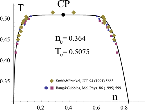
Figure 1: Fitting the binodal of two dimensional LJ fluid (3) with $z=1/3$, $T_{Z}=2.03$ and $n_{b}=0.971$ to the results of the simulations Singh et al. (1990); Jiang and Gubbins (1995). Also the corresponding locus of the CP is shown.

The same procedure can be applied to the $3D$ case. Here we use the results of Talapov and Blote (1996) for the $3D$ Ising model. There data for the spontaneous magnetization $M(t)=2x(t)-1$ were described by the expression:

$$x=\frac{1}{2}\left(1\pm\tau^{\beta}\left(b_{0}+a_{1}\tau+a_{\Delta_{1}}\,\tau^{\Delta_{1}}\right)\right)\,,\quad\tau=1-t\,,$$ (11)

where $\beta=0.326941\,,\Delta_{1}=0.50842$, $b_{0}=1.6919\,,a_{1}=-0.42572366\,,a_{\Delta_{1}}=-0.34357731$. This expression represents the data in the region $0.0005<\tau<0.26$. So we use (11) as the “true“ binodal of the $3D$ LG. From the other side for the real molecular fluids the Guggenheim’s Guggenheim (1945) empirical expressions:

$$\frac{n_{l,\,g}}{n_{c}}=1+\frac{3}{4}\,\left(\,1-T/T_{c}\,\right)\pm\frac{7}{4}\,\left(\,1-T/T_{c}\,\right)^{1/3}\,.$$ (12)

are well known.

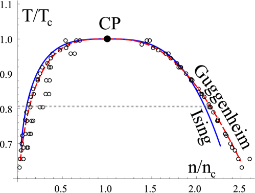
Figure 2: Binodal for $3D$ LJ fluid (blue line) obtained from (11) the mapping after transformation (3) with $z=1/2$, $T_{Z}=T_{B}^{(vdW)}=4$. The grey dashed line shows the range of applicability of (11). The red line is for the Guggenheim binodal (12). Circles are for the data Dunikov et al. (2001); Ou-Yang et al. (2005) (different circles at a given temperature in the gas branch are for different total number of particles in simulations of Dunikov et al. (2001)).

In Fig. 2 the result of transformation of the Ising binodal (11) is shown. The mapping of the Ising model quite satisfactory correlates with the data near the CP ($\tau<0.1$), while the Guggenheim curve better reproduce the data in outer region far from the CP.

Note that both (11) and (12) do not account for the diameter singularity of the density Buckingham (1972); *crit_diamgreermold_annrevpc1981; *crit_diamexp_annrevchemphys1986. The possibility to apply the transformation (3) directly to the results of simulations of LJ fluids is facilitated by the fact that it neglects the singular fluctuational corrections to the regular behavior of the diameter. According to the theoretical approaches Rehr and Mermin (1973); Kim et al. (2003); Kulinskii and Malomuzh (2009) the diameter of the density of the molecular liquid has the following structure:

$$n_{d}=\frac{n_{l}+n_{g}}{2\,n_{c}}-1=D_{2\beta}\,|\tau|^{2\beta}+D_{1-\alpha}\,|\tau|^{1-\alpha}+D_{1}\,|\tau|+\ldots$$ (13)

To the best of our knowledge none of the leading singular terms $\tau^{\beta}$ or $\tau^{1-\alpha}$ has never been discussed in computer simulations. According to Okumura and Yonezawa (2000) the diameter anomaly is difficult to observe by molecular simulations. The data of computer simulations Smit and Frenkel (1991); Lotfi et al. (1992); Wilding (1995); Okumura and Yonezawa (2000); Camp and Patey (2001); Ou-Yang et al. (2005); Duda et al. (2007) are claimed to be consistent with the law of rectilinear diameter and commonly, the locus of the CP is obtained by the extrapolation of the data from the two-phase region using the classical rectilinear diameter law. Then the value $n_{c}$ is greatly influenced by the form of such extrapolation in view of wide opening of the binodal.

It seems evident that LJ fluid does not possess any particle-hole symmetry which lead to regular diameter and the density variable should display both anomalies in its diameter as it does in the case of real and model fluids Greer et al. (1983); *liqmetals_singdiamhensel_prl1985; *crit_aniswangasymmetry_pre2007. The results obtained for real substances show that $\left|D_{1-\alpha}/D_{2\beta}\right|\gtrsim 10$ Kim and Fisher (2005); Wang and Anisimov (2007). So at least $|\tau|^{1-\alpha}$ anomaly may be observed. This poses the problem as to the values of the critical amplitudes $D_{2\beta},\,D_{1-\alpha}$ and their dependence on the microscopic interactions. This question needs further investigation.

As a summary we have demonstrated the usefulness of the transformation (3) in order to get the binodal of LJ fluid. By this we also confirmed the adequacy of the construction of the linear element (4) as the key point in construction of the isomorphism transformation (3). This gives the alternative to the commonly used Zeno-line based considerations Ben-Amotz and Herschbach (1990); Apfelbaum et al. (2006).

References

- Baxter (2007) R. J. Baxter, Exactly Solved Models in Statistical Mechanics (Dover Publications, 2007) ISBN 0486462714.
- Kulinskii (2010) V. L. Kulinskii, Journal of Physical Chemistry B, 114, 2852 (2010a).
- Powles (1983) J. G. Powles, Journal of Physics C: Solid State Physics, 16, 503 (1983).
- Ben-Amotz and Herschbach (1990) D. Ben-Amotz and D. R. Herschbach, Israel Journal of Chemistry, 30, 59 (1990).
- Apfelbaum et al. (2006) E. M. Apfelbaum, V. S. Vorob’ev, and G. A. Martynov, Journal of Physical Chemistry B, 110, 8474 (2006).
- Apfelbaum and Vorob’ev (2008) E. M. Apfelbaum and V. S. Vorob’ev, J. Phys. Chem B., 112, 13064 (2008).
- Hansen and Mcdonald (2006) J.-P. Hansen and I. R. Mcdonald, Theory of Simple Liquids, Third Edition (Academic Press, 2006) ISBN 0123705355.
- Kulinskii (2010) V. L. Kulinskii, The Journal of Chemical Physics, 133, 034121 (2010b).
- Onsager (1944) L. Onsager, Phys. Rev., 65, 117 (1944).
- Jiang and Gubbins (1995) S. Jiang and K. E. Gubbins, Molecular Physics: An International Journal at the Interface Between Chemistry and Physics, 86, 599 (1995).
- Singh et al. (1990) R. R. Singh, K. S. Pitzer, J. J. de Pablo, and J. M. Prausnitz, The Journal of Chemical Physics, 92, 5463 (1990).
- Talapov and Blote (1996) A. L. Talapov and H. W. J. Blote, Journal of Physics A: Mathematical and General, 29, 5727 (1996).
- Guggenheim (1945) E. A. Guggenheim, The Journal of Chemical Physics, 13, 253 (1945).
- Dunikov et al. (2001) D. O. Dunikov, S. P. Malyshenko, and V. V. Zhakhovskii, The Journal of Chemical Physics, 115, 6623 (2001).
- Ou-Yang et al. (2005) W. Z. Ou-Yang, Z.-Y. Lu, T.-F. Shi, Z.-Y. Sun, and L.-J. An, The Journal of Chemical Physics, 123, 254502 (2005).
- Buckingham (1972) M. J. Buckingham, in Phase Transitions and Critical Phenomena, Vol. 2, edited by C. Domb and M. S. Green (Academic, London, London, 1972) Chap. Thermodynamics, p. 18.
- Greer and Moldover (1981) S. Greer and M. Moldover, Ann. Rev. Phys. Chem., 32, 233 265 (1981).
- Sengers and Sengers (1986) J. V. Sengers and J. M. H. L. Sengers, Annual Review of Physical Chemistry, 37, 189 (1986).
- Rehr and Mermin (1973) J. J. Rehr and N. D. Mermin, Physical Review A, 8, 472 (1973).
- Kim et al. (2003) Y. C. Kim, M. E. Fisher, and G. Orkoulas, Physical Review E: Statistical, Nonlinear, and Soft Matter Physics, 67, 061506 (2003).
- Kulinskii and Malomuzh (2009) V. Kulinskii and N. Malomuzh, Physica A: Statistical Mechanics and its Applications, 388, 621 (2009), ISSN 03784371.
- Okumura and Yonezawa (2000) H. Okumura and F. Yonezawa, The Journal of Chemical Physics, 113, 9162 (2000).
- Smit and Frenkel (1991) B. Smit and D. Frenkel, The Journal of Chemical Physics, 94, 5663 (1991).
- Lotfi et al. (1992) A. Lotfi, J. Vrabec, and J. Fischer, Molecular Physics: An International Journal at the Interface Between Chemistry and Physics, 76, 1319 (1992).
- Wilding (1995) N. B. Wilding, Physical Review E: Statistical, Nonlinear, and Soft Matter Physics, 52, 602 (1995).
- Camp and Patey (2001) P. J. Camp and G. N. Patey, The Journal of Chemical Physics, 114, 399 (2001).
- Duda et al. (2007) Y. Duda, A. Romero-Martínez, and P. Orea, The Journal of Chemical Physics, 126, 224510 (2007).
- Greer et al. (1983) S. C. Greer, B. K. Das, A. Kumar, and E. S. R. Gopal, The Journal of Chemical Physics, 79, 4545 (1983).
- Jüngst et al. (1985) S. Jüngst, B. Knuth, and F. Hensel, Phys. Rev. Lett., 55, 2160 (1985).
- Wang and Anisimov (2007) J. Wang and M. A. Anisimov, Physical Review E (Statistical, Nonlinear, and Soft Matter Physics), 75, 051107 (2007).
- Kim and Fisher (2005) Y. Kim and M. Fisher, Chemical Physics Letters, 414, 185 (2005).