Analytical potential-density pairs for bars

Abstract

An identity that relates multipolar solutions of the Einstein equations to Newtonian potentials of bars with linear densities proportional to Legendre polynomials is used to construct analytical potential-density pairs of infinitesimally thin bars with a given linear density profile. By means of a suitable transformation, softened bars that are free of singularities are also obtained. As an application we study the equilibrium points and stability for the motion of test particles in the gravitational field for three models of rotating bars.

Key words: galaxies: kinematics and dynamics

1 Introduction

Bars are a common self-gravitating structure present in disc galaxies. About 50% of such galaxies are stongly or weakly barred, including our Milky Way [1, 2]. The effect of a weak bar is usually represented as a potential in cylindrical coordinates in the form $\Phi(R,\varphi)=\Phi(R)\cos(2\varphi)$ [3]. In the case of strong bars, the only exact, self-consistent models known are those of Freeman [4], although they present some unrealistic features for bars. In studies of orbits involving strong bars, they are often modelled as homogeneous ellipsoids [5, 6] or inhomogeneous prolate spheroids [7, 8, 9, 10]. These mass distributions have a finite extent. Long & Murali [11] discuss a simple method to generate analytical potential-density pairs for barred systems that extend to all space.

In this paper we construct analytical potential-density pairs for infinitesimally thin and ‘softened’ bars [11] that can be expressed solely in terms of elementary functions. The starting point is an identity that relates multipolar solutions of the Einstein equations to Newtonian potentials of bars with densities proportional to Legendre polynomials. These bars can then be superposed to generate other bars with a desired density profile. We also use the method of [11] to soften the infinitesimally thin bars. This is presented in Section 2. In Section 3 the potentials for barred systems are used to study an aspect of the motion of test particles in uniform rotating bars, namely the equilibrium points (Lagrange points) and their stability. We relate the properties of the equilibrium points to the mass distribution of the bar models. Section 4 is devoted to the discussion of the results.

2 Bars with variable densities

In this section an identity derived by Letelier [12] will be used as a starting point to construct potential-density pairs of bars with various linear density profiles. The Newtonian potential of a bar of length $2L$ with linear density $\lambda(z)$ located symmetrically along the $z$-axis is

$$\Phi=-G\int_{-L}^{L}\frac{\lambda(z^{\prime})\mathrm{d}z^{\prime}}{\sqrt{R^{2}+\left(z-z^{\prime}\right)^{2}}}\mbox{,}$$ (1)

where $G$ is the gravitational constant. Letelier [12] found the following identity:

$$Q_{n}(\xi)P_{n}(\eta)=\frac{1}{2}\int_{-L}^{L}\frac{P_{n}(z^{\prime}/L)\mathrm{d}z^{\prime}}{\sqrt{R^{2}+\left(z-z^{\prime}\right)^{2}}}\mbox{,}$$ (2)

where $P_{n}$ and $Q_{n}$ are, respectively, the Legendre polynomials and the Legendre functions of the second kind and $(\xi,\eta)$ are the spheroidal coordinates related to the cylindrical coordinates $(R,z)$ through

$$\xi=(R_{1}+R_{2})/(2L)\text{,}\qquad\eta=(R_{1}-R_{2})/(2L)\mbox{,}$$ (3)

$$R_{1}=\sqrt{R^{2}+\left(z+L\right)^{2}}\text{,}\qquad R_{2}=\sqrt{R^{2}+\left(z-L\right)^{2}}\mbox{,}$$ (4)

with $\xi\geq 1$ and $-1\leq\eta\leq 1$. Comparing equations (1) and (2), and introducing the mass $M$, we see that relation (2) represents a family of bars with linear density

$$\lambda_{n}(z)=\frac{M}{2L}P_{n}(z/L)\mbox{,}$$ (5)

associated with a potential $\Phi_{n}=-GMQ_{n}(\xi)P_{n}(\eta)/L$.

Since the Legendre polynomials form a complete set of functions, the members of the family (5) can be superposed to generate potential-density pairs for bars with a prescribed density distribution. The simplest case is the bar with constant density

$$\lambda_{0}=\frac{M}{2L}\mbox{,}$$ (6)

whose potential can be expressed in cylindrical coordinates as

$$\Phi_{0}=\frac{GM}{2L}\ln\left[\frac{z-L+\sqrt{R^{2}+\left(z-L\right)^{2}}}{z+L+\sqrt{R^{2}+\left(z+L\right)^{2}}}\right]\mbox{.}$$ (7)

To obtain the simple form of equation (7) from the Legendre function $Q_{0}$ we used the auxiliar functions $\mu_{1}=z+L+R_{1}$, $\mu_{2}=z-L+R_{2}$ and the identities [13]

$$R_{1}=\frac{R^{2}+\mu_{1}^{2}}{2\mu_{1}}\text{,}\qquad R_{2}=\frac{R^{2}+\mu_{2}^{2}}{2\mu_{2}}\mbox{,}$$ (8)

$$z+L=\frac{\mu_{1}^{2}-R^{2}}{2\mu_{1}}\text{,}\qquad z-L=\frac{\mu_{2}^{2}-R^{2}}{2\mu_{2}}\mbox{.}$$ (9)

A bar with maximum of density at the centre and vanishing density at both ends can be obtained by the superposition

$$\lambda_{02}=\lambda_{0}-\lambda_{2}=\frac{3M}{4L}\left(1-\frac{z^{2}}{L^{2}}\right)\mbox{.}$$ (10)

The corresponding potential reads

$$\Phi_{02}=\frac{3GM}{8L^{3}}\left(R^{2}+2L^{2}-2z^{2}\right)\ln\left[\frac{z-L+\sqrt{R^{2}+\left(z-L\right)^{2}}}{z+L+\sqrt{R^{2}+\left(z+L\right)^{2}}}\right]\\ +\frac{3GM}{8L^{3}}\left[\left(L-3z\right)\sqrt{R^{2}+\left(z+L\right)^{2}}+\left(L+3z\right)\sqrt{R^{2}+\left(z-L\right)^{2}}\right]\mbox{.}$$ (11)

We will also consider another bar with density obtained by the superposition

$$\lambda_{024}=\lambda_{0}+\frac{5}{7}\lambda_{2}-\frac{12}{7}\lambda_{4}=\frac{15Mz^{2}}{4L^{3}}\left(1-\frac{z^{2}}{L^{2}}\right)\mbox{.}$$ (12)

The density (12) vanishes at the centre and at both ends of the bar, and has maxima at $z/L=\pm\sqrt{2}/2$. The associated potential can be expressed as

$$\Phi_{024}=\frac{15GM}{32L^{5}}\left(-3R^{4}+24R^{2}z^{2}-4R^{2}L^{2}+8z^{2}L^{2}-8z^{4}\right)\\ \times\ln\left[\frac{z-L+\sqrt{R^{2}+\left(z-L\right)^{2}}}{z+L+\sqrt{R^{2}+\left(z+L\right)^{2}}}\right]+\frac{5GM}{32L^{5}}\left[\left(-55R^{2}z-9R^{2}L+26z^{2}L\right.\right.\\ \left.\left.-22zL^{2}+50z^{3}-6L^{3}\right)\sqrt{R^{2}+\left(z-L\right)^{2}}\right.\\ \left.+\left(55R^{2}z-9R^{2}L+26z^{2}L+22zL^{2}-50z^{3}-6L^{3}\right)\sqrt{R^{2}+\left(z+L\right)^{2}}\right]\mbox{.}$$ (13)

The above potential-density pairs refer to infinitesimally thin bars, thus the potential is singular along the bar. For astrophysical applications (e.g. galactic bars) more realistic potentials should be free of singularities. A very simple way to ‘soften’ these potentials is by making a Plummer-like transformation $R^{2}\rightarrow R^{2}+b^{2}$, where $b$ is a non-negative parameter [11]. With this procedure one obtains potential density-pairs that make a transition between infinitesimally thin bars $(b=0)$ and a Plummer sphere $(b\gg L)$ [3]. Applying this transformation on the potentials (7), (11) and (13), the corresponding mass density distributions are calculated directly from Poisson equation in cylindrical coordinates,

$$\Phi_{,RR}+\frac{\Phi_{,R}}{R}+\Phi_{,zz}=4\pi G\rho\mbox{.}$$ (14)

The explicit expressions are given in Appendix A. The three mass densities are free from singularities and non-negative everywhere. For large values of $R$ and $z$, the mass densities decay with $(R^{2}+z^{2})^{-5/2}$, as can be verified by an asymptotic expansion or simply by noting that in this limit the densities approach that of the Plummer sphere, which decays as $(R^{2}+z^{2})^{-5/2}$. Thus, in principle, they fall fast enough to put a clear cut-off and consider them as finite. In Figs 1(a) and (b) we show some isodensity contours of the dimensionless density $\bar{\rho}_{0}=\rho_{0}/(M/L^{3})$, equation (40), as functions of $R/L$ and $z/L$ for a ‘softening parameter’ $b/L=0.25$ in Fig. 1(a) and $b/L=0.75$ in Fig. 1(b). Figs 2(a) and (b) and Figs 3(a) and (b) display, respectively, isodensity contours of the other dimensionless barred densities (42) and (44) for the same values of the parameter $b/L$ as in Figs 1(a) and (b). The softened bars retain the same qualitative characteristics as the infinitesimally thin ones, e.g. the isodensity curves in Figs 1(a) and (b) are more elongated than those displayed in Figs 2(a) and (b), because the linear density of the thin bar (6) is less concentrated at its centre than the density of the thin bar (10).

Figure 1: Isodensity contours of the dimensionless density $\bar{\rho}_{0}=\rho_{0}/(M/L^{3})$, equation (40), as functions of $R/L$ and $z/L$ for (a) $b/L=0.25$ and (b) $b/L=0.75$.

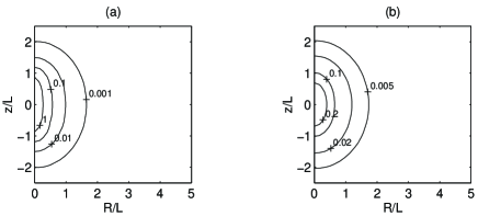
Figure 2: Isodensity contours of the dimensionless density $\bar{\rho}_{02}=\rho_{02}/(M/L^{3})$, equation (42), as functions of $R/L$ and $z/L$ for (a) $b/L=0.25$ and (b) $b/L=0.75$.

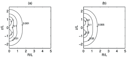
Figure 3: Isodensity contours of the dimensionless density $\bar{\rho}_{024}=\rho_{024}/(M/L^{3})$, equation (44), as functions of $R/L$ and $z/L$ for (a) $b/L=0.25$ and (b) $b/L=0.75$.

3 Equilibrium points and their stability

An important aspect related to the morphology of barred galaxies is the study of motion of a test particle in the gravitational field of a uniform rotating bar. In this section we will discuss the equilibrium points and their stability for the motion in the field of the softened bars discussed in Section 2. For convenience, we place the bar along the $x$-axis, and consider the motion on the $xy$ plane. For this task, the potentials (39), (41) and (43) should be rewritten by replacing $z\rightarrow x$ and $R^{2}\rightarrow y^{2}$. In the forthcoming discussion, we shall refer the potential-density pair (39)–(40) as bar model 1, the pair (41)–(42) as bar model 2 and the pair (43)–(44) as bar model 3.

In a coordinate system attached to the bar that rotates with an (constant) angular velocity $\Omega$, the equations of motion of a test particle are

$$\ddot{x}-2\Omega\dot{y} =-\frac{\partial\Phi_{eff.}}{\partial x}\mbox{,}$$ (15)

$$\ddot{y}+2\Omega\dot{x} =-\frac{\partial\Phi_{eff.}}{\partial y}\mbox{,}$$ (16)

where dots indicate derivatives with respect to time, and $\Phi_{eff.}$ is the ‘effective’ potential,

$$\Phi_{eff.}=\Phi_{bar}-\frac{\Omega^{2}}{2}\left(x^{2}+y^{2}\right)\mbox{.}$$ (17)

At an equilibrium point, $\vec{\nabla}\Phi_{eff.}=0$, and the resulting system of two algebraic equations must be solved to obtain the equilibrium points (Lagrange points). Because of the symmetry of the models, the equilibrium points are symmetric with respect to the $x$- and $y$-axes. One Lagrange point is the origin $(0,0)$, the pair on the $x$-axis will have coordinates $(\pm x_{L},0)$ and the pair on the $y$-axis will have coordinates $(0,\pm y_{L})$. The stability of an equilibrium point is determined by the linearized equations of motion around it. The following conditions are necessary and sufficient for an equilibrium point be stable [3]:

$$\alpha\beta>0\mbox{,}$$ (18)

$$-\left(\alpha+\beta+4\Omega^{2}\right)<0\mbox{,}$$ (19)

$$\left(\alpha+\beta+4\Omega^{2}\right)^{2}-4\alpha\beta>0\mbox{,}$$ (20)

and

$$\alpha=\left(\frac{\partial^{2}\Phi_{eff.}}{\partial x^{2}}\right)_{eq.}\text{,}\qquad\beta=\left(\frac{\partial^{2}\Phi_{eff.}}{\partial y^{2}}\right)_{eq.}\mbox{,}$$ (21)

where the second derivatives are evaluated at an equilibrium point. We shall calculate and analyse the stability of the Lagrange points for each of the three models of bars.

3.1 Bar model 1

At the origin the values of the second derivatives (21) are

$$\alpha=\frac{GM}{\left(b^{2}+L^{2}\right)^{3/2}}-\Omega^{2}\text{,}\qquad\beta=\frac{GM}{b^{2}\sqrt{b^{2}+L^{2}}}-\Omega^{2}\mbox{.}$$ (22)

One finds analytically that conditions (19) and (20) are always satisfied. By condition (18), the origin will be unstable for angular velocities in the range

$$\sqrt{\frac{GM}{\left(b^{2}+L^{2}\right)^{3/2}}}<\Omega<\sqrt{\frac{GM}{b^{2}\sqrt{b^{2}+L^{2}}}}\mbox{.}$$ (23)

Fig. 4(a) shows the stability diagram of the point $(0,0)$, as functions of $b/L$ and of the dimensionless angular velocity $\bar{\Omega}=\Omega/\sqrt{GM/L^{3}}$. The unstable region grows as the bar becomes more elongated.

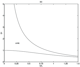
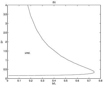
Figure 4: (a) Stability diagram of the equilibrium point $(0,0)$ for bar model 1 as functions of $b/L$ and $\bar{\Omega}=\Omega/\sqrt{GM/L^{3}}$. (b) Stability diagram of the equilibrium point $(0,y_{L}/L)$ for bar model 1 as functions of $b/L$ and $\bar{\Omega}=\Omega/\sqrt{GM/L^{3}}$.

On the $y$-axis the equilibrium point is given by the equation

$$\frac{GM}{\left(y_{L}^{2}+b^{2}\right)\sqrt{y_{L}^{2}+b^{2}+L^{2}}}-\Omega^{2}=0\mbox{.}$$ (24)

In this case the stability is better investigated by a graphical analysis of conditions (18)–(20). Fig. 4(b) displays the stability diagram of the Lagrange points on the $y$-axis as functions of $b/L$ and $\bar{\Omega}$. For $b/L\gtrapprox 0.75$ the points are stable for all values of the angular velocity. For lower values of $b/L$ there is an interval of $\bar{\Omega}$ where the equilibrium points are unstable and this interval becomes larger as $b/L$ approaches zero. In this limit, the points are stable for an angular velocity less than

$$\bar{\Omega}=\frac{13\sqrt{2}-18}{14}\sqrt{5+4\sqrt{2}}\sqrt{2+\sqrt{2}}\approx 0.166\mbox{.}$$ (25)

Figure 5: (a) Curves of equation (26) for some values of $b/L$. (b) The stability of the equilibrium point(s) $(x_{L}/L,0)$ for bar model 1 as function of $b/L$.

The equilibrium points on the $x$-axis are given by the equation

$$\frac{GM\left[\sqrt{b^{2}+\left(x_{L}+L\right)^{2}}-\sqrt{b^{2}+\left(x_{L}-L\right)^{2}}\right]}{2L\sqrt{b^{2}+\left(x_{L}-L\right)^{2}}\sqrt{b^{2}+\left(x_{L}+L\right)^{2}}}-\Omega^{2}x_{L}=0$$ (26)

For a given value of $\Omega$ the equilibrium point must be found by solving (26) numerically. On the other hand, for a given value of $x_{L}$ one might calculate $\Omega$ directly from (26). In Fig. 5(a) we plot some curves of $\bar{\Omega}$ as function of $x_{L}/L$ for some values of the parameter $b/L$. It is seen that there may exist two equilibrium points for a given value of the angular velocity, which means two pairs of Lagrange points on the $x$-axis. This can happen for values of $b/L\lessapprox 0.82$. Fig. 5(b) shows the stability of the equilibrium point(s) $(x_{L}/L,0)$ as function of $b/L$. Comparing Figs 5(a) and (b), we note that when two equilibrium points exist, the inner point is always stable, whereas the outer is unstable. When only one equilibrium point exists, it is always unstable.

3.2 Bar model 2

For this model of bar, the values of the second derivatives (21) at the origin read

$$\alpha=-\frac{3GM}{2L^{3}}\ln\left(\frac{\sqrt{b^{2}+L^{2}}-L}{\sqrt{b^{2}+L^{2}}+L}\right)-\frac{3GM}{L^{2}\sqrt{b^{2}+L^{2}}}-\Omega^{2}\mbox{,}$$

$$\beta=\frac{3GM}{4L^{3}}\ln\left(\frac{\sqrt{b^{2}+L^{2}}-L}{\sqrt{b^{2}+L^{2}}+L}\right)+\frac{3GM\sqrt{b^{2}+L^{2}}}{2b^{2}L^{2}}-\Omega^{2}\mbox{.}$$ (27)

The origin will be an unstable equilibrium point for angular velocities in the interval

$$\left[-\frac{3GM}{2L^{3}}\ln\left(\frac{\sqrt{b^{2}+L^{2}}-L}{\sqrt{b^{2}+L^{2}}+L}\right)-\frac{3GM}{L^{2}\sqrt{b^{2}+L^{2}}}\right]^{1/2}<\Omega<\left[\frac{3GM}{4L^{3}}\right.\\ \left.\times\ln\left(\frac{\sqrt{b^{2}+L^{2}}-L}{\sqrt{b^{2}+L^{2}}+L}\right)+\frac{3GM\sqrt{b^{2}+L^{2}}}{2b^{2}L^{2}}\right]^{1/2}\mbox{.}$$ (28)

In Fig. 4(a) we display the stability diagram of the point $(0,0)$, as functions of $b/L$ and of the angular velocity $\bar{\Omega}$. Also in this model the unstable region grows as the bar becomes more elongated.

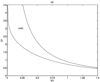
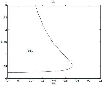
Figure 6: (a) Stability diagram of the equilibrium point $(0,0)$ for bar model 2 as functions of $b/L$ and $\bar{\Omega}=\Omega/\sqrt{GM/L^{3}}$. (b) Stability diagram of the equilibrium point $(0,y_{L}/L)$ for bar model 2 as functions of $b/L$ and $\bar{\Omega}=\Omega/\sqrt{GM/L^{3}}$.

On the $y$-axis the equilibrium point is given by the equation

$$\frac{3GM}{4L^{3}}\ln\left(\frac{\sqrt{y_{L}^{2}+b^{2}+L^{2}}-L}{\sqrt{y_{L}^{2}+b^{2}+L^{2}}+L}\right)+\frac{3GM\sqrt{y_{L}^{2}+b^{2}+L^{2}}}{2L^{2}\left(y_{L}^{2}+b^{2}\right)}-\Omega^{2}=0\mbox{.}$$ (29)

The stability diagram of the Lagrange points on the $y$-axis is displayed in Fig. 6(b). For $b/L\gtrapprox 0.56$ the points are stable for all values of the angular velocity. In the limit of infinitesimally thin bar, the points are stable for $\bar{\Omega}\lessapprox 0.25$.

The equilibrium point on the $x$-axis is calculated from

$$-\frac{3GM}{2L^{3}}\ln\left[\frac{x_{L}-L+\sqrt{b^{2}+\left(x_{L}-L\right)^{2}}}{x_{L}+L+\sqrt{b^{2}+\left(x_{L}+L\right)^{2}}}\right]\\ -\frac{3GM}{2x_{L}L^{3}}\left[\sqrt{b^{2}+\left(x_{L}+L\right)^{2}}-\sqrt{b^{2}+\left(x_{L}-L\right)^{2}}\right]-\Omega^{2}=0\mbox{.}$$ (30)

In this case there exists only one equilibrium point for a given value of the angular velocity, and we found that this point is always unstable.

3.3 Bar model 3

For bar model 3, the values of the second derivatives (21) at the origin read

$$\alpha=\frac{15GM\left(3b^{2}+L^{2}\right)}{2L^{5}}\ln\left(\frac{\sqrt{b^{2}+L^{2}}-L}{\sqrt{b^{2}+L^{2}}+L}\right)+\frac{15GM\left(3b^{2}+2L^{2}\right)}{L^{4}\sqrt{b^{2}+L^{2}}}-\Omega^{2}\mbox{,}$$ (31)

$$\beta=-\frac{15GM\left(3b^{2}+2L^{2}\right)}{8L^{5}}\ln\left(\frac{\sqrt{b^{2}+L^{2}}-L}{\sqrt{b^{2}+L^{2}}+L}\right)-\frac{45GM\sqrt{b^{2}+L^{2}}}{4L^{4}}-\Omega^{2}\mbox{.}$$ (32)

The origin will be an unstable equilibrium point for angular velocities in the interval $\Omega_{1}<\Omega<\Omega_{2}$, where

$$\Omega_{1}=\left[\frac{15GM\left(3b^{2}+L^{2}\right)}{2L^{5}}\ln\left(\frac{\sqrt{b^{2}+L^{2}}-L}{\sqrt{b^{2}+L^{2}}+L}\right)+\frac{15GM\left(3b^{2}+2L^{2}\right)}{L^{4}\sqrt{b^{2}+L^{2}}}\right]^{1/2}\mbox{,}$$ (33)

$$\Omega_{2}=\left[-\frac{15GM\left(3b^{2}+2L^{2}\right)}{8L^{5}}\ln\left(\frac{\sqrt{b^{2}+L^{2}}-L}{\sqrt{b^{2}+L^{2}}+L}\right)-\frac{45GM\sqrt{b^{2}+L^{2}}}{4L^{4}}\right]^{1/2}\mbox{.}$$ (34)

Furthermore, there is another region of instability for angular velocities greater then $\Omega=\sqrt{A/B}$, where

$$A=-\frac{2025G^{2}M^{2}\left(5b^{2}+2L^{2}\right)^{2}}{64L^{10}}\ln^{2}\left(\frac{\sqrt{b^{2}+L^{2}}-L}{\sqrt{b^{2}+L^{2}}+L}\right)$$

$$-\frac{675G^{2}M^{2}\left(75b^{4}+85b^{2}L^{2}+22L^{4}\right)}{16L^{9}\sqrt{b^{2}+L^{2}}}\ln\left(\frac{\sqrt{b^{2}+L^{2}}-L}{\sqrt{b^{2}+L^{2}}+L}\right)$$

$$-\frac{225G^{2}M^{2}\left(15b^{2}+11L^{2}\right)^{2}}{16L^{8}\left(b^{2}+L^{2}\right)}\mbox{,}$$ (35)

$$B=\frac{15GM\left(9b^{2}+2L^{2}\right)}{L^{5}}\ln\left(\frac{\sqrt{b^{2}+L^{2}}-L}{\sqrt{b^{2}+L^{2}}+L}\right)+\frac{30GM\left(9b^{2}+5L^{2}\right)}{L^{4}\sqrt{b^{2}+L^{2}}}\mbox{.}$$ (36)

Figs 7(a) and (b) show the stability diagram of the point $(0,0)$, as functions of $b/L$ and the angular velocity $\bar{\Omega}$. Fig. 7(b) gives an enlarged view of the second region of instability.

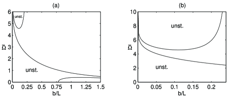
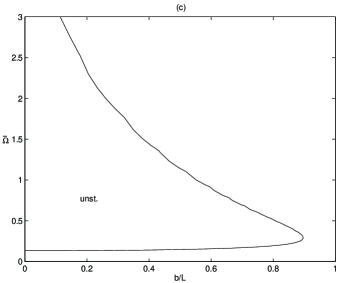
Figure 7: (a)–(b) Stability diagram of the equilibrium point $(0,0)$ for bar model 3 as functions of $b/L$ and $\bar{\Omega}=\Omega/\sqrt{GM/L^{3}}$. (c) Stability diagram of the equilibrium point $(0,y_{L}/L)$ for bar model 3 as functions of $b/L$ and $\bar{\Omega}=\Omega/\sqrt{GM/L^{3}}$.

On the $y$-axis the equilibrium point is given by the relation

$$-\frac{15GM\left(3y_{L}^{2}+3b^{2}+2L^{2}\right)}{8L^{5}}\ln\left(\frac{\sqrt{y_{L}^{2}+b^{2}+L^{2}}-L}{\sqrt{y_{L}^{2}+b^{2}+L^{2}}+L}\right)\\ -\frac{45GM\sqrt{y_{L}^{2}+b^{2}+L^{2}}}{4L^{4}}-\Omega^{2}=0\mbox{.}$$ (37)

The stability diagram of the Lagrange points on the $y$-axis is displayed in Fig. 7(c). For $b/L\gtrapprox 0.90$ the points are stable for all values of the angular velocity. In the limit of infinitesimally thin bar, the points are stable for $\bar{\Omega}\lessapprox 0.13$.

The equilibrium point on the $x$-axis is calculated from

$$\frac{15GM\left(3b^{2}+L^{2}-2x_{L}^{2}\right)}{2L^{5}}\ln\left[\frac{x_{L}-L+\sqrt{b^{2}+\left(x_{L}-L\right)^{2}}}{x_{L}+L+\sqrt{b^{2}+\left(x_{L}+L\right)^{2}}}\right]\\ +\frac{5GM}{2x_{L}L^{5}}\left\{\left(4b^{2}+L^{2}-11x_{L}^{2}\right)\left[\sqrt{b^{2}+\left(x_{L}+L\right)^{2}}-\sqrt{b^{2}+\left(x_{L}-L\right)^{2}}\right]\right.\\ \left.+5Lx_{L}\left[\sqrt{b^{2}+\left(x_{L}+L\right)^{2}}+\sqrt{b^{2}+\left(x_{L}-L\right)^{2}}\right]\right\}-\Omega^{2}=0\mbox{.}$$ (38)

Fig. 8(a) shows some curves of $\bar{\Omega}$ as function of $x_{L}/L$ for some values of the parameter $b/L$. As happened with bar model 1, there may also exist two pairs of equilibrium points on the $x$-axis. This is possible for values of $b/L\lessapprox 1.63$. Fig. 8(b) shows the stability of the equilibrium point(s) $(x_{L}/L,0)$ as function of $b/L$. Also here, when two equilibrium points exist, the inner point is always stable, whereas the outer is unstable. When only one equilibrium point exists, it is always unstable.

From Fig. 8(a) we note a particular feature of this model of bar: even without rotation $(\bar{\Omega}=0)$, there is an equilibrium point along the $x$-axis for some values of the parameter $b/L$ (for instance, $x/L\approx 0.6$ for $b/L=0.25$). This static equilibrium point exists because the mass density of the bar is not concentrated at the origin (see Fig. 3). In Fig. 8(b) the dashed curve indicates the location of this point as function of $b/L$. A similar static equilibrium point was found in potential-density pairs for flat rings [14].

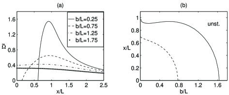
Figure 8: (a) Curves of equation (38) for some values of $b/L$. (b) The stability of the equilibrium point(s) $(x_{L}/L,0)$ for bar model 3 as function of $b/L$. The dashed curve indicates the position of the static equilibrium point.

4 Discussion

We presented analytical potential-density pairs for infinitesimally thin and softened bars constructed from an identity that relates multipolar solutions of the Einstein equations to Newtonian potentials of bars with densities proportional to Legendre polynomials. The main advantage of these models is that all potential density-pairs can be explicitly expressed in terms of elementary functions, and bars with a desired density profile can be constructed from the set of densities (5).

As an application of the barred potentials, we calculated the equilibrium points for the motion of test particles in the gravitational field of three models of rotating bars and analysed their stability. The results suggest some conclusions. The equilibrium point $(0,0)$ has the tendency to be more stable in bar model 2, and more unstable in bar model 3. The stability diagrams for the equilibrium points along the $y$-axis have the same qualitative behaviour for the three models of bars. On the other hand, the properties of the equilibrium points along the $x$-axis seem to be quite sensitive to the particular model of bar used. In the case of bar model 2, the points are always unstable, whereas for bar models 1 and 3, there even exists the possibility of two pairs of equilibrium points, one being stable and the other unstable. It is known that the equilibrium points on the $x$-axis of a homogeneous ellipsoid are always unstable [5, 6]. From our three models the bar model 2 has the nearest shape of an ellipsoid, thus it is not surprising that it exhibits similar properties. It seems that barred mass distributions with less mass concentrated around the centre of the bar tend to stabilize the equilibrium points along the $x$-axis. Our results are in qualitative agreement with those obtained by Michalodimitrakis [6], who compared the stability properties of equilibrium points for a homogeneous ellipsoid and for a homogeneous parallelepiped.

Appendix A Potential-density pairs for softened bars

The expressions for the potentials $\Phi$ and mass densities $\rho$ for the softened thin bar potentials (7), (11) and (13) are given by

$$\Phi_{0}=\frac{GM}{2L}\ln\left(\frac{z-L+\mathcal{R}_{2}}{z+L+\mathcal{R}_{1}}\right)\mbox{,}$$ (39)

$$\rho_{0}=\frac{Mb^{2}}{8\pi L\left(R^{2}+b^{2}\right)^{2}\mathcal{R}_{1}^{3}\mathcal{R}_{2}^{3}}\left\{\mathcal{R}_{2}^{3}\left(z+L\right)\left[3\left(R^{2}+b^{2}\right)+2\left(z+L\right)^{2}\right]\right.$$

$$\left.-\mathcal{R}_{1}^{3}\left(z-L\right)\left[3\left(R^{2}+b^{2}\right)+2\left(z-L\right)^{2}\right]\right\}\mbox{,}$$ (40)

$$\Phi_{02}=\frac{3GM}{8L^{3}}\left(R^{2}+b^{2}+2L^{2}-2z^{2}\right)\ln\left(\frac{z-L+\mathcal{R}_{2}}{z+L+\mathcal{R}_{1}}\right)$$

$$+\frac{3GM}{8L^{3}}\left[\left(L-3z\right)\mathcal{R}_{1}+\left(L+3z\right)\mathcal{R}_{2}\right]\mbox{,}$$ (41)

$$\rho_{02}=\frac{3Mb^{2}}{8\pi L^{3}\left(R^{2}+b^{2}\right)^{2}\mathcal{R}_{1}\mathcal{R}_{2}}\left[\left(R^{2}+b^{2}\right)\left(\mathcal{R}_{1}-\mathcal{R}_{2}\right)z+\mathcal{R}_{1}\left(z-L\right)^{2}\left(z+L\right)\right.$$

$$\left.-\mathcal{R}_{2}\left(z+L\right)^{2}\left(z-L\right)\right]\mbox{,}$$ (42)

$$\Phi_{024}=\frac{15GM}{32L^{5}}\left[-3\left(R^{2}+b^{2}\right)^{2}+24\left(R^{2}+b^{2}\right)z^{2}-4\left(R^{2}+b^{2}\right)L^{2}+8z^{2}L^{2}\right.$$

$$\left.-8z^{4}\right]\ln\left(\frac{z-L+\mathcal{R}_{2}}{z+L+\mathcal{R}_{1}}\right)+\frac{5GM}{32L^{5}}\left\{\left[-55\left(R^{2}+b^{2}\right)z-9\left(R^{2}+b^{2}\right)L\right.\right.$$

$$\left.\left.+26z^{2}L-22zL^{2}+50z^{3}-6L^{3}\right]\mathcal{R}_{2}\right.$$

$$\left.+\left[55\left(R^{2}+b^{2}\right)z-9\left(R^{2}+b^{2}\right)L+26z^{2}L+22zL^{2}-50z^{3}-6L^{3}\right]\mathcal{R}_{1}\right\}\mbox{,}$$ (43)

$$\rho_{024}=\frac{45Mb^{2}}{16\pi L^{5}}\ln\left(\frac{z-L+\mathcal{R}_{2}}{z+L+\mathcal{R}_{1}}\right)+\frac{15Mb^{2}}{16\pi L^{5}\left(R^{2}+b^{2}\right)^{2}\mathcal{R}_{1}\mathcal{R}_{2}}$$

$$\times\left\{\mathcal{R}_{1}\left[\left(R^{2}+b^{2}\right)^{2}\left(5z+3L\right)+\left(R^{2}+b^{2}\right)\left(7z^{3}-5z^{2}L-zL^{2}+L^{3}\right)\right.\right.$$

$$\left.\left.+2z^{2}\left(z+L\right)\left(z-L\right)^{2}\right]+\mathcal{R}_{2}\left[\left(R^{2}+b^{2}\right)^{2}\left(-5z+3L\right)+\left(R^{2}+b^{2}\right)\right.\right.$$

$$\left.\left.\times\left(-7z^{3}-5z^{2}L+zL^{2}+L^{3}\right)-2z^{2}\left(z-L\right)\left(z+L\right)^{2}\right]\right\}\mbox{,}$$ (44)

where $\mathcal{R}_{1}=\sqrt{R^{2}+b^{2}+\left(z+L\right)^{2}}$ and $\mathcal{R}_{2}=\sqrt{R^{2}+b^{2}+\left(z-L\right)^{2}}$.