Three-terminal triple-quantum-dot ring as a charge and spin current rectifier

Abstract

Electronic transport through a triple-quantum-dot ring with three terminals is theoretically studied. By introducing local Rashba spin-orbit interaction on an individual quantum dot, we find that the spin bias in one terminal drives apparent charge currents in the other terminals, accompanied by the similar amplitude and opposite directions of them. Meanwhile, it shows that the characteristics of the spin currents induced by the spin bias are notable. When a magnetic flux is applied through this ring, we see its nontrivial role in the manipulation of the charge and spin currents. With the obtained results, we propose this structure to be a prototype of a charge and spin current rectifier.

I Introduction

The manipulation and control of the behaviors of electron spins in nanostructures have become one subject of intense investigation due to its relevance to quantum computation and quantum information.Ohno ; Dasarma The electron spin in quantum dot (QD) is a natural candidate for the qubit, and then QD is regarded as an elementary cell of quantum computation and quantum information. Therefore, much attention has been paid to the manipulation of the electron spin degree of freedom in QD for its application.Loss ; Loss2 Many schemes have been proposed to work out this problem for obtaining the highly-polarized spin current (in particular, the so-called pure spin current), based on the case of a charge bias between two leads with a magnetic field or the spin-obit (SO) coupling for a QD system.Datta ; Rashba ; Rashba2 ; Sun ; Trocha ; Other Despite these existed works, any new suggestions to realize the highly-polarized spin current are still necessary. Recently, it has been reported that spin bias in leads for mesoscopic systems can be feasible, which, different from the traditional charge bias, induces rich physical phenomena and potential applicationsNagaosa ; Hubner ; Cui ; Li ; Jpn ; LuHZ ; Chi .

In the present work, we choose a three-terminal triple-QD ring, which is feasible to be fabricated by virtue of the current nanoscale and mesoscale technologyNagaosa ; Bao ; Tarucha , to investigate its electron transport properties influenced by the spin bias in one terminal. As a result, by introducing local Rashba spin-orbit interaction on an individual QD, it is found that the spin bias drives apparent charge currents in the two other terminals with interesting properties of them. Besides, the characteristics of the spin currents induced by the spin bias are also notable. With these results, this structure can be proposed to be a prototype of a charge and spin current rectifier.

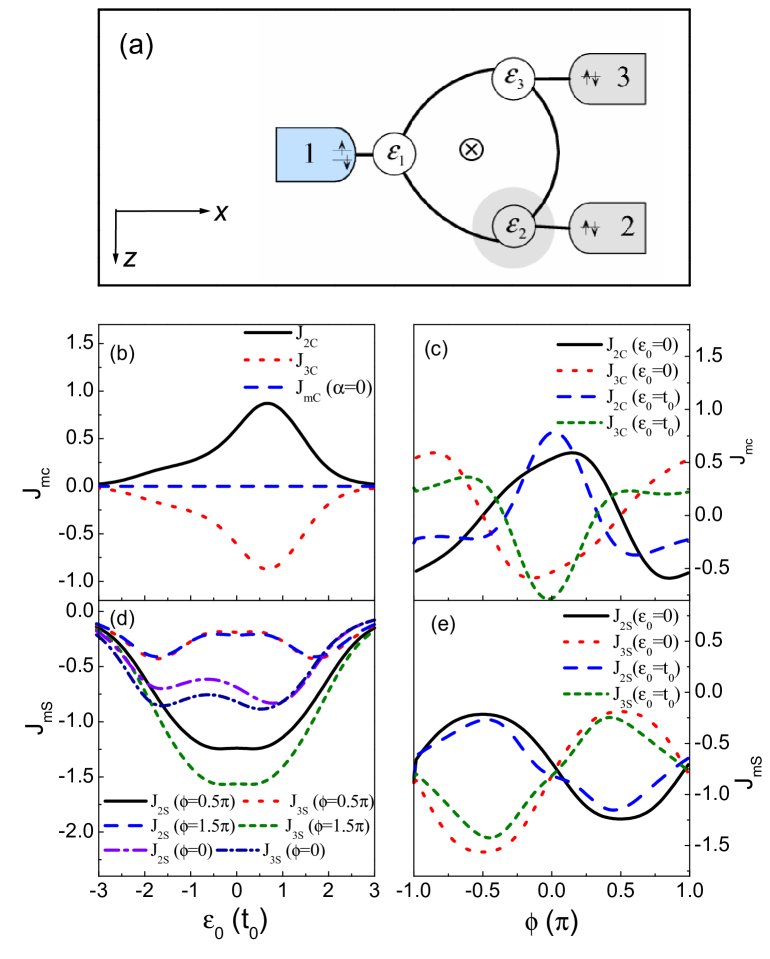
Figure 1: (a) Schematic of a three-terminal triple-QD ring structure with a local Rashba interaction on QD-2. Three QDs and the leads coupling to them are denoted as QD-$j$ and lead-$j$ with $j=1-3$. Spin bias is assumed to be in lead-1. (b) The charge current spectra in lead-2 and lead-3 with the shift of QD levels. (c)The charge currents vs the magnetic phase factor $\phi$. (d) The spin current spectra in lead-2 and lead-3. (e) The spin current spectra vs the magnetic phase factor $\phi$.

II model and formulation

The considered three-terminal triple-QD ring is illustrated in Fig.1(a), which can usually be fabricated by means of split-gate technique in the two-dimensional electron gas. We assume that in one terminal ( lead-1 ) there exists the spin bias $V_{s}$, i.e., the spin-dependent chemical potentials for the spin-up and spin-down electrons are $\mu_{1\sigma}=\varepsilon_{F}+\sigma eV_{s}$.Sun By additionally inserting two normal metallic terminals ( lead-2 and lead-3 ) ( here $\mu_{2\sigma}=\mu_{3\sigma}=\varepsilon_{F}$ ), we would like to observe the charge and spin transport behaviors in the other terminals affected by the spin bias. Correspondingly, if lead-1 is postulated to be the source terminal, the others will be the drain terminals.

In this structure, the Hamiltonian of the electron moving in the x-z plane can be written as $H_{s}=\frac{\textbf{P}^{2}}{2m^{*}}+V(\textbf{r})+\frac{\hat{y}}{2\hbar}\cdot[\alpha(\hat{\sigma}\times\textbf{p})+(\hat{\sigma}\times\textbf{p})\alpha]$, where the potential $V(\textbf{r})$ confines the electron to form the structure geometry, namely, the leads, QDs and the connections. The last term in $H_{s}$ denotes the local Rashba SO coupling on QD-2. For the analysis of the electron properties, we have to second-quantize the above Hamiltonian,gongapl which is composed of three parts: ${\cal H}={\cal H}_{c}+{\cal H}_{d}+{\cal H}_{t}$.

$${\cal H}_{c} =\underset{\sigma jk}{\sum}\varepsilon_{jk\sigma}c_{jk\sigma}^{\dagger}c_{jk\sigma},$$

$${\cal H}_{d} =\sum_{j=1,\sigma}^{3}\varepsilon_{j}d^{\dagger}_{j\sigma}d_{j\sigma}+\sum_{l=1,\sigma}^{2}[t_{l\sigma}d^{\dagger}_{l\sigma}d_{l+1\sigma}+r_{l}(d_{l\downarrow}^{\dagger}d_{l+1\uparrow}$$

$$-d_{l+1\downarrow}^{\dagger}d_{l\uparrow})]+t_{3}e^{i\phi}d^{\dagger}_{3\sigma}d_{1\sigma}+\mathrm{H.c.},$$

$${\cal H}_{t} =\underset{\sigma jk}{\sum}V_{j\sigma}d^{\dagger}_{j\sigma}c_{jk\sigma}+\mathrm{H.c.},$$ (1)

where $c_{jk\sigma}^{\dagger}$ and $d^{{\dagger}}_{j\sigma}$ $(c_{jk\sigma}$ and $d_{j\sigma})$ are the creation (annihilation) operators corresponding to the basis in lead-$j$ and QD-$j$. $\varepsilon_{jk\sigma}$ and $\varepsilon_{j}$ are the single-particle levels. $V_{j\sigma}$ denotes QD-lead coupling strength. The interdot hopping amplitude $t_{l\sigma}=t_{l}\sqrt{1+\tilde{\alpha}^{2}}e^{-i\sigma\varphi}$ ($l=1,2$), where $t_{l}$ is the ordinary transfer integral irrelevant to the Rashba interaction and $\tilde{\alpha}$ is the dimensionless Rashba coefficient with $\varphi=\tan^{-1}\tilde{\alpha}$Serra . $r_{l}$ is a complex quantity representing the strength of interdot spin flip. The phase factor $\phi$ attached to $t_{3}$ accounts for the magnetic flux through the ring. In addition, the many-body effect can be readily incorporated into the above Hamiltonian by adding the Hubbard term ${\cal V}_{e\text{-}e}=\sum_{j\sigma}{\frac{U_{j}}{2}}n_{j\sigma}n_{j\bar{\sigma}}$.

Starting from the second-quantized Hamiltonian, we can now formulate the electronic transport properties. With the nonequilibrium Keldysh Green function technique, the spin-$\sigma$ current flow in lead-$j$ can be written asMeir ; Gong1

$$J_{j\sigma}=\frac{e}{h}\sum_{j^{\prime}\sigma^{\prime}}\int d\omega T_{j\sigma,j^{\prime}\sigma^{\prime}}(\omega)[f_{j\sigma}(\omega)-f_{j^{\prime}\sigma^{\prime}}(\omega)],$$ (2)

where $f_{j\sigma}(\omega)=(\exp{\omega-\mu_{j\sigma}\over k_{B}T}+1)^{-1}$ is the Fermi distribution function in lead-$j$. $T_{j\sigma,j^{\prime}\sigma^{\prime}}(\omega)=4\Gamma_{j\sigma}G^{r}_{j\sigma,j^{\prime}\sigma^{\prime}}(\omega)\Gamma_{j^{\prime}\sigma^{\prime}}G^{a}_{j^{\prime}\sigma^{\prime},j\sigma}(\omega)$ is the transmission function, describing electron tunneling ability between lead-$j$ to lead-$j^{\prime}$. $\Gamma_{j\sigma}=\pi|V_{j\sigma}|^{2}\rho_{j}(\omega)$, the coupling strength between QD-$j$ and lead-$j$, can be usually regarded as a constant. $G^{r}$ and $G^{a}$, the retarded and advanced Green functions, obey the relationship $[G^{r}]=[G^{a}]^{\dagger}$. From the equation-of-motion method, the retarded Green function can be obtained in a matrix form,

$$[G^{r}]^{-1}=$$

$$\left[\begin{array}[]{cccccc}g_{1\uparrow}^{-1}&-t_{1\uparrow}&-t_{3}e^{-i\phi}&0&r^{*}_{1}&0\\ -t^{*}_{1\uparrow}&g_{2\uparrow}^{-1}&-t_{2\uparrow}&-r^{*}_{1}&0&r^{*}_{2}\\ -t_{3}e^{i\phi}&-t^{*}_{2\uparrow}&g_{3\uparrow}^{-1}&0&-r^{*}_{2}&0\\ 0&-r_{1}&0&g_{1\downarrow}^{-1}&-t_{1\downarrow}&-t_{3}e^{-i\phi}\\ r_{1}&0&-r_{2}&-t^{*}_{1\downarrow}&g_{2\downarrow}^{-1}&-t_{2\downarrow}\\ 0&r_{2}&0&-t_{3}e^{i\phi}&-t^{*}_{2\downarrow}&g_{3\downarrow}^{-1}\end{array}\right].$$ (9)

In the above expression, $g_{j\sigma}$ is the Green function of QD-$j$ unperturbed by the other QDs and in the absence of Rashba effect. $g_{j\sigma}=[(z-\varepsilon_{j})\lambda_{j\sigma}+i\Gamma_{j\sigma}]^{-1}$ with $z=\omega+i0^{+}$. $\lambda_{j\sigma}=\frac{z-\varepsilon_{j}-U_{j}}{z-\varepsilon_{j}-U_{j}+U_{j}\langle n_{j\bar{\sigma}}\rangle}$ results from the second-order approximation of the Coulomb interactionZhengHZ , which is reasonable when the system temperature is higher than the Kondo temperature. $\langle n_{j\sigma}\rangle$ can be numerically resolved by the formula $\langle n_{j\sigma}\rangle=-\frac{i}{2\pi}\int d\omega G^{<}_{j\sigma,j\sigma}$ where $G^{<}_{\sigma\sigma}=\sum_{\sigma^{\prime}}[G^{r}]_{\sigma\sigma^{\prime}}[\Sigma^{<}]_{\sigma^{\prime}}[G^{a}]_{\sigma^{\prime}\sigma}$ and $[\Sigma^{<}]_{\sigma}=2\sum_{j}\Gamma_{j\sigma}f_{j\sigma}(\omega)$.

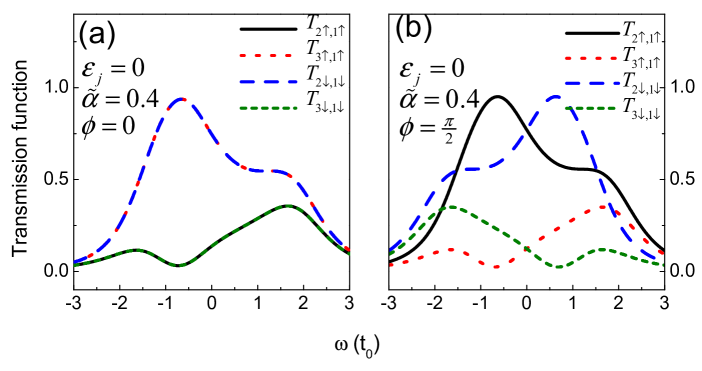
Figure 2: The spectra of transmission functions $T_{m\sigma,1\sigma}$($m$=2,3) with the QD levels fixed at $\varepsilon_{j}=0$. (a) and (b) Zero magnetic field case, and (c)-(d) magnetic phase factor $\phi={\pi\over 2}$.

III Numerical results and discussions

We now proceed on to calculate the charge currents in the drain terminals, lead-2 and lead-3 in this case. Before calculation, the QD-lead couplings are assumed to take the uniform values with $\Gamma_{j\sigma}=t_{0}$, and we consider $t_{0}$ as the energy unit. The structure parameters are for simplicity taken as $|t_{l\sigma}|=t_{3}=t_{0}$, and $\varepsilon_{F}$ is viewed as the energy zero point of this system. Besides, to carry out the numerical calculation, we choose the Rashba coefficient $\tilde{\alpha}=0.4$ which is available in the current experiment.Sarra

We first focus on the electron transport in the linear regime. In this case, the charge current flow is proportional to the linear conductance, i.e., $J_{mc}=\mathcal{G}_{mc}\cdot V_{s}$ ($m=2,3$), where $J_{mc}=J_{m\uparrow}+J_{m\downarrow}$ and the linear charge conductance

$$\mathcal{G}_{mc}=\frac{e^{2}}{h}\sum_{\sigma}[\bar{\sigma}T_{m\sigma,1\sigma}+\sigma T_{m\sigma,1\bar{\sigma}}]|_{\omega=\varepsilon_{F}}$$ (10)

obeys the Landauer-Büttiker formula.Datta With respect to the spin current, it can be defined as $J_{ms}=J_{m\uparrow}-J_{m\downarrow}$ with $J_{ms}=\mathcal{G}_{ms}\cdot V_{s}$ and

$$\mathcal{G}_{ms}=\frac{e^{2}}{h}\sum_{\sigma}[T_{m\sigma,1\downarrow}-T_{m\sigma,1\uparrow}]|_{\omega=\varepsilon_{F}.}$$ (11)

It is consequently found that in the linear regime, by only investigating the characteristics of the linear conductances, the properties of the spin-bias-driven charge and spin currents can be clarified. From Eq.(10) and Eq.(11), one can readily see that in the absence of any spin-dependent fields the electron transmission is irrelevant to the electron spin. And then the opposite-spin currents driven by the spin bias flow through this ring with the same magnitude, leading to the result of zero ${\cal G}_{mc}$ and ${\cal G}_{ms}$[ see the dashed line in Fig.1(b)].

As mentioned in the recent researchesRashba3 , in some QD structures, local Rashba interaction could efficiently modulate the quantum interference and bring about the spin polarization in the electron transport process. Namely, when a QD subject to Rashba interaction is embedded in the mesoscopic interferometer, the traveling electrons acquire a spin-dependent phase in addition to the Aharonov-Bohm phase, which helps manipulate the electron spin via the electric meansRashba2 . We then introduce a local Rashba interaction to QD-2 of this structure and aim to investigate its charge and spin properties influenced by the interplay between the spin bias and Rashba interaction. As shown in Fig.1(b), in the presence of Rashba SO coupling and the absence of magnetic field, there indeed emerge apparent charge currents in the drain terminals. Moreover, an interesting phenomenon is that in the whole regime the amplitude of $J_{2c}$ is the same as that of $J_{3c}$ but the directions of them are always opposite to each other. Such a result suggests that by building a closed circuit between lead-2 and lead-3 the feature of the spin bias in lead-1 can be measured by observing the charge current flowing between the drain terminals. Surely, the magnitudes of charge currents are related to the values of QD levels with respect to the energy zero point, i.e., in the vicinity of $\varepsilon_{0}={\Gamma\over 2}$ the charge currents reach the extremum of them. On the other hand, since the configuration of quantum ring, we now would like to investigate the effect of a local magnetic flux on the electron motion in this system. In Fig.1(c) we see that the application of magnetic flux can further adjust the spin-bias-induced charge currents. And, with the tuning of magnetic flux the charge currents ($J_{2c}$ and $J_{3c}$) oscillate with the period $\Delta\phi=2\pi$. By the increase of magnetic flux from $\phi=0$ to $\phi=\pi$ $J_{2c}$ encounters its minimum whereas $J_{3c}$ arrives at its maximum with their zero value at $\phi=\frac{1}{2}\pi$. Therefore, the magnetic flux can effectively vary the magnitude and direction of the charge currents.

With respect to the spin current, in the linear regime, it arises from the spin polarization in the electron transport process [see Eq.(11)]. And, in the absence of Rashba interaction, a small spin bias cannot bring about the spin polarization in the drain terminals. But when the Rashba interaction is taken into account, there emerge notable spin currents in lead-2 and lead-3, as shown in Fig.1(d). Note that, the difference between these two spin currents originates from the contribution of the interdot spin flip terms in the Hamiltonian. In addition, we find that the spin current directions can be efficiently modulated via the magnetic flux. For the case of $\phi={\pi\over 2}$ there presents obvious spin polarization in lead-2, but there is little spin polarization in lead-3. Alternatively, when the magnetic flux is increased to $\phi={3\pi\over 2}$ the opposite result comes into being, i.e., the spin polarization in lead-3 reaches its maximum. Thereby, in such a structure, by the cooperation of the Rashba interaction and magnetic flux the highly-polarized spin current in either drain terminal can be alternately obtained.

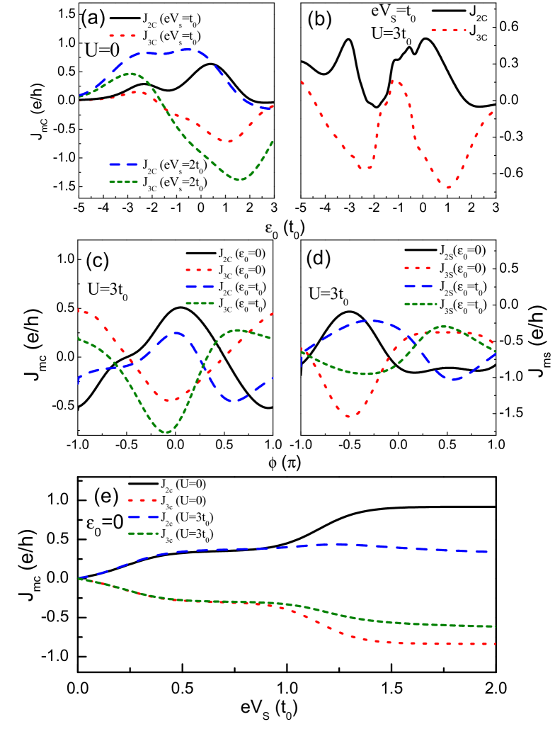
Figure 3: The current results in the cases of the finite spin bias. The temperature is assumed to be $k_{B}T=0.1t_{0}$. (a)-(b) The charge currents vs QD levels with $U=0$ and $U=3t_{0}$, respectively. (c)-(d) The charge and spin currents as functions of the magnetic flux. (e) The charge currents versus the spin bias strength.

It is evident that the above results are dependent on the electron transport properties in this structure. Then in order to clarify these results we focus on the transmission functions, as shown in Fig.2 with $\varepsilon_{j}=0$. They are just the integrands for the calculation of the charge currents [see Eq.(2)]. Here it is necessary to emphasize that although the Rashba-related spin-flip terms contribute to the electron transport, the spin-conserved electron motion determines the transport results of this system.gongapl So, to keep the argument simple, we drop the spin flip terms for the analysis of electron transport behaviors. By comparing the results shown in Fig.2(a), we can readily see that in the absence of magnetic flux, the traces of $T_{2\uparrow,1\uparrow}$ and $T_{3\downarrow,1\downarrow}$ coincide with each other very well, so do the curves of $T_{2\downarrow,1\downarrow}$ and $T_{3\uparrow,1\uparrow}$. Substituting this result into Eq.(10), one can certainly arrive at the result of the distinct charge currents in the drain terminals. On the other hand, these transmission functions depend nontrivially on the magnetic phase factor, as exhibited in Fig.2(b) with $\phi={\pi\over 2}$. In comparison with the zero magnetic field case, herein the spectra of $T_{j\downarrow,j^{\prime}\downarrow}$ are reversed about the axis $\omega=0$ without the change of their amplitudes, but the amplitudes of $T_{j\uparrow,j^{\prime}\uparrow}$ present a thorough change. Similarly, with the help of Eq.(10), one can then understand the disappearance of charge currents in such a case. Moreover, the presentation of spin currents can be understood with the help of above result and Eq.(11).

The underlying physics being responsible for the spin dependence of the transmission functions is quantum interference, which manifests if we analyze the electron transmission process in the language of Feynman path. Therefore based on this method, we write $T_{2\sigma,1\sigma}=|\tau_{2\sigma,1\sigma}|^{2}$ where the transmission probability amplitude is defined as $\tau_{2\sigma,1\sigma}=\widetilde{V}^{*}_{2\sigma}G^{r}_{2\sigma,1\sigma}\widetilde{V}_{1\sigma}$ with $\widetilde{V}_{j\sigma}=V_{j\sigma}\sqrt{2\pi\rho_{j}(\omega)}$. With the solution of $G^{r}_{2\sigma,1\sigma}$, we find that the transmission probability amplitude $\tau_{2\sigma,1\sigma}$ can be divided into three terms, i.e., $\tau_{2\sigma,1\sigma}=\tau^{(1)}_{2\sigma,1\sigma}+\tau^{(2)}_{2\sigma,1\sigma}$, where $\tau^{(1)}_{2\sigma,1\sigma}=\frac{1}{D}\widetilde{V}^{*}_{2\sigma}g_{2\sigma}t^{*}_{1\sigma}g_{1\sigma}\widetilde{V}_{1\sigma}$ and $\tau^{(2)}_{2\sigma,1\sigma}=\frac{1}{D}\widetilde{V}^{*}_{2\sigma}g_{2\sigma}t_{2\sigma}g_{3\sigma}t_{3}e^{i\phi}g_{1\sigma}\widetilde{V}_{1\sigma}$ with $D=\det\{[G^{r}]^{-1}\}\prod_{j}g_{j\sigma}$. By observing the structures of $\tau^{(1)}_{2\sigma,1\sigma}$ and $\tau^{(2)}_{2\sigma,1\sigma}$, we can readily find that they just represent the two paths from lead-2 to lead-1 via the QD ring. The phase difference between $\tau^{(1)}_{2\sigma,1\sigma}$ and $\tau^{(2)}_{2\sigma,1\sigma}$ is $\Delta\phi_{2\sigma}=[\phi-2\sigma\varphi+\theta_{3}]$ with $\theta_{j}$ arising from $g_{j\sigma}$. It is clearly known that only such a phase difference is related to the spin polarization. $T_{3\sigma,1\sigma}$ can be analyzed in a similar way. We then write $T_{3\sigma,1\sigma}=|\tau^{(1)}_{3\sigma,1\sigma}+\tau^{(2)}_{3\sigma,1\sigma}|^{2}$, with $\tau^{(1)}_{3\sigma,1\sigma}=\frac{1}{D}\widetilde{V}^{*}_{3\sigma}g_{3\sigma}t_{3}e^{i\phi}g_{1\sigma}\widetilde{V}_{1\sigma}$ and $\tau^{(2)}_{3\sigma,1\sigma}=\frac{1}{D}\widetilde{V}^{*}_{3\sigma}g_{3\sigma}t^{*}_{2\sigma}g_{2\sigma}t^{*}_{1\sigma}g_{1\sigma}\widetilde{V}_{1\sigma}$. The phase difference between $\tau^{(1)}_{4\sigma,1\sigma}$ and $\tau^{(2)}_{3\sigma,1\sigma}$ is $\Delta\phi_{3\sigma}=[\phi-2\sigma\varphi-\theta_{2}]$. Utilizing the parameter values in Fig.2, we evaluate that $\varphi\approx{\pi\over 7}$ and $\theta_{j}=-\frac{\pi}{2}$ at the point of $\omega=0$. It is apparent that when $\phi=0$ only the phase differences $\Delta\phi_{2\sigma}$ are spin-dependent. Accordingly, we obtain that $\Delta\phi_{2\uparrow}={-11\pi\over 14}$, $\Delta\phi_{2\downarrow}={3\pi\over 14}$, $\Delta\phi_{3\uparrow}={3\pi\over 14}$, and $\Delta\phi_{3\downarrow}={11\pi\over 14}$, which clearly prove that the quantum interference between $\tau^{(1)}_{2\uparrow,1\uparrow}$ and $\tau^{(2)}_{2\uparrow,1\uparrow}$ ($\tau^{(1)}_{3\downarrow,1\downarrow}$ and $\tau^{(2)}_{3\downarrow,1\downarrow}$ alike) is destructive, but the constructive quantum interference occurs between $\tau^{(1)}_{2\downarrow,1\downarrow}$ and $\tau^{(2)}_{2\downarrow,1\downarrow}$ ($\tau^{(1)}_{3\uparrow,1\uparrow}$ and $\tau^{(2)}_{3\uparrow,1\uparrow}$ alike). Then such a quantum interference pattern can explain the traces of the transmission functions shown in Fig.2(a). In the case of $\phi=\frac{\pi}{2}$ we find that only $\Delta\phi_{2(3)\sigma}$ are crucial for the occurrence of spin polarization. By a calculation, we obtain $\Delta\phi_{2\uparrow}=-{2\pi\over 7}$, $\Delta\phi_{2\downarrow}={2\pi\over 7}$, $\Delta\phi_{3\uparrow}={5\pi\over 7}$, and $\Delta\phi_{3\downarrow}={9\pi\over 7}$, which are able to help us clarify the results in Fig.2(c) and (d). Up to now, the characteristics of the transmission functions, as shown in Fig.2, hence, the tunability of charge currents have been clearly explained by analyzing the quantum interference between the transmission paths.

For the case of finite spin bias, the charge currents in lead-2 and lead-3 can be evaluated by Eq.(2). Accordingly, in Fig.3(a)-(b) we plot the charge current spectra vs the QD levels. In Fig.3(a), we find that different from the linear transport results, the current spectra exhibit complicated properties with the shift of QD levels, since the currents are not proportional to the transmission function any more. For the case of $eV_{s}=t_{0}$, the quantitative relation between these two charge currents ( i.e., $J_{2c}=-J_{3c}$) is seeable ( only in the region of $\varepsilon_{0}$ greater than $-t_{0}$ and less than $t_{0}$ ). When the spin-bias strength is increased to $eV_{s}=2t_{0}$, the magnitude of the charge currents increase. Meanwhile, it is seen that the curve of $J_{2c}$ tends to be symmetric and the profile of $J_{3c}$ becomes asymmetric. Consequently, here the relation of $J_{2c}=-J_{3c}$ becomes ambiguous except at the position of $\varepsilon_{0}=0$.

By far, we have not discussed the effect of electron interaction on the occurrence of charge currents in the drain terminals, though it is included in our theoretical treatment. Now we incorporate the electron interaction into the calculation with $U_{j}=U=3t_{0}$, and we deal with the many-body terms by employing the second-order approximation, since such an approximation is feasible for the case the system temperature higher than the Kondo temperature (where the electron correlation is comparatively weak). Fig.3(b) shows the calculated currents spectra vs the QD levels with $k_{B}T=0.1t_{0}$. From this figure, we see that the many-body effect causes the further oscillation of the charge current spectra. It is obvious that the intradot electron interaction splits the current curves into two groups, and in each group the current properties are analogous to those in the noninteracting case. This is because that within such an approximation the Coulomb interaction only gives rise to the splitting of the QD level, i.e., $\varepsilon_{j}$ and $\varepsilon_{j}+U$. As a result, one can find in such a case, in the high-energy and low-energy regimes (i.e., around the points of $\varepsilon_{0}=0$ and $\varepsilon_{0}=-3t_{0}$) the result of $J_{2c}=-J_{3c}$ is also seeable. On the other hand, it shows that the effect of the Coulomb interaction on the spin currents is nontrivial, and in the region of $0<\phi<\pi$ the magnitudes of the spin currents are suppressed [see Fig.3(d)].

Finally, we investigate the charge currents as functions of the spin-bias strength, with the calculated results shown in Fig.3(e). First, at the noninteracting case, we see that in the situation of $0<eV_{s}<{t_{0}\over 2}$ (or $t_{0}<eV_{s}<{3t_{0}\over 2}$), the charge currents increase with the strengthening of spin bias. But next when the spin bias strength varies in the regime of ${t_{0}\over 2}<eV_{s}<t_{0}$ (or ${3t_{0}\over 2}<eV_{s}<2t_{0}$), the magnitudes of the charge currents change a little. However, when the many-body effect is taken into account, it is found that only in the situation of $0<eV_{s}<{t_{0}\over 2}$, the magnitudes of the charge currents are proportional to the strengthening of spin bias, whereas in the cases the charge currents are approximately independent of the variation of the spin bias.

IV Summary

In summary, in the present triple-QD ring, the local Rashba interaction provides a spin-dependent AB phase difference. The three-terminal configuration balances the electron transmission probabilities via two different arms of the QD ring. The variation of the magnetic field strength and the QD level can adjust the phase difference between the two kinds of Feynman paths on an equal footing. Thus, the spin dependence of the electron transmission probability can be controlled by altering the exerted magnetic field or the QD levels. Then with the consideration of a spin bias in one terminal, it is possible to obtain the tunable charge and spin currents in the either two terminals. On the other hand, we readily emphasize that when the spin bias is considered in another terminal(e.g., lead-2), the direction of the charge current in lead-3 will be inverted since the geometry of this structure. However, if the Rashba interaction is applied in another QD (e.g., QD-2) we can also see the inversion of the current directions in lead-3. That is to say, the current directions in either drain terminal can be modulated by controlling the spin bias or Rashba interaction. So, such a structure can be proposed to be a prototype of a charge and spin current rectifier.

References

- (1) Y. Ohno, D. K. Young, B. Beschoten, , Nature, 402 (1999) 790.
- (2) Zutic, J. Fabian, and S. Das Sarma, Rev. Mod. Phys. 76 (2004) 323; R. Hanson, L. P. Kouwenhoven, J. R. Petta, S. Tarucha, and L. M. K. Vandersypen, Rev. Mod. Phys. 79 (2004) 1217; S. A. Wolf, ., Science 294 (2001) 1488.
- (3) D. Loss, and D. P. DiVincenzo, Phys. Rev. A 57 (1998) 120; G. Burkard, D. Loss, and D. P. DiVincenzo, Phys. Rev. B 63 (1999) 2070.
- (4) D. V. Bulaev and D. Loss, Phys. Rev. B 71 (2005) 205324.
- (5) A. A. Kiselev and K. W. Kim, Appl. Phys. Lett. 78 (2001) 775; T. P. Pareek, Phys. Rev. Lett. 92 (2004) 076601.
- (6) J. Nitta, T. Akazaki, H. Takayanagi, and T. Enoki, Phys. Rev. Lett. 78 (1997) 1335.
- (7) G. Engels, J. Lange, Th. Schäpers, and H. Lüth, Phys. Rev. B 55, R1958 (1997); D. Grundler, Phys. Rev. Lett. 84 (2000) 6074.
- (8) Q. F. Sun, J. Wang, and H. Guo, Phys. Rev. B 71 (2005) 165310; B. K. Nikolic and S. Souma, Phys. Rev. B 71 (2005) 195328.
- (9) P. Trocha and J. Barnas, Phys. Rev. B 76 (2007) 165432; P. Trocha and J. Barnas, Phys.: Condens. Matter 20 (2008) 125220.
- (10) M. L. Ladrón de Guevara and P. A. Orellana , Phys. Rev. B 73, (2006) 205303.
- (11) A. Brataas, Y. Tserkovnyak, G. E. W. Bauer and B. I. Halperin, Phys. Rev. B 66 (2002) 060404; S. O. Valenzuela and M. Tinkham, Nature (London) 442 (2006) 176; Y. K. Kato, R. C. Myers, A. C. Gossard and D. D. Awschalom, Science 306 (2004) 1910; S. D. Ganichev, et al., Nature Physics 2 (2006) 609.
- (12) J. Hubner, et al., Phys. Rev. Lett., 90 (2003) 216601; Martin J. Stevens et al., Phys. Rev. Lett, 90 (2003) 136603.
- (13) M. Y. Veillette, C. Bena, and L. Balents, Phys. Rev. B 69 (2004) 075319; X.-D. Cui, S.-Q. Shen, J. Li, Y. Ji, W. Ge, and F.-C. Zhang, Appl. Phys. Lett. 90 (2007) 242115.
- (14) J. Li and S. Q. Shen, Phys. Rev. B 76 (2007) 153302; P. Zhang, Q. K. Xue, and X. C. Xie, Phys. Rev. Lett. 91 (2003) 196602.
- (15) H. Katsura,J. Phys. Soc. Jpn. 76 (2007) 054710; Y.-J. Bao, N.-H. Tong, Q.-F. Sun, and S.-Q. Shen, Europhys. Lett. 83 (2008) 37007.
- (16) H.-Z. Lu and S.-Q. Shen, Phys. Rev. B 77 (2008) 235309; H.-Z. Lu, B. Zhou, and S.-Q. Shen, Phys. Rev. B 79 (2009) 174419; H.-Z. Lu and S.-Q. Shen, Phys. Rev. B 80 (2009) 094401.
- (17) F. Chi, and X. Q. Yuan, Chi. Phys. Lett. 26,(2009) 097301.
- (18) K. Bao and Y. Zheng, Phys. Rev. B 73 (2006) 045316.
- (19) S. Amaha, T. Hatano, T. Kubo, S. Teraoka, Y. Tokura, S. Tarucha, and D. G. Austing, Appl. Phys. Lett. 94 (2009) 092103.
- (20) W. Gong, Y. Zheng, and T. Lü, Appl. Phys. Lett. 92, 042104 (2008); W. Gong, Y. Han, and G. Wei, Sol. Stat. Comm. 149, 1831(2009).
- (21) D. Sànchez and L. Serra, Phys. Rev. B 74, 153313 (2006).
- (22) Y. Meir and N. S. Wingreen, Phys. Rev. Lett. 68, 2512 (1992); A.-P. Jauho, N. S. Wingreen, and Y. Meir, Phys. Rev. B 50, 5528 (1994).
- (23) W. Gong, Y. Zheng, Y. Liu, and T. Lü, Phys. Rev. B 73 (2006) 245329.
- (24) J. Q. You and H. Z. Zheng, Phys. Rev. B 60 (1999) 13314; J. Q. You and H. Z. Zheng, Phys. Rev. B 60 (1999) 8727.
- (25) J. Nitta, T. Akazaki, H. Takayanagi, and T. Enoki, Phys. Rev. Lett. 78, 1335 (1997); F. Mireles and G. Kirczenow, Phys. Rev. B 64, 024426 (2001).
- (26) A. M. Lobos and A. A. Aligia, Phys. Rev. Lett. 100, 016803 (2008); R. J. Heary, J. E. Han, and Lingyin Zhu Phys. Rev. B 77, 115132 (2008); R. Citro, and F. Romeo, Phys. Rev. B 77, 193309 (2008).