Model-independent X-ray mass determinations

Abstract

A new method is introduced for making X-ray mass determinations of spherical clusters of galaxies. Treating the distribution of gravitating matter as piecewise constant and the cluster atmosphere as piecewise isothermal, X-ray spectra of a hydrostatic atmosphere are determined up to a single overall normalizing factor. In contrast to more conventional approaches, this method relies on the minimum of assumptions, apart from the conditions of hydrostatic equilibrium and spherical symmetry. The method has been implemented as an xspec mixing model called clmass, which was used to determine masses for a sample of nine relaxed X-ray clusters. Compared to conventional mass determinations, clmass provides weak constraints on values of $M_{500}$, reflecting the quality of current X-ray data for cluster regions beyond $r_{500}$. At smaller radii, where there are high quality X-ray spectra inside and outside the radius of interest to constrain the mass, clmass gives confidence ranges for $M_{2500}$ that are only moderately less restrictive than those from more familiar mass determination methods. The clmass model provides some advantages over other methods and should prove useful for mass determinations in regions where there are high quality X-ray data.

1. Introduction

The need for accurate masses for galaxy clusters is motivated by more than their significance as fundamental parameters of the most massive, dynamically stable structures in the universe. Because gravity is dominant on the largest scales in the universe, masses of the largest virialized structures are important cosmological probes (e.g. Voit, 2005; Allen et al., 2008; Samushia & Ratra, 2009). For example, the growth of structure at high mass scales provides a sensitive means to measure the power spectrum of density fluctuations that emerged from the early universe and to determine the time dependence of the rate of cosmic expansion, hence placing useful constraints on cosmological models (Vikhlinin et al., 2009b).

The dominance of gravity in clusters also means that there are several avenues for clusters mass determinations, which can be classified broadly as dynamical (e.g. Girardi et al., 1998; Rines et al., 2003), gas dynamical (e.g. Pointecouteau et al., 2005; Vikhlinin et al., 2006) and lensing (e.g. Smith et al., 2005; Limousin et al., 2007). No approach is free of weaknesses. Dynamical mass determinations are limited by our inability to measure velocities transverse to the line-of-sight (e.g. Mamon & Boué, 2009). Gas dynamical methods rely on the intracluster medium (ICM) being hydrostatic (cf. Markevitch & Vikhlinin, 2007) and they require accurate determinations of the total pressure of the ICM (e.g. Churazov et al., 2008; Mahdavi et al., 2008). Strong lensing is confined to the highest density regions of rich clusters (e.g. Newman et al., 2009), while weak lensing is affected by substantial statistical uncertainties for individual clusters, line-of-sight projections and the mass-sheet degeneracy (e.g. Metzler et al., 2001; Hoekstra, 2003; Bradač et al., 2004; Zhang et al., 2008). Many of these issues can be addressed by judicious choice of targets, but the most reliable results are likely to come from the application of multiple mass determination methods to cross check and augment one another (e.g. Mahdavi et al., 2007; Churazov et al., 2008; Newman et al., 2009).

This paper introduces a new approach to X-ray mass determinations. The method relies on the same basic assumptions as other X-ray mass determinations, i.e., that the intracluster gas is hydrostatic and spherically symmetric. However, it largely avoids the additional, model-dependent assumptions that are required by other approaches. The method is outlined in section 2 and applied to a sample of clusters with high quality Chandra data in section 3. Strengths and weaknesses of the method are related to the results in section 4.

Following Vikhlinin et al. (2006), all distances are computed assuming a flat $\Lambda$CDM cosmology, with $\Omega_{\rm M}=0.3$ and a Hubble constant of $72\rm\ km\ s^{-1}\ Mpc^{-1}$. For each cluster, the radii $r_{500}$ and $r_{2500}$ enclose regions with densities of 500 and 2500, respectively, times the critical density at the cluster redshift, while $M_{500}$ and $M_{2500}$ are the corresponding enclosed masses. Confidence ranges are determined at the 90% level except where stated otherwise.

2. Method

X-ray mass determinations rely on the ability of X-ray observations to determine the temperature and density of the hot ICM. In an ICM dominated by hot gas, the pressure is determined by its temperature and density. Undetected components of the ICM, i.e., nonthermal particles, magnetic fields and turbulence, can add to the effective pressure, although simulations (e.g. Nagai et al., 2007) and observations (e.g. Churazov et al., 2008) suggest that these contributions are modest, of the order of $10\%$, in relaxed appearing clusters. Since the purpose of this paper is to introduce a new approach to X-ray mass determinations, such effects are not considered further here, but they need to be understood for precise mass determinations.

If the gravitational potential is spherically symmetric and the ICM is in hydrostatic equilibrium, the distribution of the ICM is governed by the equation of hydrostatic equilibrium,

$${dp\over dr}=-\rho_{\rm g}(r){GM(r)\over r^{2}},$$ (1)

where $p(r)$ is the gas pressure, $\rho_{\rm g}(r)$ is its density and $M(r)$ is the total gravitating mass within the radius, $r$. If the pressure and density distributions of the ICM are known, $M(r)$ can be determined from this equation. In practice, properties of the ICM (particularly its temperature) are only determined at discrete radii, so that the pressure derivative is constrained poorly, if at all, by the data. With few exceptions (Nulsen & Bohringer, 1995; Arabadjis et al., 2004), mass determinations circumvent this difficulty by employing model-dependent assumptions to supplement equation (1). Details vary widely, but typical approaches assume analytic forms, with a modest number of parameters, either for the mass profile (e.g. Mahdavi et al., 2007), or for the temperature and density profiles (e.g. Vikhlinin et al., 2006). For example, using the latter approach, substituting the analytic form for the pressure and density profiles in equation (1) gives an analytic expression for $(1/\rho_{\rm g})dp/dr$, with parameters that can be determined by fitting the analytic temperature and density profiles to the discrete temperatures and densities obtained from X-ray spectra.

Also with few exceptions (e.g. Mahdavi et al., 2007), several steps are required to obtain a cluster mass, so that a confidence range for the mass is determined indirectly from fitting the X-ray spectra. For example, data may be “deprojected” to obtain gas temperatures and densities (with strongly correlated errors). Deprojected temperatures and densities are then fitted with analytic models to determine their parameters, which are used to obtain the mass, as described above. Doing mass determinations in several steps simplifies the overall process, but it complicates error determinations, since errors must be propagated through all steps. While there are well-known statistical methods for computing confidence ranges in such cases, the many parameters involved (at the very least, one temperature and one density for each X-ray spectrum), make the process cumbersome and expensive. Error propagation is more flexible when it is possible to marginalize over fitting parameters directly to compute a confidence range for the mass. This is considerably easier when the mass can be determined directly in terms of parameters used to fit to the X-ray data, as in the approach used here.

2.1. A model-independent approach

A simple model can be used to approximate any spherical cluster and its atmosphere well. The cluster volume is divided into a series of spherical shells centered on the cluster and, in addition to the assumptions of spherical symmetry and hydrostatic equilibrium, it is assumed that

• the gravitating matter density in each spherical shell is constant and

• the gas in each spherical shell is isothermal.

Assuming that the gravitating matter density is constant in shells provides, essentially, the simplest continuous mass distribution that is nonsingular at $r=0$, which can approximate any real mass distribution well with a large number of shells. Similarly, assuming that the shells are isothermal results in, perhaps, the simplest gas model that can approximate any real, spherically symmetric, gas temperature distribution well with a large enough number of shells. Projected onto the sky, the spectrum for any region of the model cluster is a sum of optically thin, thermal models, a form that can be expressed conveniently as an xspec mixing model (Arnaud, 1996).

Although the term is inappropriate in the strict mathematical sense, since this model can approximate arbitrary mass and temperature distributions, we call the method “model-independent.” The model used here is one instance of a broad class of (model-independent and model-dependent) approximations that could be used for the gravitating matter distribution (alternative models would differ in equations 2 and 3 below).

Denoting radii measured from the center of the cluster by $r$ and the shell boundaries by $r_{1},r_{2},\ldots,r_{n+1}$ in increasing order, the $i^{\rm th}$ shell is the region with $r_{i}<r<r_{i+1}$. If the gravitating matter density within the $i^{\rm th}$ shell is $\rho_{i}$, then the gravitating mass distribution within the shell is given by

$$M(r)=M_{i}+{4\pi\over 3}\rho_{i}(r^{3}-r_{i}^{3}),$$ (2)

where $M_{i}=M(r_{i})$ is the total gravitating mass within $r_{i}$. The gravitational potential within the $i^{\rm th}$ shell is then given by

$$\Phi(r)-\Phi(r_{i})=\int_{r_{i}}^{r}{GM(r)\over r^{2}}\,dr=\left[{GM_{i}\over r_{i}}+{2\pi\over 3}G\rho_{i}(r-r_{i})(r+2r_{i})\right]{r-r_{i}\over r}.$$ (3)

Since the gas in each shell is assumed to be isothermal and hydrostatic, within the $i^{\rm th}$ shell the electron density can be expressed as

$$n_{{\rm e}}(r)=n_{{\rm e},i}\exp\left[-{\mu m_{\rm H}\{\Phi(r)-\Phi(r_{i})\}\over kT_{i}}\right],\qquad{\rm for}\ r_{i}<r<r_{i+1},$$ (4)

where $n_{{\rm e},i}$ is the electron density at the inner edge of the $i^{\rm th}$ shell, $T_{i}$ is the gas temperature in that shell, $\Phi(r)$ is the gravitational potential, $k$ is Boltzmann’s constant and $\mu m_{\rm H}$ is the mean mass per particle in the gas. For the gas to be hydrostatic, the pressure must be continuous from shell to shell, but, as the temperature is generally discontinuous at shell boundaries, so is the gas density. Pressure continuity between shells $i$ and $i+1$ requires

$$n_{{\rm e},i+1}T_{i+1}=n_{{\rm e},i}\exp\left[-{\mu m_{\rm H}\{\Phi(r_{i+1})-\Phi(r_{i})\}\over kT_{i}}\right]T_{i},$$ (5)

which determines $n_{{\rm e},i+1}$ in terms of $n_{{\rm e},i}$, the temperatures and the potential.

Together, these results show that when the gravitating matter density and gas temperature are specified for each shell, under the model assumptions, the gas density is determined throughout the model atmosphere, up to a single scale factor that may be regarded as the electron density, $n_{{\rm e},1}$, at the inner edge of the innermost shell (usually $r=0$).

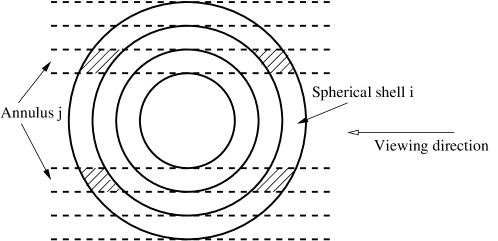
Figure 1.— Shells and annuli used for the mass model. This schematic shows a cross-section through a cluster center that contains our line-of-sight. Dashed lines show boundaries of cylindrical regions that project onto the annuli on the sky from which X-ray spectra are extracted. Full lines show boundaries of the corresponding spherical shells.

When observing a spherical cluster, the normal practice is to divide the sky into concentric annuli centered on the cluster and extract a spectrum from each annulus. An annulus is the projection onto the sky of a cylindrical region in the cluster. The schematic in Fig. 1 shows sections through some cylinders (bounded by dashed lines) in a plane that contains our line-of-sight through the cluster center, i.e., the common axis of the cylinders. We now define the spherical shells discussed above to have radial bounds matching those of the cylinders (full lines in Fig. 1). Denoting cylindrical radii, measured from the line-of-sight through the center of the cluster, by $\varpi$, the $j^{\rm th}$ cylindrical region is then defined by $\varpi_{j}\leq\varpi\leq\varpi_{j+1}$ and, by construction, $r_{i}=\varpi_{i}$, which simplifies some of the following results. The same geometric arrangement is used for deprojections.

To complete the spectral model, we need to calculate the emission measure of the gas from the $i^{\rm th}$ shell that appears in the $j^{\rm th}$ annulus, i.e., the emission measure of the gas in the intersection between the $i^{\rm th}$ shell and the $j^{\rm th}$ cylinder (hatched region in Fig. 1),

$${\rm EM}_{{i},{j}}=\int_{\rm Intersection}n_{{\rm e}}n_{\rm H}\,dV=4\pi\int_{r_{i}}^{r_{i+1}}n_{{\rm e}}(r)n_{\rm H}(r)\left(\sqrt{r^{2}-r_{j}^{2}}-\sqrt{r^{2}-r_{j+1}^{2}}\right)r\,dr,$$ (6)

where each square root should be taken as zero if its argument is negative. These integrations are carried out numerically. Note that for $i<j$, since the $i^{\rm th}$ spherical shell does not intersect the $j^{\rm th}$ cylinder, ${\rm EM}_{{i},{j}}=0$. The model spectrum for the $j^{\rm th}$ annulus is given as a sum over the shells of the thermal model for each spherical shell, weighted by its emission measure in the $j^{\rm th}$ cylinder, i.e., the spectrum is

$$F_{j}(E)=\sum_{i=j}^{n}{\rm EM}_{{i},{j}}f(E,T_{i},A_{i}),$$ (7)

where $f(E,T_{i},A_{i})$ is the thermal spectrum for the $i^{\rm th}$ spherical shell (for unit emission measure). The parameter, $A_{i}$, is a placeholder for all thermal model parameters, including abundances, apart from the temperature.

High quality spectra are required to obtain good results when fitting this model. Since the demands of the model are similar to those of deprojections, it is expected that the minimum required source count per spectrum is several thousand. There is a clear trade off between reducing shell width to gain spatial resolution and increasing it to improve spectral signal-to-noise (see section 4.2).

2.2. Implementation

The model outlined above has been implemented as an xspec mixing model called clmass. This mixing model has two parameters per spherical shell, the gas temperature and the gravitating matter density. The temperature for each shell must be linked (equated) to the temperature parameter of a thermal model for that shell. As noted, there is a single overall gas density scale that is free in the model. For the mixing model, it is convenient to make the xspec norm for the innermost shell the free parameter instead of the central gas density, $n_{{\rm e},1}$. The xspec norm is the emission measure multiplied by a scale factor that is the same for each shell and depends on the distance to a cluster. In using the clmass model, the xspec norm for every outer shell is linked (equated) to that of the central shell and the X-ray flux for the $i^{\rm th}$ annulus (equation 7) is given by

$$S_{j}(E)=K\sum_{i=j}^{n}W_{i,j}f(E,T_{i},A_{i}),$$ (8)

where $K$ is the single free norm (for the innermost shell) and there are $n$ spherical shells. The weights, $W_{i,j}={\rm EM}_{{i},{j}}/{\rm EM}_{{1},{1}}$, are completely determined by the parameters of the mixing model.

Frequently, a cluster extends beyond the field of view of an X-ray detector, so that there is X-ray emission in the field of view originating from gas lying beyond the outer edge of the outermost spherical shell (the $n^{\rm th}$ shell) of the clmass model. There is no entirely satisfactory way to deal with such emission, but we often want to use such nonideal data for mass determinations. Using a local X-ray background measured immediately outside the $n^{\rm th}$ annulus generally overestimates the “background” gas emission in all inner shells. Based on empirical fits to gas density profiles, the clmass model allows the alternative of assuming that the gas density profile beyond the inner edge of the $n^{\rm th}$ shell follows a beta model,

$$n_{{\rm e}}(r)=n_{{\rm e},0}(1+r^{2}/a^{2})^{-3\beta/2},$$ (9)

where $\beta$ and $a$ are constant parameters. The gas density at the inner edge of the $n^{\rm th}$ shell is still determined by pressure continuity (equation 5), but, instead of using the gas density profile from equation (4), the emission measure for the $n^{\rm th}$ shell in each annulus is determined by integrating the beta model to infinity along our line-of-sight (giving results in terms of incomplete beta functions). Together with a switch that determines whether or not this feature is used, the beta model adds three fixed parameters to the clmass model. This feature is at odds with the model-independent approach of clmass otherwise. Ideally, it should be avoided by using X-ray data that cover the whole of a cluster.

For the sake of brevity, the new mass model will be referred to as clmass in the remaining discussion. Much of that discussion would apply to any implementation of the model, although there are some comments on limitations that are specific to the xspec implementation, as noted.

3. Masses for a sample of galaxy clusters

3.1. Sample and data preparation

The clmass model has been applied to Chandra data for a subsample of the clusters analyzed by Vikhlinin et al. (2006) and Vikhlinin et al. (2009a). Target clusters were chosen to sample a broad range of cluster temperatures, hence masses. Clusters analyzed here are listed with some of their basic properties in Table 1.

Table 1The cluster sample

Cluster	z	$r_{2500}$	$r_{500}$	Chandra ObsID
		(kpc)	(kpc)
A907	0.1603	501	1095	3185, 3205, 535
A1413	0.1429	559	1300	1661, 5002, 5003
A1991	0.0592	341	734	3193
A2029	0.0779	642	1359	891, 4977, 6101
A2390	0.2302	561	1414	4193
A1835	0.2520	673	1475	6880, 6881, 7370
A1650	0.0845	515	1128	5822, 5823, 6356, 6357, 6358, 7242
A3112	0.0761	459	1025	2216, 2516, 6972, 7323, 7324
A2107	0.0418	416	919	4960

To simplify comparison with the results of Vikhlinin et al., our analysis parallels theirs closely, using the same X-ray spectra as far as possible with the clmass model. Details of the spectral reductions can be found in Vikhlinin et al. (2005). The spectra were extracted from annuli with radial bounds having $\varpi_{j+1}=1.5\varpi_{j}$, for $j>1$. Since the gravitating matter density is constant in the corresponding spherical shells, the matter density profile is sampled rather coarsely in the resulting model. To make our masses directly comparable, we have also adopted the values of $r_{2500}$ and $r_{500}$ from Vikhlinin et al. (Table 1). Note that this eliminates a source of uncertainty in $M_{2500}$ and $M_{500}$, reducing confidence ranges compared to ab initio determinations of these masses.

Vikhlinin et al. combined spectra from the different front illuminated (FI) chips into single spectra. However, because they have significantly different responses, FI spectra were kept separate from those extracted from the back illuminated (BI) chips. This means that the number of spectra per annulus for a cluster can vary in the transition regions between FI and BI chips. The version of clmass used here inherited from projct a requirement that the same number of spectra be used for every data group. Particularly for observations with ACIS-S at the aim point, this means that we were unable to use every available spectrum for some annuli. In cases where a choice had to be made, we opted for the spectrum with the greater source count. As a result, we used slightly fewer spectra than Vikhlinin et al. for some mass determinations. This shortcoming of clmass will be remedied in a future version.

A limitation of xspec mixing models is that they must be applied after all other model components. This is inconvenient for several reasons. Photoelectric absorption due to foreground gas should be applied to the spectrum emerging from each annulus, after it is emitted by a cluster. In practice, the foreground absorption usually does not vary significantly across a cluster, so that it is satisfactory to apply the same absorption model to each thermal model before the mixing model. However, there are clusters where the absorbing column varies significantly, which cannot be modeled well by the clmass model in xspec.

Another inconvenience arises in background corrections. In the standard approach, background spectra are constructed from source free exposures, processed and scaled to match the observations. Variations of the particle background and the soft X-ray background with time and position can leave residual backgrounds requiring further correction. These are often addressed by model components added to the annular spectra (Vikhlinin et al., 2005), but this approach cannot be used in conjunction with an xspec mixing model. Here, the residual backgrounds are corrected using a specially prepared corrfile for each annular spectrum. Depending on need, one or two soft thermal components were fitted to the spectrum from the outermost annulus for each cluster (to account for a residual soft background and any emission from the North Polar Spur). These components were scaled by area and added to the existing corrfile for each annulus (already employed to correct for the read out artifact; Vikhlinin et al., 2005).

Gratifyingly, inclusion of the beta model feature described in section 2.2 had little effect on the quality of the model fits and on the masses. This is to be expected, since the clusters are barely detected in the largest annuli, so there should be little need to account for cluster emission from regions beyond the outermost shells.

3.2. Cluster Masses

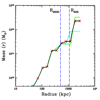
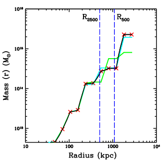
Figure 2.— Mass profiles for Abell 907. The black line shows the cumulative mass distribution for the best fitting clmass model when no constraints are applied to the gravitating matter densities. Crosses mark the shell boundaries. Large variations in slope from shell-to-shell reflect large variations in the gravitating matter density. Left panel: The cyan line shows the mass profile at the upper 90% confidence limit for the mass within $r_{500}$, i.e., $M_{500}$, and the green line shows the corresponding mass profile at the lower 90% confidence limit. Right panel: Same for $M_{2500}$.

The clmass mixing model was combined with an absorbed thermal model, $\textsc{wabs}{}*\textsc{mekal}$, to fit the sample clusters. Column densities for photoelectric absorption were set to the values used by Vikhlinin et al. (2005). As discussed in section 2.2, many parameters must be linked to use the clmass model. Since the number of shells provided by the model is fixed, usually there are unused parameters that must also be frozen. Parameters were given reasonable initial values to forestall numerical problems (section 2.2). With $\sim 10$ annuli per cluster, in order to avoid error prone manipulations of numerous parameters, these steps were automated in xspec Tcl scripts. Abundances were generally free in the fits, but where they were poorly constrained or took on unreasonable values, abundances for groups of adjacent shells were tied together to produce physically reasonable results. Since they have little impact on the masses, we do not consider abundances further. All free parameters and links used for the fits were maintained when determining confidence ranges for the masses.

Initial attempts to fit the data showed that the clmass model does not generally constrain the gravitating matter density tightly for individual shells. This is because the gravitational potential is governed by the accumulated mass within any radius and variations of the gas density depend on changes in the potential. Since there are two integrations between the mass density and changes in the potential, the gas density, hence the spectra, are only affected at second order by local changes in the gravitating matter density (equation 3). Splitting the gravitating matter from one shell into the two adjacent shells, in suitable proportions, has little impact on the fit. In the presence of noise, this freedom to exchange mass from shell to shell results in large shell to shell variations of gravitating mass density, producing noisy best fitting mass profiles like that for Abell 907 in Fig. 2.

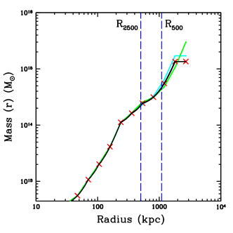
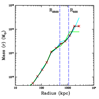
Figure 3.— Mass profiles for Abell 907 with the gravitating matter density constrained to be monotonic. Details as in Fig. 2.

The freedom of gravitating mass to shift between adjacent shells can be limited to some extent by constraining the gravitating matter density to be a monotonically decreasing function of the radius. This constraint improves model behaviour with a relatively minor impact on the goodness of fit (Table 2). In practice, the constraint requires gravitating mass densities to be linked for groups of adjacent shells where the unconstrained density would otherwise increase with radius. Mass profiles for Abell 907, with the gravitating matter density forced to be monotonic, are shown in Fig. 3. Evidently, the monotonic constraint makes the matter density profile considerably smoother. Although this condition is not required of the gravitating matter density distribution, it is simple, physically reasonably and relatively weak, while it reduces the noise in the mass profiles significantly. As a consequence, we prefer results for “monotonic” mass profiles in the following, although some results for unconstrained mass profiles are also given for comparison.

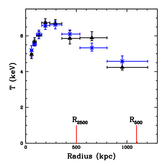
Figure 4.— Temperature profiles for Abell 907. Black triangles show temperatures for the best fitting “monotonic” clmass model. Blue crosses show the (projected) temperature profile of Vikhlinin et al. (2005). Temperature errors are 68% confidence ranges for individual shells. Radial error bars show extents of the annuli. clmass temperatures are deprojected, which generally makes them noisier than projected temperatures.

Once the temperatures have been determined, gas densities are governed by the distribution of gravitating matter. Loosely speaking, when fitting the clmass model, temperatures are determined by spectral shapes, so that the gravitating matter densities are determined by the radial distribution of the X-ray emission (i.e., emission measure). However, this is only a rule of thumb. Especially in the outskirts of clusters where the X-ray emission is not well detected above the background, fitted temperatures may be poorly constrained by the spectra, so that the temperatures can also respond to variations in X-ray brightness. This may result in large temperature excursions in response to poorly modeled fluctuations in X-ray brightness. Also, since the temperatures apply to gas in the spherical shells, they are deprojected temperatures. Like other deprojected temperatures, the spectral models are coupled from shell-to-shell, making the temperatures etc., prone to fluctuate from shell-to-shell. This effect can be seen in Fig. 4, which compares the best fitting clmass temperature profile for Abell 907 to the projected temperature profile of Vikhlinin et al. (2005).

Table 2Cluster masses

	Unconstrained		Monotonic
Cluster	$\chi^{2}/\rm dof$	$M_{500}$	$\chi^{2}/\rm dof$	$M_{500}$	$M_{2500}$
		($10^{14}\ M_{\odot}$)		($10^{14}\ M_{\odot}$)	($10^{14}\ M_{\odot}$)
A907	$692.4/626$	$3.2_{-0.7}^{+3.2}$	$693.7/630$	$4.7_{-0.5}^{+0.6}$	$2.2_{-0.3}^{+0.4}$
A2390	$840.9/626$	$23.0_{-14.8}^{+13.3}$	$846.2/632$	$14.9_{-5.3}^{+9.1}$	$4.0_{-1.1}^{+0.5}$
A1835	$489.4/290$	$7.1_{-1.3}^{+17.4}$	$491.7/293$	$7.1_{-1.3}^{+12.0}$	$7.1_{-2.1}^{+1.0}$
A1650	$669.1/301$	$5.1_{-1.5}^{+7.1}$	$673.2/306$	$5.8_{-1.3}^{+3.9}$	$2.1_{-0.2}^{+0.2}$
A3112	$545.8/314$	$3.0_{-1.1}^{+4.4}$	$546.7/317$	$2.8_{-0.9}^{+2.4}$	$1.7_{-0.3}^{+0.3}$
A2029	$2988.0/664$	$6.6_{-1.5}^{+4.5}$	$2993.5/669$	$7.1_{-1.8}^{+4.0}$	$5.0_{-0.6}^{+0.3}$
A1991			$563.7/326$	$5.9_{-4.0}^{+4.6}$	$0.8_{-0.2}^{+0.4}$
A1413	$449.0/313$	$7.9_{-3.9}^{+10.5}$	$450.3/321$	$9.1_{-3.2}^{+5.9}$	$3.6_{-0.6}^{+0.5}$
A2107			$428.1/299$		$1.3_{-0.3}^{+0.3}$

Cluster masses obtained from the clmass model are given in Table 2. Consistent with the model assumptions, gravitating matter densities are treated as constant within each shell, so that mass profile within a shell is as given by equation (2). Best fitting chi squareds for the unconstrained fits are given in column 2 and the corresponding values of $M_{500}$ are in column 3. The best fitting chi squareds for the monotonic fits are in column 4, with corresponding values of $M_{500}$ and $M_{2500}$ in columns 5 and 6, respectively. Values used for $r_{500}$ and $r_{2500}$ are given in Table 1. There are no results for $M_{500}$ for Abell 2107 because the Chandra data for it do not reach $r_{500}$. No unconstrained result is given for Abell 1991, the coolest and faintest cluster in the sample, because the unconstrained clmass model places no useful 90% upper limit on $M_{500}$ for it. Abell 1991 is not detected at high significance in annuli beyond $r_{500}$, so that the emission measures of the corresponding shells can be made arbitrarily small in the models. This permits an arbitrarily large gravitating mass in the shell immediately inside $r_{500}$. Making the gravitating matter density monotonic prohibits the density in the outermost shell within $r_{500}$ from exceeding that in the next inner shell, so that the mass of Abell 1991 can no longer be arbitrarily large. Thus we do get a confidence range for $M_{500}$ using the constrained clmass model.

Based on chi squared, all of the fits are formally unacceptable. However, all clusters show some departures from spherical symmetry and many also show evidence of ongoing minor merger activity (e.g. Markevitch & Vikhlinin, 2007), so that we should expect modest departures from hydrostatic equilibrium too. Considered in this light, it is gratifying that the coarsely resolved clmass model used here gives reduced chi squareds of less than 2 in most cases. The clear exception is Abell 2029, with reduced chi squareds of $\simeq 4.5$. Abell 2029 is the only cluster in the sample for which there are both ACIS-I and ACIS-S observations, giving two complete sets of spectra. Fitting these separately gives reduced chi squareds of 1.4 for ACIS-I and 2.6 for ACIS-S, more consistent with the other results. The data for ACIS-I are a lot shallower than those for ACIS-S (exposures of $\simeq 10$ ksec and $100$ ksec, resp.), which is why the reduced chi squared appears better for ACIS-I. However, the chi squared for the joint fit is more than a factor of 2 larger than the sum of the chi squareds for the separate fits, pointing to incompatibility between the two sets of spectra. Most likely, this is due to departures from spherical symmetry in Abell 2029. Especially on larger scales for the ACIS-S detectors, the field of view is restricted, so that spectra are not sampled uniformly from every annulus. Since the regions sampled by ACIS-I and ACIS-S differ, anisotropies can lead to significant differences in the two sets of spectra. This effect is only evident when there is more than one set of spectra for a cluster. It highlights the imperfections of our assumptions.

3.3. Mass errors

To find confidence ranges for the mass, the mass is varied about its best fitting value and, for each trial mass, a new best fitting model is determined. The mass range for which the best fit statistic remains below an appropriate limit then defines the confidence range for the mass. One virtue of the clmass model is that calculation of mass confidence ranges can be undertaken as part of the fitting process, making it possible to marginalize over all free parameters of the fit.

Fixed mass constraints are straightforward to implement. The total gravitating mass within the radius $r$ is simply

$$M(r)=\sum_{i=1}^{n}\rho_{i}V_{i}(<r),$$ (10)

where

$$V_{i}(<r)={4\pi\over 3}\cases{r_{i+1}^{3}-r_{i}^{3},&for $r_{i+1}<r$\cr r^{3}-r_{i}^{3},&for $r_{i}<r\leq r_{i+1}$\cr 0,&otherwise,\cr}$$ (11)

is the volume of the $i^{\rm th}$ spherical shell lying inside $r$. For a fixed mass, $M(r)$, provided that $V_{k}(<r)\neq 0$, this is equivalent to

$$\rho_{k}={M(r)\over V_{k}(<r)}-\sum_{i\neq k}\rho_{i}{V_{i}(<r)\over V_{k}(<r)},$$ (12)

which may be used as a constraint on $\rho_{k}$. If $\rho_{k}$ bumps up against a further constraint (e.g., it goes to zero, or it becomes non-monotonic when the monotonic condition is applied), that constraint must take precedence. The fixed mass constraint can then be applied to another shell. In cases where densities of adjacent shells have to be tied to maintain the monotonic constraint, the fixed mass constraint can be applied to a group of shells with the same gravitating mass density (in equation 12, $V_{k}(<r)$ is replaced by the total volume inside $r$ for the group of tied shells and the sum must exclude all shells of that group). In general, managing constraints that may conflict with one another is complex. In an attempt to minimize such conflicts, the fixed mass constraint was applied to the shell with the largest volume, $V_{k}(<r)$, since that choice makes $\rho_{k}$ least sensitive to $\rho_{i}$ (under the constraint, $d\rho_{k}=-\sum_{i\neq k}d\rho_{i}V_{i}(<r)/V_{k}(<r)$).

Much the same issues apply for determining confidence ranges for the mass at a fixed overdensity, rather than at a fixed radius. Specifying the overdensity determines the relationship between $r$ and $M(r)$ (i.e., $M(r)=4\pi\overline{\rho}r^{3}/3$, where the overdensity, $\overline{\rho}$, is fixed), so that $r$ and $V_{i}(<r)$ vary as $M$ varies. However, since $r$ remains fixed for a fixed mass, the remainder of the discussion above is unaltered.

4. Discussion

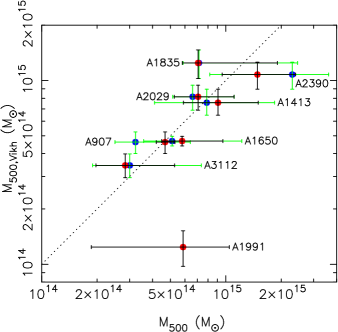
Figure 5.— Cluster masses, $M_{500}$, from Vikhlinin et al. (2005) plotted against those from the clmass model. The unconstrained best fits are shown in blue, with their 90% confidence ranges in green. With the monotonic condition applied, the best fits are shown in red and their 90% confidence ranges in black. 90% confidence ranges are also shown for the masses from Vikhlinin et al. (2005). The dotted line shows equality. No unconstrained result was obtained for Abell 1991.

4.1. Comparison to conventional mass determinations

Fig. 5 compares values of $M_{500}$ determined from the clmass model to those obtained by Vikhlinin et al. (2006) using essentially the same spectra. The figure shows 90% confidence ranges ($\Delta\chi^{2}=2.706$) for both the case where the gravitating matter density is unconstrained (best fit blue, confidence range green) and when it is constrained to be monotonically decreasing (best fit red, confidence range black). Plainly, the clmass model does not place tight limits on values of $M_{500}$ for the sample clusters. For the unconstrained fits, the 90% confidence intervals typically extend over a factor of $\sim 3.5$ in mass.

The situation improves when the monotonic constraint is applied. Apart from Abell 1991, the average length of the 90% confidence ranges is a factor of $\simeq 2.3$ in mass (averaged in log space), compared to $\simeq 1.34$ (i.e., $\delta M/M\simeq 30\%$) for the model-dependent results of Vikhlinin et al. (2005). The formal agreement between the clmass results and Vikhlinin et al. is good, apart from Abell 1991. The clmass value of $M_{500}$ is high for such a cool cluster, stemming from a temperature for the outermost shell inside $r_{500}$ that is high ($kT\simeq 8\pm 4$ keV, $1\sigma$, compared to a projected temperature of $\simeq 2$ keV). With a sample of 8 clusters, it is reasonable to expect disagreement at the 90% level in one case. However, the poor result for Abell 1991 mainly reflects inadequate data at $r_{500}$ and beyond. This result highlights the more general issue for the clmass model, that the total mass is only well-constrained if we have good X-ray data for annuli inside and outside the radius of interest. The lack of better data from beyond $r_{500}$ is the primary cause of the large 90% confidence intervals for $M_{500}$.

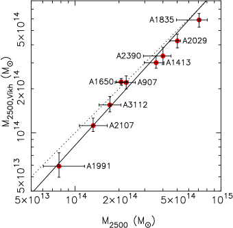
Figure 6.— Cluster masses, $M_{2500}$, from Vikhlinin et al. (2005) versus those from the clmass model. Best fitting results from clmass with the monotonic condition and their 90% confidence ranges are plotted in $x$ and results from Vikhlinin et al. (2005) with their 90% confidence intervals are plotted in $y$. The dotted line shows equality and the full line shows the best fitting straight line.

Masses are better determined at smaller radii, where we have good data from beyond the radius of interest. For the sample clusters, $r_{2500}$ is roughly half of $r_{500}$ (Table 1). Values of $M_{2500}$ from monotonic clmass model fits are compared to the results of Vikhlinin et al. (2005) in Fig. 6. The results for $M_{2500}$ are markedly more accurate than those for $M_{500}$, clearly demonstrating the benefit of having high quality spectra that bracket the radius of interest. Reflecting the greater freedom of the model, 90% confidence ranges from clmass remain larger than those for the model-dependent masses, with a mean spread for the sample of $45\%$, compared to $25\%$ for the model-dependent masses. Individual values of $M_{2500}$ also agree well with the results of Vikhlinin et al. (2005).

There is a modest offset between the clmass results overall and those of Vikhlinin et al. Using the bisector method of Akritas & Bershady (1996) to fit the relationship between the masses

$$\log_{10}{M_{2500,\rm Vikh}\over 10^{14}M_{\odot}}=a+b\log_{10}{M_{2500}\over 10^{14}M_{\odot}}$$ (13)

gives $a=-0.086$ and $b=1.101$, which is plotted in Fig. 6. Monte Carlo simulations using the masses from Vikhlinin et al. (2005) and the fitted errors from both methods show that $b$ is within one standard deviation of unity. However, at the sample mean (in log space), the fitted relationship gives masses that are $12\%$ low (i.e., the clmass results are high), which occurs by chance about 2% of the time. Thus, there is a moderately significant offset between the values of $M_{2500}$ obtained by Vikhlinin et al. and those obtained here.

As noted above, the annuli used here are wider than ideal, so that the mass profile used by the clmass model is coarsely sampled. The gravitational potential, $\Delta\Phi=\int_{a}^{b}GM(r)/r^{2}\,dr$, is more sensitive to mass in the inner part of a shell than the outer part, but, relative to a matter density distribution that decreases with radius, the constant density approximation used by clmass puts more mass in the outer part. Thus, slightly more mass is required in the coarsely sampled clmass model to obtain the same change in gravitational potential. Since the distribution of gas density (i.e., X-ray emission) is determined by the gravitational potential, that is the physical quantity which is fixed by fitting the X-ray data. As a result, the coarsely sampled clmass model finds masses that are biased slightly high. An estimate of this effect is derived in the Appendix and the bias is found to be no more than $\simeq 3\%$. Allowing for the bias expected for $\eta=2$ (see Appendix), the likelihood of the observed 12% bias at the mean mass is increased from about 2% to $\simeq 7\%$. We note that the bias due to coarse sampling is quadratic in $(r_{i+1}/r_{i}-1)$, so that it decreases rapidly with finer sampling. The significance of the remaining $\simeq 9\%$ mass bias is marginal. The issue of possible bias in the clmass model will need to be addressed by other means.

4.2. Strengths and Weaknesses

The clmass model can approximate arbitrary distributions of temperature and gravitating matter, but this freedom means that it fails to constrain cluster masses as tightly as other methods of X-ray mass determination employing more restrictive assumptions. Gravitating mass can also move relatively freely between adjacent shells in the clmass model with little impact on the fit. Its performance in this respect can be improved significantly by requiring the gravitating matter density to be a monotonically decreasing function of the radius. This results in smoother mass profiles and reduces confidence intervals for the mass. The effect of adding a relatively weak assumption to the clmass model illustrates the trade offs between the (apparent) precision of mass determinations and the assumptions they rely on.

Using some of the best X-ray data available and insisting that the mass distribution be monotonic, the clmass model still fails to limit $M_{500}$ to within a factor $\simeq 2$ at the 90% confidence level (Fig. 5). However, it gives well-constrained results for $M_{2500}$. The poor results for $M_{500}$ are a consequence of the generality of the model and the relatively poor quality of the X-ray data near and beyond $r_{500}$. This situation will be slow to improve, because X-ray emission is proportional to the square of the gas density, making it decline rapidly at large radii. It suggests that other X-ray mass determinations rely heavily on their model-dependent assumptions to obtain accurate masses at large radii. While the issue is most acute for X-ray data, model-dependent assumptions have the same effect on all mass determinations. A model-dependent prior, such as the assumption that a cluster potential has the NFW form, reduces confidence intervals for its mass. Unless a prior is accurate, confidence ranges for the mass that rely on it will be too optimistic. Discrepancies between mass determinations may be caused by inappropriate priors as much as by failures of the physical assumptions that underlie mass determinations.

Except for clusters that are obviously dynamically active, X-ray mass determinations generally agree well with dynamical masses (Rines et al., 2003) and with masses determined from weak lensing (Mahdavi et al., 2008; Meneghetti et al., 2009), with a modest bias due to departures from hydrostatic equilibrium. Note that the sample of Mahdavi et al. (2008) includes a number of dynamically active clusters, so that their mean bias of $\sim 20\%$ in $M_{500}$ overestimates the bias for relaxed clusters, such as those used here and by Vikhlinin et al. (2009b). Since model-dependent X-ray masses agree as well as expected with other mass determinations, the confidence ranges for $M_{500}$ obtained with the clmass model appear unnecessarily poor. On the other hand, using the excellent X-ray data bracketing $r_{2500}$, the clmass confidence ranges for $M_{2500}$ are not a lot more conservative than those obtained by careful modeling of the X-ray data (Vikhlinin et al., 2005). Until there are better X-ray telescopes, use of the clmass model is probably better restricted to the brighter regions of clusters. The results here indicate that model-dependent X-ray determinations of $M_{500}$ rely, in effect, on extrapolating to $r_{500}$ models that are largely constrained by data at smaller radii. In view of this, using $M_{2500}$ obtained by fitting the clmass model as a proxy for the total mass, also an extrapolation in effect, may serve as well.

As noted (section 3.1), the annuli used here have $\varpi_{j+1}/\varpi_{j}=1.5$, making the gravitating matter density coarsely sampled for the clmass model. While spectra with many photons are needed to obtain accurate temperatures (more so because clmass effectively deprojects the temperatures), binning the data coarsely discards information about the radial distribution of surface brightness that could help to constrain the distribution of gravitating mass. The performance of the clmass model may well be improved by extracting spectra from narrower annuli. It may even be advantageous to bin the data so finely that individual spectra alone have insufficient counts to constrain the temperatures well. Spectral parameters for groups of adjacent shells could be tied, in effect treating them as a single shell for the spectral fits, while exploiting the information from the individual spectra on the distribution of brightness. This and related issues, such as the best choice of fit statistic, remain to be explored.

There is little constraint on the thermal models that can be used for the spherical shells with clmass. In particular, it would be feasible to use multiphase models (e.g. Russell et al., 2008), provided that an appropriately weighted mean temperature is used for the clmass model temperature for each shell. If the multiphase gas in a shell is well-mixed and in local pressure equilibrium at pressure $p$, the appropriate temperature, $\overline{T}$, can be determined from the mean gas density, $\overline{\rho}_{\rm g}$, by $k\overline{T}=\mu m_{\rm H}p/{\overline{\rho}_{\rm g}}$. In terms of the properties of the separate phases, this yields the weighted temperature $\overline{T}=\left(\sum_{q}K_{q}T_{q}^{2}\right)/\left(\sum_{q}K_{q}T_{q}\right)$, where $K_{q}$ is the xspec norm of the $q^{\rm th}$ phase in the shell, $T_{q}$ is its temperature and the sum runs over all gas phases in the shell.

5. Conclusions

A new approach for making X-ray mass determinations of galaxies, groups and clusters of galaxies was introduced. The new method relies on the usual assumptions of hydrostatic equilibrium and spherical symmetry. Cluster gas is also assumed to be isothermal and the gravitating matter density constant in spherical shells centered on a cluster. With sufficient shells, this distribution provides a good approximation to any spherically symmetric distribution of temperature and gravitating matter, so the approach is largely model-independent. It does not require the additional, model-dependent assumptions that are essential to most conventional X-ray mass determinations.

The method has been implemented as an xspec mixing model called clmass. With no further constraints, the model only determines the gravitating mass in individual shells poorly. This behavior is improved significantly by constraining the gravitating matter density to be a monotonically decreasing function of the radius.

The clmass model was used to determine values for $M_{500}$ and $M_{2500}$ for nine relaxed clusters from the sample of Vikhlinin et al. (2005), as far as possible, using the same spectra. While the results for $M_{500}$ agree with those of Vikhlinin et al., the clmass confidence ranges are much larger than those for the more conventional method. This reflects the lack of assumptions about the form of the gravitating matter distribution in clmass and a lack of good X-ray data from regions beyond $r_{500}$. At smaller radii that are bracketed by good X-ray data, the clmass model performs much better. For $M_{2500}$, clmass gives confidence ranges that are only moderately more relaxed than those of Vikhlinin et al. (2005). Individual masses agree well between the two methods, but there is a small offset in the relationship between the two determinations of $M_{2500}$ at the mean mass. This is partly a consequence of the coarse radial sampling of the spectra used here, but there is a marginally significant offset beyond that.

In regions where we have good X-ray data, the new method can determine masses with comparable accuracy to conventional methods, without relying on model-dependent assumptions. Until we have better X-ray data for the faint outer regions of clusters, it will be less useful for determining total cluster masses, other than by using $M_{2500}$, for example, as a proxy for the virial mass. In contrast to most other approaches, the new method allows confidence ranges for the mass to be determined directly from fits to X-ray spectra. The method can be used with a wide range of thermal models for the X-ray emission from individual shells within a cluster, including multiphase models.

Appendix A Coarse Sampling Mass Bias

For the purpose of estimating the mass bias dues to coarse sampling of the distribution of gravitating matter, we consider a model cluster in which the density distribution is a power law, $\rho_{\rm t}(r)\propto r^{-\eta}$, with $\eta<3$. Locally, this serves as a reasonable approximation for more realistic mass distributions. As argued in section 4.1, the gravitational potential determines the gas distribution, so we assume that the potential is most constrained by the data. Thus we need to compare potentials for the “true” cluster and the clmass approximation to it. Corresponding to the power law density distribution, the mass within radius $r$ is

$$M_{\rm t}(r)=M_{{\rm t},i}(r/r_{i})^{3-\eta},$$ (A1)

where $M_{{\rm t},i}$ is the mass within $r_{i}$. For this mass distribution, the change in gravitational potential from $r_{i}$ to $r_{i+1}$ is

$$\Delta\Phi_{{\rm t},i}=\int_{r_{i}}^{r_{i+1}}{GM_{\rm t}(r)\over r^{2}}\,dr={GM_{{\rm t},i}\over r_{i}}{(1+\Delta)^{2-\eta}-1\over 2-\eta},$$ (A2)

where $1+\Delta=r_{i+1}/r_{i}$. Note that for $\eta\to 2$, the expression $[(1+\Delta)^{2-\eta}-1]/(2-\eta)\to\ln(1+\Delta)$ is well behaved.

Now consider the clmass model approximation for this cluster. As for the sample data, we assume that the shell boundaries follow a geometric progression, $r_{i+1}=(1+\Delta)r_{i}$, for all $i$, but we will ignore the cutoff at $i=1$, assuming that the geometric progression continues to $i=-\infty$ to simplify the sums (an accurate approximation). Matching the power law for the true density distribution, we also assume that the mass densities for the clmass model follow the geometric progression

$$\rho_{i+1}/\rho_{i}=(r_{i+1}/r_{i})^{-\eta}=(1+\Delta)^{-\eta}.$$ (A3)

This condition is not strictly required, but, like the power law for the “true” density, it should be a reasonable local approximation. The form (A3) determines the ratio $\Delta M_{i}/M_{i}$ found below (A5), making it critical to our estimate of the mass bias. For the clmass model, the mass in the $i^{\rm th}$ shell is then

$$\Delta M_{i}={4\pi\over 3}\rho_{i}(r_{i+1}^{3}-r_{i}^{3})={4\pi\over 3}\rho_{i}r_{i}^{3}[(1+\Delta)^{3}-1].$$ (A4)

Under our assumptions, we have $\Delta M_{k}=\Delta M_{i}(1+\Delta)^{(k-i)(3-\eta)}$, so that the shell masses form a geometric progression. Thus, the total mass within $r_{i}$ for the clmass model can be summed to give the total mass within $r_{i}$,

$$M_{i}=\sum_{k=-\infty}^{i-1}\Delta M_{k}={\Delta M_{i}\over(1+\Delta)^{3-\eta}-1}.$$ (A5)

The increase in potential in the $i^{\rm th}$ shell is (equation 3)

$$\Delta\Phi_{i}=\left[{GM_{i}\over r_{i}}+{2\pi\over 3}G\rho_{i}r_{i}^{2}\Delta(3+\Delta)\right]{\Delta\over 1+\Delta}$$ (A6)

and using (A4) and (A5) to express $G\rho_{i}r_{i}^{2}$ in terms of $GM_{i}/r_{i}$, this becomes

$$\Delta\Phi_{i}={GM_{i}\over r_{i}}\left[1+{\Delta(3+\Delta)\over 2}{(1+\Delta)^{3-\eta}-1\over(1+\Delta)^{3}-1}\right]{\Delta\over 1+\Delta}.$$ (A7)

If the potential is determined exactly by the data, as argued above, then fitting the clmass model should make $\Delta\Phi_{i}=\Delta\Phi_{{\rm t},i}$. From equations (A2) and (A7), this determines the ratio of the true mass to the mass obtained from the clmass model as

$${M_{{\rm t},i}\over M_{i}}=1-b={2-\eta\over(1+\Delta)^{2-\eta}-1}\left[1+{\Delta(3+\Delta)\over 2}{(1+\Delta)^{3-\eta}-1\over(1+\Delta)^{3}-1}\right]{\Delta\over 1+\Delta}\simeq 1-{\eta(3-\eta)\over 12}\Delta^{2},$$ (A8)

where $b$ is the mass bias. The last form is an approximation showing the lowest order deviation from unity. The clmass model makes the matter density uniform in shells, so there is no bias for a uniform density distribution, i.e., for $\eta=0$. The bias is also zero for $\eta\to 3$, since then the mass is concentrated at the cluster center and $\Delta\Phi_{i}$ is dominated by the potential due to mass inside $r_{i}$, which is determined correctly in clmass. For the cluster sample used here, $\Delta=r_{i+1}/r_{i}-1=0.5$. The bias for $\Delta=0.5$ is overestimated somewhat ($\simeq 60\%$) by the approximation $b\simeq\eta(3-\eta)\Delta^{2}/12$. Nevertheless, $b(\Delta=0.5)$ is maximized for $\eta=1.5$ at $b\simeq 0.030$. Observed values for $\eta$ at $r_{2500}$ are about 2 or a little greater. For $\eta=2$, the model described here gives $b\simeq 0.026$.

References

- Akritas & Bershady (1996) Akritas, M. G. & Bershady, M. A. 1996, ApJ, 470, 706
- Allen et al. (2008) Allen, S. W., Rapetti, D. A., Schmidt, R. W., Ebeling, H., Morris, R. G., & Fabian, A. C. 2008, MNRAS, 383, 879
- Arabadjis et al. (2004) Arabadjis, J. S., Bautz, M. W., & Arabadjis, G. 2004, ApJ, 617, 303
- Arnaud (1996) Arnaud, K. A. 1996, in Astronomical Society of the Pacific Conference Series, Vol. 101, Astronomical Data Analysis Software and Systems V, ed. G. H. Jacoby & J. Barnes, 17–20
- Bradač et al. (2004) Bradač, M., Lombardi, M., & Schneider, P. 2004, A&A, 424, 13
- Churazov et al. (2008) Churazov, E., Forman, W., Vikhlinin, A., Tremaine, S., Gerhard, O., & Jones, C. 2008, MNRAS, 388, 1062
- Girardi et al. (1998) Girardi, M., Giuricin, G., Mardirossian, F., Mezzetti, M., & Boschin, W. 1998, ApJ, 505, 74
- Hoekstra (2003) Hoekstra, H. 2003, MNRAS, 339, 1155
- Limousin et al. (2007) Limousin, M., Richard, J., Jullo, E., Kneib, J., Fort, B., Soucail, G., Elíasdóttir, Á., Natarajan, P., Ellis, R. S., Smail, I., Czoske, O., Smith, G. P., Hudelot, P., Bardeau, S., Ebeling, H., Egami, E., & Knudsen, K. K. 2007, ApJ, 668, 643
- Mahdavi et al. (2008) Mahdavi, A., Hoekstra, H., Babul, A., & Henry, J. P. 2008, MNRAS, 384, 1567
- Mahdavi et al. (2007) Mahdavi, A., Hoekstra, H., Babul, A., Sievers, J., Myers, S. T., & Henry, J. P. 2007, ApJ, 664, 162
- Mamon & Boué (2009) Mamon, G. A. & Boué, G. 2009, MNRAS, 1693
- Markevitch & Vikhlinin (2007) Markevitch, M. & Vikhlinin, A. 2007, Phys. Rep., 443, 1
- Meneghetti et al. (2009) Meneghetti, M., Rasia, E., Merten, J., Bellagamba, F., Ettori, S., Mazzotta, P., & Dolag, K. 2009, ApJ, in press
- Metzler et al. (2001) Metzler, C. A., White, M., & Loken, C. 2001, ApJ, 547, 560
- Nagai et al. (2007) Nagai, D., Vikhlinin, A., & Kravtsov, A. V. 2007, ApJ, 655, 98
- Newman et al. (2009) Newman, A. B., Treu, T., Ellis, R. S., Sand, D. J., Richard, J., Marshall, P. J., Capak, P., & Miyazaki, S. 2009, ApJ, 706, 1078
- Nulsen & Bohringer (1995) Nulsen, P. E. J. & Bohringer, H. 1995, MNRAS, 274, 1093
- Pointecouteau et al. (2005) Pointecouteau, E., Arnaud, M., & Pratt, G. W. 2005, A&A, 435, 1
- Rines et al. (2003) Rines, K., Geller, M. J., Kurtz, M. J., & Diaferio, A. 2003, AJ, 126, 2152
- Russell et al. (2008) Russell, H. R., Sanders, J. S., & Fabian, A. C. 2008, MNRAS, 390, 1207
- Samushia & Ratra (2009) Samushia, L. & Ratra, B. 2009, ApJ, 703, 1904
- Smith et al. (2005) Smith, G. P., Kneib, J., Smail, I., Mazzotta, P., Ebeling, H., & Czoske, O. 2005, MNRAS, 359, 417
- Vikhlinin et al. (2009a) Vikhlinin, A., Burenin, R. A., Ebeling, H., Forman, W. R., Hornstrup, A., Jones, C., Kravtsov, A. V., Murray, S. S., Nagai, D., Quintana, H., & Voevodkin, A. 2009a, ApJ, 692, 1033
- Vikhlinin et al. (2006) Vikhlinin, A., Kravtsov, A., Forman, W., Jones, C., Markevitch, M., Murray, S. S., & Van Speybroeck, L. 2006, ApJ, 640, 691
- Vikhlinin et al. (2009b) Vikhlinin, A., Kravtsov, A. V., Burenin, R. A., Ebeling, H., Forman, W. R., Hornstrup, A., Jones, C., Murray, S. S., Nagai, D., Quintana, H., & Voevodkin, A. 2009b, ApJ, 692, 1060
- Vikhlinin et al. (2005) Vikhlinin, A., Markevitch, M., Murray, S. S., Jones, C., Forman, W., & Van Speybroeck, L. 2005, ApJ, 628, 655
- Voit (2005) Voit, G. M. 2005, Reviews of Modern Physics, 77, 207
- Zhang et al. (2008) Zhang, Y., Finoguenov, A., Böhringer, H., Kneib, J., Smith, G. P., Kneissl, R., Okabe, N., & Dahle, H. 2008, A&A, 482, 451