ON THE DETERMINATION OF EXACT NUMBER OF LIMIT CYCLES IN LIENARD SYSTEMS

Abstract

We present a simpler proof of the existence of an exact number of one or more limit cycles to the Lienard system $\dot{x}=y-F\left(x\right)$, $\dot{y}=-g\left(x\right)$, under weaker conditions on the odd functions $F\left(x\right)$ and $g\left(x\right)$ as compared to those available in literature. We also give improved estimates of amplitudes of the limit cycle of the Van Der Pol equation for various values of the nonlinearity parameter. Moreover, the amplitude is shown to be independent of the asymptotic nature of $F$ as $\left|x\right|\rightarrow\infty$.

Key words and phrases: Autonomous system, Lienard equation, Limit cycle.

2010 Mathematics Subject Classification: 34C07, 70K05

1 Introduction

There has been a considerable interest in the study of the number and nature of limit cycles in a Lienard equation

$$\ddot{x}+f\left(x\right)\dot{x}+g\left(x\right)=0$$ (1)

recently $\left[\text{\cite[cite]{[\@@bibref{}{Zheng Zuo-Huan}{}{}]}}-\text{\cite[cite]{[\@@bibref{}{Llibre Ponce Torres}{}{}]}}\right]$. Limit cycles are isolated periodic curves in the phase plane and arise in numerous applications as self-sustained oscillations which exist even in the absence of external periodic forcing. The equation $\left(\ref{Lienard Eq}\right)$ is usually studied as an autonomous system, called the Lienard system, given by

$$\dot{x}=y-F\left(x\right),\qquad\dot{y}=-g\left(x\right)$$ (2)

where $F\left(x\right)={\displaystyle\int\limits_{0}^{x}}f\left(u\right)du$. The phase plane defined by $\left(\ref{Lienard System}\right)$ is called the Lienard plane. Lienard gave a criterion for the uniqueness of periodic cycles for a general class of equations when $F\left(x\right)$ is an odd function and satisfies a monotonicity condition as $x\rightarrow\infty$. An interesting problem for the system $\left(\ref{Lienard System}\right)$ is the determination of the number of limit cycles for a given odd degree $\left(m\right)$ polynomial $F\left(x\right)$. Lins, Pugh and de Melo [6] conjectured that the system $\left(\ref{Lienard System}\right)$ has at most $N$ limit cycles if $m=2N+1$ or $m=2N+2$. Currently this problem is being investigated by many authors in connection with the still unsolved Hilbert’s 16th problem.

Giacomini and Neukirch [10] have developed a general procedure for constructing a sequence of polynomials whose roots of odd multiplicity are related to the number and location of the limit cycles of equation $\left(\ref{Lienard Eq}\right)$ when $f\left(x\right)$ is an even degree polynomial. They have also given a sequence of algebraic approximations to the equation of each such cycles, although their method is mainly of experimental (numerical) in nature and a rigorous justification is still lacking. Holst and Sundberg [15] have extended Rychkov’s theorem [5] for a class of $F\left(x\right)$ having $5th$ degree polynomial like behaviour. The proof of Richkov’s theorem however requires bifurcation theory. Odani gave a proof on the existence of exactly $N$ limit cycles of the Lienard equation $\left(\ref{Lienard Eq}\right)$ with $g\left(x\right)=x$. His proof does not make use of the bifurcation theory. His method also gave an improved estimate of the amplitude of a limit cycle. Recently there have been some progress in elucidating sufficient conditions extending the previous results. Chen and Chen [12], for instance, proved the Lins-Pugh-de Melo conjecture for Lienard system with function $F$ odd. On the other hand, it has been shown [16] that for suitable polynomial $F$ of degree $7$, the system $\left(\ref{Lienard System}\right)$ has $4$ limit cycles, contradicting the conjecture in [6]. Chen, Llibre and Zhang [17] proved a sufficient condition for existence of exactly $N$ limit cycles for the system $\left(\ref{Lienard System}\right)$ with a general class of $F\left(x\right)$ functions. We investigate an equivalent problem covering, however, a different class of functions $F$ as compared to [17].

In the study on the number of limit cycles several authors have studied the equation $\left(\ref{Lienard Eq}\right)$ in the usual phase plane $($viz. Theorem $7.10-7.12$, Chapter $4$ in $\cite[cite]{[\@@bibref{}{Zhing Tongren Wenzao}{}{}]})$ whereas some considered the Lienard plane [17]. In Theorem $7.10$, Chapter $4$ [4] the function $f$ is taken as a periodic function. Theorem $7.11$ is a generalization of Theorem $7.10$ in which the function $F^{\prime}\left(x\right)=f\left(x\right)$ is a monotone function in certain regions. However Theorem 3 and Theorem 4 in the present paper do not depend upon the monotonicity of $f$. Rather, we have used the monotonicity of $F$. As a consequence, merely the sign of the function $f$ determines the monotonic nature of $F$, and hence determines the number of limit cycles in Lienard system $\left(\ref{Lienard System}\right)$. Thus our results cover a different class of functions than those covered by Theorems $7.10$ and $7.11$ mentioned above. Theorem $7.12$, Chapter $4$ in [4] and the theorem in [17] have been proved on Lienard plane. Both of these results have assumed the existence of $\beta_{j}\in\left[a_{j},a_{j+1}\right]$, $j=2,3,4,\ldots$ such that $F\left(\beta_{j}\right)=F\left(L_{j-1}\right)$ where, $a_{j}$’s are positive roots of $F$ and $L_{j}$’s are unique extremum of $F$ in $\left[a_{j},a_{j+1}\right]$ for $j=1,2,3,\ldots$. However, if we do not get any such $\beta_{j}$ then these results are not applicable. In such situations Theorem 4 in Section 4 of the present paper is still applicable to determine the exact number of limit cycles. One such example is given in section 5.

In this paper we first give a simple but, nevertheless, an important extension of the Lienard’s theorem for the unique limit cycle by removing the unbounded nature of the function $F$ as $x\rightarrow\infty$. Next, in Theorem 3 we prove that the system $\left(\ref{Lienard System}\right)$ has exactly two limit cycles when the odd function $F\left(x\right)$ undergoes two sign changes in $x>0$ and is monotonic not only as $x\rightarrow\infty$, but also near $($actually at the right of$)$ the first zero. However, $g\left(x\right)$ $(g\left(x\right)>0$ for $x>0)$ can be any odd continuous function. Example 6 in support of Theorem 3 reveals clearly the strength of this theorem over analogous results $($e.g. Theorem $5.1)$ of [4]. The new insights gained from Theorem 3 $($and also from Theorem $\ref{Lienard Theorem Extension})$ then provide a general approach in obtaining an existence theorem for multiple limit cycles in a systematic manner. In Theorem 4, we state a set of such conditions for the existence of exactly $N$ limit cycles. Although we are dealing with odd functions $F$ only, there are certain odd functions as shown in Example 7, which satisfy the conditions of Theorem 4 in the current paper but do not satisfy the theorem of [17]. This establishes our claim that the present theorems cover different classes of functions $F$ than those covered in [4] and [17]. Moreover, as stated above, $g\left(x\right)$ here is an odd function while for the theorem of [17] $g\left(x\right)=x$. The second important result that we find in section 3 is an efficient upper estimate of the amplitude of the limit cycle for the system $\left(\ref{Lienard System}\right)$. The values of the amplitudes for the Van der Pol equation are obtained in Example 1, which are much more accurate compared to those in [11] and [14].

The paper is organized as follows. In section 2, we sketch the main steps of the proof of the classical Lienard theorem thus introducing our notations. In section 3, we discuss some special observations leading to an extension of the classical Lienard theorem. Our main result, Theorem 3, on the existence of two limit cycles is proved in section 4. In Theorem 4 we state the sufficient conditions for existence of exactly $N$ limit cycles. An outline of the proof is given in Appendix $($For a detailed proof, see $\cite[cite]{[\@@bibref{}{Palit Datta 2}{}{}]})$. The proof of this general existence theorem is based on an induction method with non-trivial initial hypotheses for $N=1$ and $N=2$. We present some examples in section 5 highlighting the key features of the above theorems. Section 6 contains some concluding remarks.

2 Lienard’s Theorem

Here we present an outline of the Lienard’s Theorem for the sake of completeness. This helps us introducing necessary notations which will be used subsequently.

Theorem 1

The equation $\left(\ref{Lienard Eq}\right)$ has a unique periodic solution if
$\left(i\right)$ $f$ and $g$ are continuous; $\left(ii\right)$ $F$ and $g\left(x\right)$ are odd functions with $g\left(x\right)>0$ for $x>0$; $\left(iii\right)$ $F$ is zero only at $x=0$, $x=a$, $x=-a$ for some $a>0;$ $\left(iv\right)$ $F\left(x\right)\rightarrow\infty$ as $x\rightarrow\infty$ monotonically for $x>a$.

A Brief Sketch of the Proof. The general shape of the path can be obtained from the following observations.

1. Because of the symmetry of the system$\left(\ref{Lienard Eq}\right)$ under $\left(x,y\right)\rightarrow\left(-x,-y\right)$ any periodic orbit is symmetric about the origin.

2. The slope of a phase path is given by

   $$\frac{dy}{dx}=\frac{-g\left(x\right)}{y-F\left(x\right)}\text{.}$$ (3)

   Thus, a phase path is horizontal if $\dfrac{dy}{dx}=0$, i.e. if $g\left(x\right)=0$, i.e. if $x=0$ $\left(\text{by }\left(ii\right)\text{ above}\right)$. Similarly, a phase path is vertical on the curve $y=F\left(x\right)$. Above the curve $y=F\left(x\right)$ we have $\dot{x}>0$ and below $\dot{x}<0$. Moreover, $\dot{y}<0$ for $x>0$ and $\dot{y}>0$ for $x<0$.

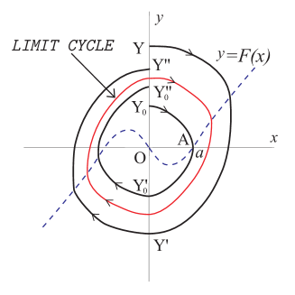
Figure 1: Orbits of the Lienard System $\left(\ref{Lienard System}\right)$.

A path $YY^{\prime}Y^{\prime\prime}$ $($Figure 1$)$ is closed iff $Y$ and $Y^{\prime\prime}$ coincide, which means by symmetry $\left(a\right)$

$$OY=OY^{\prime}\text{.}$$ (4)

This is equivalent to

$$V_{YQY^{\prime}}=0$$ (5)

where for a typical path $YQY^{\prime}$ in Figure 2

$$V_{YQY^{\prime}}=v_{Y^{\prime}}-v_{Y}={\displaystyle\int\limits_{YQY^{\prime}}}dv={\displaystyle\int\limits_{YQY^{\prime}}}Fdy\text{.}$$ (6)

and

$$v\left(x,y\right)={\displaystyle\int\limits_{0}^{x}}g\left(u\right)du+\frac{1}{2}y^{2}\text{.}$$ (7)

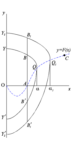
Figure 2: Typical paths for the Lienard Theorem

Writing

$$V_{YQY^{\prime}}=V_{YB}+V_{BQB^{\prime}}+V_{B^{\prime}Y^{\prime}}$$

where $BB^{\prime}$ is a line parallel to the $y-$ axis and passing through the point $\left(0,a\right)$ when the function $F$ changes its sign from negative to positive, one then proves that

1. As $Q$ moves out of the point $A\left(0,a\right)$ along the curve $AC$, the potentials $V_{YB}+V_{B^{\prime}Y^{\prime}}$ is positive and monotone decreasing.

2. As $Q$ moves out of the point $A\left(0,a\right)$ along the curve $AC$, $V_{BQB^{\prime}}$ is monotone decreasing.

3. From $\left(A\right)$ and $\left(B\right)$ it follows that $V_{YQY^{\prime}}$ is monotone decreasing to the right of the point $A$, $($Figure 2$)$.

4. The quantity $V_{BQB^{\prime}}$ tends to $-\infty$ as the paths moves away to infinity.

5. From $\left(C\right)$ and $\left(D\right)$, it follows that the quantity $V_{YQY^{\prime}}$ is monotone decreasing to $-\infty$, at the right of the point $A$ $($Figure 2$)$.

6. $V_{YQY^{\prime}}>0$ when the point $Q$ is at $A$ or to the left of the point $A$.

It thus follows from $\left(E\right)$ and $\left(F\right)$ that $V_{YQY^{\prime}}$ is monotone decreasing continuous function which changes its sign from positive to negative as the point $Q$ moves out of $A\left(a,0\right)$ along the curve. As a result, $V_{YQY^{\prime}}$ will vanish once and only once. Thus, there is one and only one closed path and the proof is complete. $\square$

Remark 1

The unique limit cycle in the above theorem is simple in the sense that no (differentiable) perturbation satisfying the conditions $\left(i\right)$-$\left(iv\right)$ can bifurcate the limit cycle into two or more number of limit cycles.

Remark 2

The condition $\left(E\right)$ enables us to conclude that once $V_{YQY^{\prime}}$ becomes negative, it can never be positive as $Q$ moves to infinity through the curve of $F\left(x\right)$. This observation helps us to deduce the existence of a unique limit cycle. However, we see that the existence of the limit cycle is indeed ensured only if $V_{YQY^{\prime}}$ becomes negative from positive i.e., if there is a change in sign of $V_{YQY^{\prime}}$. Further, the unique value of $x$ for which $V_{YQY^{\prime}}=0$ gives the amplitude of the limit cycle. Accordingly, if $V_{YQY^{\prime}}$ becomes negative as $Q$ moves out from origin through the curve of $F\left(x\right)$ then we get a limit cycle. This observation actually gives one with a possibility of weakening the conditions of the classical theorem, so as to accommodate a larger class of functions $F\left(x\right)$ but still having a unique limit cycle. Theorem 2 is one such realizations of a stronger version of the classical theorem, which shows that the existence of the $($unique$)$ limit cycle actually depends on the local monotonicity of $F\left(x\right)$ on a bounded interval containing the point where $V_{YQY^{\prime}}$ vanishes. A limit cycle can indeed be realized even when $F\left(x\right)$ is bounded as $\left|x\right|\rightarrow\infty$ $($c.f. Example $\ref{Ex Compare Amplitude})$
If it happens further that $V_{YQY^{\prime}}$ becomes positive from negative once more, then also, by an analogous argument as above we can get a point $Q$ on the curve $F\left(x\right)$, through which another limit cycle must pass. To prove this result we consider a function $F\left(x\right)$ $($in section $\ref{New Theorem Section})$ which is monotonically increasing to the right of the point $A$ for a sufficiently large value of $x$ and then it becomes decreasing for some subsequent values of $x$ and ultimately become negative. The proof depends on an efficient estimate of the amplitude of the first limit cycle.

3 Extension of the Classical Theorem and an Estimate of the Amplitude

Let, $\left(\alpha,F\left(\alpha\right)\right)$ be the coordinate of $Q$, as shown in Figure 2 and let $\alpha=\hat{\alpha}$ be the amplitude of the limit cycle of Theorem 1. It is well known that determining the exact value of limit cycle of the Lienard system is a relatively difficult problem $\left[\cite[cite]{[\@@bibref{}{Odani}{}{}]},\cite[cite]{[\@@bibref{}{Lopez}{}{}]}\right]$. We now find an estimate of $\hat{\alpha}$, for which the corresponding $V_{YQY^{\prime}}$ just become negative from positive. Since, $V_{YQY^{\prime}}$ is a monotone decreasing continuous function as the point moves out of the point $A\left(a,0\right)$ along the curve, without any loss of generality we can say $V_{YQY^{\prime}}$ can just become negative from positive if at least one of the following two cases hold, viz.,

$\left(i\right)$ $\ V_{YQ}=0$ but $V_{QY^{\prime}}<0$

$\left(ii\right)$ $V_{QY^{\prime}}=0$ but $V_{YQ}<0$.
The third possibility $V_{YQ}<0$ and $V_{QY^{\prime}}<0$ can be reduced to either of the above two cases by monotonicity and continuity of $V_{YQY^{\prime}}$, i.e. by taking an $\alpha$ closer to $\hat{\alpha}$, $($i.e., $\alpha\rightarrow\hat{\alpha}+0$ $)$ either one of $V_{YQ}$ and $V_{QY^{\prime}}$ can be made to vanish. Similarly, the possibility that either one of $V_{YQ}$ and $V_{QY^{\prime}}$ is positive while their sum is negative, can also be eliminated by choosing $\alpha$ far from $\hat{\alpha}$ $\left(\alpha>\hat{\alpha}\right)$.

Case $\left(i\right)$

Here $V_{YQ}=0$ is possible if

$$V_{YB}+V_{BQ}=0$$ (8)

In step $\left(A\right)$ of the proof of Theorem 1 it has been proved that $V_{YB}>0$.

We are now going to show that $V_{BQ}<0$.

On the path $BQ$, we have $F\left(x\right)\geq 0$ and $\dfrac{dy}{dt}=\dot{y}=-g\left(x\right)<0$.

Therefore,

$$V_{BQ} ={\displaystyle\int\limits_{BQ}}Fdy={\displaystyle\int\limits_{BQ}}F\frac{dy}{dt}dt$$

$$=-{\displaystyle\int\limits_{BQ}}F\left(x\left(t\right)\right)g\left(x\left(t\right)\right)dt\leq 0\text{.}$$ (9)

Thus, we can say that $\left(\text{\ref{Potential Zero Case I}}\right)$ is true if $\left|V_{YB}\right|=\left|V_{BQ}\right|$

$$\text{i.e., if }\left|v\left(a,y_{+}\left(a\right)\right)-v\left(0,y_{+}\left(0\right)\right)\right|=\left|v\left(\alpha,F\left(\alpha\right)\right)-v\left(a,y_{+}\left(a\right)\right)\right|$$

where $y_{+}\left(0\right)=OY$ $($Figure 2$)$. It is possible if

$${\displaystyle\int\limits_{0}^{a}}g\left(u\right)du+\dfrac{1}{2}y_{+}^{2}\left(a\right)-\dfrac{1}{2}y_{+}^{2}\left(0\right)=-{\displaystyle\int\limits_{a}^{\alpha}}g\left(u\right)du-\dfrac{1}{2}F^{2}\left(\alpha\right)+\dfrac{1}{2}y_{+}^{2}\left(a\right)$$

So, we have

$$G\left(\alpha\right)=\dfrac{1}{2}y_{+}^{2}\left(0\right)-\dfrac{1}{2}F^{2}\left(\alpha\right)$$ (10)

where $G\left(x\right)={\displaystyle\int\limits_{0}^{x}}g\left(u\right)du$.

Let $\alpha=\alpha^{\prime}$ be a root of $\left(\text{\ref{Definition of alfa+}}\right)$ $\left(\text{existence of which is assured by construction}\right)$ so that

$$G\left(\alpha^{\prime}\right)=\dfrac{1}{2}y_{+}^{2}\left(0\right)-\dfrac{1}{2}F^{2}\left(\alpha^{\prime}\right)\text{.}$$ (11)

Case $\left(ii\right)$

Here, $V_{QY^{\prime}}=0$ is possible if

$$V_{QB^{\prime}}+V_{B^{\prime}Y^{\prime}}=0$$ (12)

In step $\left(A\right)$ of the proof of the Theorem 1 it is proved that $V_{B^{\prime}Y^{\prime}}>0$.

Proceeding analogous to case $\left(i\right)$ one establishes that $V_{QB^{\prime}}<0$ and consequently $\left(\ref{Potential Zero Case II}\right)$ is true provided

$$G\left(\alpha\right)=\dfrac{1}{2}y_{-}^{2}\left(0\right)-\dfrac{1}{2}F^{2}\left(\alpha\right)$$ (13)

where $OY^{\prime}=-y_{-}\left(0\right),~{}y_{-}\left(0\right)<0$ $($Figure 2$)$. If $\alpha=\alpha^{\prime\prime}$ be a root of $\left(\text{\ref{Definition of alfa-}}\right)$ we have

$$G\left(\alpha^{\prime\prime}\right)=\dfrac{1}{2}y_{-}^{2}\left(0\right)-\dfrac{1}{2}F^{2}\left(\alpha^{\prime\prime}\right)\text{.}$$ (14)

It now follows that if we take

$$\bar{\alpha}=\max\left\{\alpha^{\prime},\alpha^{\prime\prime}\right\}$$ (15)

then for any value of $\alpha>\bar{\alpha},$ $V_{YQY^{\prime}}\leq 0\$since, $V_{YQY^{\prime}}=V_{YQ}+V_{QY^{\prime}}$. Thus the function $F$ should be monotonic increasing in the interval $a<x\leq\bar{\alpha}$. Notice that the classical Lienard theorem already ensures the existence of such an $\bar{\alpha}$. In the light of the above discussion we can now extend the classical Lienard theorem by weakening the unbounded nature of the function $F$ as stated in the following theorem and cover a more large class of functions.

Theorem 2

The equation $\left(\ref{Lienard Eq}\right)$ has a unique limit cycle if
$\left(i\right)$ $f$ and $g$ are continuous in $\left(-d,d\right)$ for sufficiently large $d$; $\left(ii\right)$ $F$ and $g$ are odd functions with $g\left(x\right)>0$ for $x>0$; $\left(iii\right)$ $F$ is zero only at $x=0$, $x=a$, $x=-a$ for some $a$ where $0<a<d;$ $\left(iv\right)$ $\exists$ a number $\bar{\alpha}$ defined by $\left(\ref{Definition of alfaBar}\right)$ such that $F$ is monotonic increasing in $a<x\leq\bar{\alpha}$ and nondecreasing in $\bar{\alpha}<x<d$.

The existence of $\bar{\alpha}$ ensures a sign change in $V_{YQY^{\prime}}$ whereby we get the existence of a unique limit cycle in the finite phase plane. The remaining part of the proof of this theorem remain same as that of classical Lienard theorem. Also, from the above discussion and the proof of classical Lienard theorem it follows that $V_{YQY^{\prime}}$ does not change its sign any more if the function $F$ is simply monotone nondecreasing in $\bar{\alpha}<x<\infty$. In such cases the function $F$ can even be bounded and even attain a constant value as $x\rightarrow\infty$, but still we get a unique limit cycle for such a bounded Lienard system. Thus, we can indeed cover a larger class of functions than those covered by the Lienard theorem $($c.f. 1$)$.

In the beginning of the proof of Theorem 1 we observed that above the curve $y=F\left(x\right)$ we have $\dot{x}>0$ and below $\dot{x}<0$. So, the $x$-coordinate of a point on a limit cycle will achieve its maximum absolute value on the curve $y=F\left(x\right)$. Therefore, the amplitude of a limit cycle for the Lienard system is the abscissa of the point $Q$ lying on the curve $y=F\left(x\right)$. Since, for a limit cycle we have $V_{YQY^{\prime}}=0$, so by the construction of $\bar{\alpha}$ it follows that it is an efficient upper estimate of the amplitude of the limit cycle. In the following example we find the values of $\bar{\alpha}$ for the well known Van der Pol equation against different values of $\mu$ and compare them with the results obtained in [11] and [14]. This also gives an example of a bounded Van der Pol equation having same amplitude as that of the standard Van der Pol equation.

Example 1

Here, in the following table we present estimates of the amplitude of the limit cycle for Van der Pol equation in which $F\left(x\right)=\mu\left(\dfrac{x^{3}}{3}-x\right)$ and $g\left(x\right)=x$ for different values of $\mu.$ It is clear that our estimates are reasonably close to the exact $($numerically computed$)$ values $($as reported in $\cite[cite]{[\@@bibref{}{Odani}{}{}]})$. Our values also appear to be much better than the upper bound $2.3233$ of [11] $($the estimated values of [14] are valid only for small $\mu)$. From our numerical estimates it follows that although the estimated values of the amplitude seem to vary irregularly for the moderately large values of $\mu\in\left[0,10\right]$, these are nevertheless bounded above by $2.05$.

$$\mu$$ and

          

We get the same result if we consider the bounded function

$$F\left(x\right)=\left\{\begin{array}[c]{ll}\mu\left(\dfrac{x^{3}}{3}-x\right)&x\in\left(-2.4,2.4\right)\\ \mu\left(\dfrac{(2.4)^{3}}{3}-2.4\right)-\dfrac{4.76\mu}{\sin\left(0.6\right)}\left(\cos\left(0.6\right)-\cos\left(x-3\right)\right)&x\in\left(-3,-2.4\right]\cup\left[2.4,3\right)\\ \mu\left(\dfrac{(2.4)^{3}}{3}-2.4\right)-\dfrac{4.76\mu}{\sin\left(0.6\right)}\left(\cos\left(0.6\right)-1\right)&x\in\left(-\infty,-3\right]\cup\left[3,\infty\right)\end{array}\right.$$

in the whole phase plane or the following function in finite phase plane.

$$F\left(x\right)=\left\{\begin{array}[c]{ll}\mu\left(\dfrac{x^{3}}{3}-x\right)&x\in\left(-2.4,2.4\right)\\ \mu\left(\dfrac{(2.4)^{3}}{3}-2.4\right)-\dfrac{4.76\mu}{\sin\left(0.6\right)}\left(\cos\left(0.6\right)-\cos\left(x-3\right)\right)&x\in\left(-3,-2.4\right]\cup\left[2.4,3\right)\end{array}\right.$$

This also tells that the value of $d$ need not by too large. A limit cycle is assured even for a moderately large $d$.

It follows from this example that the amplitude of the unique limit cycle is independent of the asymptotic behaviour of $F\left(x\right)$ as $x\rightarrow\infty$. Indeed, the amplitude corresponds to the point $Q\left(\hat{\alpha},F\left(\hat{\alpha}\right)\right)$ on the limit cycle for which the integral $V_{YQY^{\prime}}={\textstyle\int\limits_{YQY^{\prime}}}F~{}dy$ vanishes and clearly depends on the form of $F\left(x\right)$ in the finite interval $\left(0,\hat{\alpha}\right)$. To the best of author’s knowledge, this result apparently is not recorded clearly in the literature. We therefore state this observation as the following corollary.

Corollary 2.1

Amplitude of the unique limit cycle of the Lienard system $\left(\ref{Lienard System}\right)$ is independent of the asymptotic behaviour of $F\left(x\right)$ as $\left|x\right|\rightarrow\infty$.

4 The New Theorem

By the observations discussed in last section it is clear that, in the interval $a<\alpha<\bar{\alpha}$ we obtain the limit cycle of Theorems 1 and 2. Moreover, because of the condition $\left(iv\right)$ we see that the limit cycle remains unique. However, if the function does not satisfy this condition, then the limit cycle may not be unique. We now present our new theorem.

Theorem 3

Let $f$ and $g$ be two functions satisfying the following properties.
$\left(i\right)$ $f$ and $g$ are continuous; $\left(ii\right)$ $F$ and $g$ are odd functions and $g\left(x\right)>0$ for $x>0$.; $\left(iii\right)$ $F$ has positive simple zeros only at $x=a_{1}$, $x=a_{2}$ for some $a_{1}>0$ and some $a_{2}>\bar{\alpha}$, $\bar{\alpha}$ being defined by $\left(\ref{Definition of alfaBar}\right)$ and $\bar{\alpha}<L$, where $L$ is the first local maxima of $F\left(x\right)$ in $\left[a_{1},a_{2}\right];$ $\left(iv\right)$ $F$ is monotonic increasing in $a_{1}<x\leq\bar{\alpha}$ and $F\left(x\right)\rightarrow-\infty$ as $x\rightarrow\infty$ monotonically for $x>a_{2};$
Then the equation $\left(\ref{Lienard Eq}\right)$ has exactly two limit cycles around the origin.

Proof: We can get exactly the same observations as we get in observations $\left(a\right)$ and $\left(b\right)$ in beginning of the proof of Theorem 1.

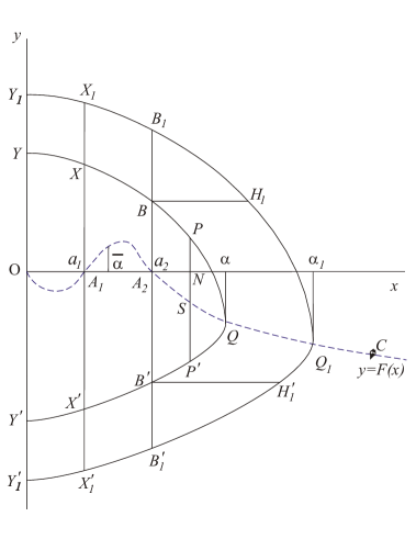
Figure 3:

By the observations in section 3 we can ensure the existence of inner limit cycle. So, we shall now prove the existence of one more limit cycle by showing that

$$OY=OY^{\prime}$$

once more when $x>\bar{\alpha}$. To prove the result we shall consider the function $v\left(x,y\right)$ as in $\left(\ref{Potential Function}\right)$, and write,

$$V_{YQY^{\prime}}=V_{YX}+V_{XB}+V_{BQB^{\prime}}+V_{B^{\prime}X^{\prime}}+V_{X^{\prime}Y^{\prime}}$$ (16)

where, $XX^{\prime}$ is a line parallel to the $y-$ axis passing through the point $\left(0,a_{1}\right)$ where the function $F$ changes its sign from negative to positive and $BB^{\prime}$ is a line parallel to the $y-$ axis passing through the point $\left(0,a_{2}\right)$ where the function $F$ changes its sign from positive to negative. The proof is carried out through the steps $\left(A\right)$ to $\left(F\right)$ below. Here we refer to the Figure 3.

Step $\left(A\right):$ As $Q$ moves out from $A_{2}$ along $A_{2}C$, $V_{YX}+V_{X^{\prime}Y^{\prime}}$ is positive and monotonic decreasing.

We choose two points $Q\left(\alpha,F\left(\alpha\right)\right)$ and $Q_{1}\left(\alpha_{1},F\left(\alpha_{1}\right)\right)$ on the curve of $F\left(x\right)$ where $\alpha_{1}>\alpha$. Let $YQY^{\prime}$ and $Y_{1}Q_{1}Y_{1}^{\prime}$ be two paths through $Q$ and $Q_{1}$ respectively. On the segments $YX$ and $Y_{1}X_{1}$ we have

$$y>0,~{}F\left(x\right)<0\text{ and }y-F\left(x\right)>0\text{.}$$

Now,

$$\left(y-F\left(x\right)\right)_{YX}<\left(y-F\left(x\right)\right)_{Y_{1}X_{1}}$$

Since $g\left(x\right)>0$ for $x>0$, we have

$$\left(\dfrac{-g\left(x\right)}{y-F\left(x\right)}\right)_{YX}<\left(\dfrac{-g\left(x\right)}{y-F\left(x\right)}\right)_{Y_{1}X_{1}}$$

So by $\left(\ref{Gradient of Lienard System}\right)$ we get

$$\left(\dfrac{dy}{dx}\right)_{YX}<\left(\dfrac{dy}{dx}\right)_{Y_{1}X_{1}}<0$$ (17)

Therefore,

$$V_{YX}={\displaystyle\int\limits_{YX}}Fdy={\displaystyle\int\limits_{YX}}\left(-F\right)\left(-\frac{dy}{dx}\right)dx$$

Using $\left(\ref{Gradient Comparison1}\right)$ we get

$$V_{YX}>{\displaystyle\int\limits_{Y_{1}X_{1}}}\left(-F\right)\left(-\frac{dy}{dx}\right)dx$$

Since, $F$ and $dy$ are positive on $Y_{1}X_{1}$ we have

$$V_{YX}>{\displaystyle\int\limits_{Y_{1}X_{1}}}Fdy=V_{Y_{1}X_{1}}>0\text{.}$$ (18)

Next, on the segments $X^{\prime}Y^{\prime}$ and $X_{1}^{\prime}Y_{1}^{\prime}$ we have

$$y<0,~{}F\left(x\right)<0\text{ and }y-F\left(x\right)<0\text{.}$$

Now,

$$\left(y-F\left(x\right)\right)_{X^{\prime}Y^{\prime}}>\left(y-F\left(x\right)\right)_{X_{1}^{\prime}Y_{1}^{\prime}}$$

  

So, by $\left(\ref{Gradient of Lienard System}\right)$

$$\left(\dfrac{dy}{dx}\right)_{X^{\prime}Y^{\prime}}>\left(\dfrac{dy}{dx}\right)_{X_{1}^{\prime}Y_{1}^{\prime}}>0.\ \ \$$ (19)

Therefore,

$$V_{X^{\prime}Y^{\prime}}={\displaystyle\int\limits_{X^{\prime}Y^{\prime}}}Fdy={\displaystyle\int\limits_{Y^{\prime}X^{\prime}}}\left(-F\right)\frac{dy}{dx}dx$$

Using $\left(\ref{Gradient Comparison2}\right)$ we get

$$V_{X^{\prime}Y^{\prime}}>{\displaystyle\int\limits_{Y_{1}^{\prime}X_{1}^{\prime}}}\left(-F\right)\frac{dy}{dx}dx~{}$$

Since, $F$ and $dy$ are negative on $X_{1}^{\prime}Y_{1}^{\prime}$ we have

$$V_{X^{\prime}Y^{\prime}}>{\displaystyle\int\limits_{X_{1}^{\prime}Y_{1}^{\prime}}}Fdy=V_{X_{1}^{\prime}Y_{1}^{\prime}}>0\text{.}$$ (20)

From $\left(\ref{Potential Comparison1}\right)$ and $\left(\ref{Potential Comparison2}\right)$ we have

$$V_{YX}+V_{X^{\prime}Y^{\prime}}>V_{Y_{1}X_{1}}+V_{X_{1}^{\prime}Y_{1}^{\prime}}>0\text{.}$$

Therefore, $V_{YX}+V_{X^{\prime}Y^{\prime}}$ is positive and monotonic decreasing as the point $Q$ moves out from $A_{2}$ along $A_{2}C$.

Step $\left(B\right):$ As $Q$ moves out from $A_{2}$ along $A_{2}C$, $V_{XB}+V_{B^{\prime}X^{\prime}}$ is negative and monotonic increasing.

On the segments $XB$ and $X_{1}B_{1}$ we have

$$y>0,~{}F\left(x\right)<0\text{ and }y-F\left(x\right)>0\text{.}$$

Now,

$$\left(y-F\left(x\right)\right)_{XB}<\left(y-F\left(x\right)\right)_{X_{1}B_{1}}$$

So, by $\left(\ref{Gradient of Lienard System}\right)$ we get

$$\left(\dfrac{dy}{dx}\right)_{XB}<\left(\dfrac{dy}{dx}\right)_{X_{1}B_{1}}<0\ \ \$$ (21)

Therefore,

$$V_{XB}={\displaystyle\int\limits_{XB}}Fdy={\displaystyle\int\limits_{XB}}F\frac{dy}{dx}dx$$

Using $\left(\ref{Gradient Comparison3}\right)$ we get

$$V_{XB}<{\displaystyle\int\limits_{X_{1}B_{1}}}F\frac{dy}{dx}dx={\displaystyle\int\limits_{X_{1}B_{1}}}Fdy=V_{X_{1}B_{1}}<0$$ (22)

since, $F>0$ and $dy<0$ on $XB$ and $X_{1}B_{1}$.

Next, on the segments $B^{\prime}X^{\prime}$ and $B_{1}^{\prime}X_{1}^{\prime}$ we have

$$y<0,~{}F\left(x\right)>0\text{ and }y-F\left(x\right)<0\text{.}$$

Now,

$$\left(y-F\left(x\right)\right)_{B^{\prime}X^{\prime}}>\left(y-F\left(x\right)\right)_{B_{1}^{\prime}X_{1}^{\prime}}$$

Using $\left(\ref{Gradient of Lienard System}\right)$ we get

$$\left(\dfrac{dy}{dx}\right)_{B^{\prime}X^{\prime}}>\left(\dfrac{dy}{dx}\right)_{B_{1}^{\prime}X_{1}^{\prime}}>0.\ \$$ (23)

Therefore,

$$V_{B^{\prime}X^{\prime}}={\displaystyle\int\limits_{B^{\prime}X^{\prime}}}Fdy=-{\displaystyle\int\limits_{X^{\prime}B^{\prime}}}F\frac{dy}{dx}dx={\displaystyle\int\limits_{X^{\prime}B^{\prime}}}F\left(-\frac{dy}{dx}\right)dx$$

So, by $\left(\ref{Gradient Comparison4}\right)$ we have

$$V_{B^{\prime}X^{\prime}}<{\displaystyle\int\limits_{X_{1}^{\prime}B_{1}^{\prime}}}F\left(-\frac{dy}{dx}\right)dx~{}={\displaystyle\int\limits_{B_{1}^{\prime}X_{1}^{\prime}}}Fdy=V_{B_{1}^{\prime}X_{1}^{\prime}}<0\text{.}$$ (24)

since, $F>0$ and $dy<0$ on $B^{\prime}X^{\prime}$ and $B_{1}^{\prime}X_{1}^{\prime}$.

From $\left(\ref{Potential Comparison3}\right)$ and $\left(\ref{Potential Comparison4}\right)$ we have

$$V_{XB}+V_{B^{\prime}X^{\prime}}<V_{X_{1}B_{1}}+V_{B_{1}^{\prime}X_{1}^{\prime}}<0\text{.}$$

Therefore, $V_{XB}+V_{B^{\prime}X^{\prime}}$ is negative and monotonic increasing as the point $Q$ moves out from $A_{2}$ along $A_{2}C$.

Step $\left(C\right):$ As $Q$ moves out from $A_{2}$ along $A_{2}C$, $V_{BQB^{\prime}}$ is positive and monotonic increasing and tends to $+\infty$ as the path recedes to infinity.

On $BQB^{\prime}$ and $B_{1}Q_{1}B_{1}^{\prime}$, we have $F\left(x\right)<0$. We draw $BH_{1}$ and $B^{\prime}H_{1}^{\prime}$ parallel to $x-$ axis.

Therefore,

$$V_{B_{1}Q_{1}B_{1}^{\prime}} ={\displaystyle\int\limits_{B_{1}Q_{1}B_{1}^{\prime}}}Fdy$$

$$={\displaystyle\int\limits_{B_{1}^{\prime}Q_{1}B_{1}}}\left(-F\right)dy$$

$$\geq{\displaystyle\int\limits_{H_{1}^{\prime}Q_{1}H_{1}}}\left(-F\right)dy$$

since, $F\left(x\right)<0$ and $dy>0$ for points on $H_{1}^{\prime}Q_{1}H_{1}$. Again since,

$$\left.F\left(x\right)\right]_{B^{\prime}QB}\geq\left.F\left(x\right)\right]_{H_{1}^{\prime}Q_{1}H_{1}}$$

for same value of $y$ we get

$$V_{B_{1}Q_{1}B_{1}^{\prime}} \geq{\displaystyle\int\limits_{H_{1}^{\prime}Q_{1}H_{1}}}\left(-F\right)dy\geq{\displaystyle\int\limits_{B^{\prime}QB}}\left(-F\right)dy$$

$$={\displaystyle\int\limits_{BQB^{\prime}}}Fdy$$

$$=V_{BQB^{\prime}}$$

$$\implies V_{B_{1}Q_{1}B_{1}^{\prime}}$$

(26)

Next, let $S$ be a point on the curve of $F\left(x\right)$, to the right of $A_{2}$, and let $BQB^{\prime}$ be an arbitrary path, with $Q$ to the right of $S$. The straight line $PNSP^{\prime}$ is parallel to the $y-$ axis. Then,

$$V_{BQB^{\prime}} ={\displaystyle\int\limits_{BQB^{\prime}}}F\left(x\right)dy$$

$$={\displaystyle\int\limits_{B^{\prime}QB}}\left(-F\left(x\right)\right)dy$$

$$\geq{\displaystyle\int\limits_{P^{\prime}QP}}\left(-F\left(x\right)\right)dy$$ (27)

since, $\left(-F\left(x\right)\right)\geq 0$ and $dy\geq 0$ along $B^{\prime}QB$. Now by condition $\left(iv\right)$ of this theorem it follows that $F$ is monotonic decreasing for $x>a_{2}$ and so we have $\left|F\left(x\right)\right|\geq NS$ on $P^{\prime}QP$ and since further $F\left(x\right)\leq 0$ on $P^{\prime}QP$ so this implies $-F\left(x\right)\geq NS$ on $P^{\prime}QP$. Again, $PP^{\prime}\geq NP^{\prime}$. Thus we get

$$V_{BQB^{\prime}}\geq{\displaystyle\int\limits_{P^{\prime}QP}}NS~{}dy=NS{\displaystyle\int\limits_{P^{\prime}QP}}dy=NS\cdot PP^{\prime}\geq NS\cdot NP^{\prime}~{}\text{.}$$

But as $Q$ goes to infinity towards the right , $NP^{\prime}\rightarrow\infty$. Hence, we can conclude that $V_{BQB^{\prime}}$ is positive and monotonic increasing and tends to $+\infty$ as the paths recede to infinity.

Step $\left(D\right):$

From steps $\left(A\right)$ and $\left(B\right)$ it follows that the quantities $V_{YX}+V_{X^{\prime}Y^{\prime}}$ and $V_{XB}+V_{B^{\prime}X^{\prime}}$ are bounded quantities. Thus by $\left(\ref{Potential Decomposition}\right)$ and by step $\left(C\right)$ it follows that $V_{YQY^{\prime}}$ is monotonic increasing to $+\infty$ to the right of $A_{2}$.

Step $\left(E\right):$

By the construction of $\bar{\alpha}$ it is clear that $V_{YQY^{\prime}}<0$ in $\bar{\alpha}\leq x<a_{2}$ i.e., to the left of $A_{2}$. Again from step $\left(D\right)$ we conclude that $V_{YQY^{\prime}}$ ultimately becomes positive as $Q$ moves out of $A_{2}$ along the curve of $F\left(x\right)$. Therefore, by the same reason given in conclusion of the Theorem 1, it follows that there is one and only one path in the region $x>\bar{\alpha}$ such that

$$V_{YQY^{\prime}}=0\text{.}$$

Also, by $\left(\ref{Potential Zero}\right)$ and the symmetry of the path it is clear that the path is closed.

Step $\left(F\right):$

By the construction of $\bar{\alpha}$ and by step $\left(E\right)$ it is clear that equation $\left(\ref{Lienard Eq}\right)$ has exactly two limit cycles around the origin, the second limit cycle surrounds the first one. This completes the proof of the Theorem 3.

Remark 3

It also follows from the proof that both the limit cycles are simple $($c.f., Remark $\ref{Simple Limit Cycle})$ that neither can bifurcate under any small $C^{1}$ perturbation satisfying the conditions of the theorem

Remark 4

One cannot assume that $V_{YQY^{\prime}}<0$ if $\bar{\alpha}\geq L$. We give a counter example below.

Remark 5

It is well known that two consecutive limit cycle cannot both be stable $\left(\text{unstable}\right)$. Because of our choice of the function $F\left(x\right)$ $($negative and monotone decreasing at the right of and near the origin and infinity$)$, the inner limit cycle is stable and outer limit cycle is unstable $($in reverse to those of reference $\left[\cite[cite]{[\@@bibref{}{Odani N}{}{}]}\text{, }\cite[cite]{[\@@bibref{}{Holst Sunburg}{}{}]}\right])$.

The existence of exactly $N$ limit cycles is established by an easy extension of the above proof [19]. We state the theorem as follows. A brief outline of its proof is given in the Appendix.

Theorem 4

Let $f$ and $g$ be two functions satisfying the following properties.
$\left(i\right)$ $f$ and $g$ are continuous; $\left(ii\right)$ $F$ and $g$ are odd functions and $g\left(x\right)>0$ for $x>0$.; $\left(iii\right)$ $F$ has $N$ number of positive simple zeros only at $x=a_{i}$, $i=1,2,\ldots,N$ where $0<a_{1}<a_{2}<\ldots<a_{N}$ such that in each interval $I_{i}=\left[a_{i},a_{i+1}\right]$, $i=1,2,\ldots,N-1$, there exists $\bar{\alpha}_{i}$, satisfying properties given by $\left(\text{\ref{Definition of alfaBar}}\right)$, such that $\bar{\alpha}_{i}<L_{i}$ where $L_{i}$ is the unique extremum in $I_{i}$, $i=1,\ldots,N-2$ and $L_{N-1}$, the first local extremum in $\left[a_{N-1},a_{N}\right]$. $\left(iv\right)$ $F$ is monotonic in $a_{i}<x\leq\bar{\alpha}_{i}$ $\forall$ $i$ and $\left|F\left(x\right)\right|\rightarrow\infty$ as $x\rightarrow\infty$ monotonically for $x>a_{N}$.
Then the equation $\left(\text{\ref{Lienard Eq}}\right)$ has exactly $N$ limit cycles around the origin, all are simple.

Remark 6

The conditions $\left(i\right)$ and $\left(iv\right)$ of Theorem 3 and Theorem 4 may be weakened following Theorem 2. For instance, the condition $\left(iv\right)$ of Theorem 3 may be restated as
$\left(iv\right)$ $F$ is monotonic increasing in $a_{1}<x\leq\bar{\alpha}=\bar{\alpha}_{1}$ $\left(\text{say}\right)$ and $\exists$ a number $\bar{\alpha}_{2}$ given by $\left(\ref{Definition of alfaBar}\right)$ such that $F$ is monotonic decreasing in $a_{2}<x\leq\bar{\alpha}_{2}$ and nonincreasing in $\bar{\alpha}_{2}<x<d$.

5 Examples

It is shown in section 3.3 of [15] that the limit cycles of the autonomous system

$$\left.\begin{array}[c]{c}\dot{x}=y\\ \dot{y}=-x-\mu h\left(x,\dot{x}\right)\end{array}\right\}$$ (28)

are asymptotic to the circle $x^{2}+y^{2}=r^{2}$ as $\mu\rightarrow 0$ where the values of $r$ are the roots of the equation

$$\Phi\left(r\right):=\int_{0}^{2\pi}h\left(r\sin u,r\cos u\right)\cos u~{}du=0\text{.}$$ (29)

We note that this is not the Lienard system. It is the canonical phase plane for Lienard equation. The phase diagram of above system and the Lienard system, however, should be similar. Here we take $\mu=0.1,$ $h\left(x,\dot{x}\right)=\left(-4+75x^{2}-50kx^{4}\right)\dot{x},$ $k\neq 0$ so that

$$f\left(x\right)=\mu\left(-4+75x^{2}-50kx^{4}\right)=-0.4+7.5x^{2}-5kx^{4}$$

$$F\left(x\right)=-0.4x+2.5x^{3}-kx^{5}$$

and

$$\Phi\left(r\right) =\int_{0}^{2\pi}\left(-4+75r^{2}\sin^{2}u-50kr^{4}\sin^{4}u\right)r\cos u\cdot\cos u~{}du$$

$$=-\frac{1}{4}\pi r\left(25kr^{4}-75r^{2}+16\right)\text{.}$$

Therefore, $\left(\ref{Definition of phi}\right)$ reduces to

$$-\frac{1}{4}\pi r\left(25kr^{4}-75r^{2}+16\right)=0$$

giving

$$r^{2}=\frac{1}{10k}\left(15\pm\sqrt{225-64k}\right)\text{.}$$

So, $\left(\ref{Definition of phi}\right)$ has real and distinct roots if $225>64k$ i.e., if $k<3.515625$, real and repeated if $k=3.515625$ and imaginary if $k>3.515625$. Therefore it follows that we will get two distinct limit cycles, which are asymptotic to the circles corresponding to the above two distinct values of $r$ if $k<3.515625$. Similarly, we will get only one limit cycle when $k=3.515625$ and no limit cycle when $k>3.515625$. It can be verified that the system undergoes a saddle node bifurcation at $k=3.515625$.

We note that the point $\left(\bar{\alpha},F\left(\bar{\alpha}\right)\right)$ on the limit cycle in the Lienard plane gets transformed to the point $\left(-\bar{\alpha},0\right)$ lying on the almost circular limit cycle of radius $r\gtrsim r_{1}$ $($in the canonical phase plane$)$ where $r_{1}^{2}=\frac{1}{10k}\left(15-\sqrt{225-64k}\right)$ $(r_{1}$ corresponds to the first limit cycle$)$ under the transformation

$$x=-u,~{}y=-v+F\left(u\right)$$

$\left(u,v\right)$ and $\left(x,y\right)$ being the corresponding points in Lienard plane and canonical phase plane with $f$ an even function. We thus have

$$\bar{\alpha}\gtrsim\sqrt{\frac{1}{10k}\left(15-\sqrt{225-64k}\right)\text{.}}$$

We now present the phase diagrams of the above systems in Lienard plane in the following examples for different values of $k$. These examples justify our new theorem. We use Mathematica 5.1 in constructing the examples.

Example 2

Here we consider the autonomous system $\left(\ref{Lienard System}\right)$ with $k=3.65$, $f\left(x\right)=-0.4+7.5x^{2}-5kx^{4}$ $g\left(x\right)=x$ and $F\left(x\right)=-0.4x+2.5x^{3}-kx^{5}$. The phase diagram in Lienard plane is shown in Figure 4

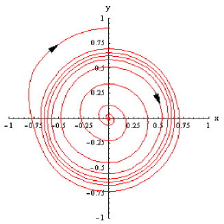
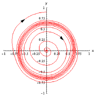
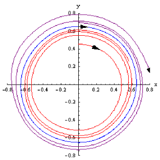
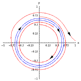
Figure 4: The phase diagram of the system $\left(\ref{Lienard System}\right)$ in Lienard plane
$\left(a\right)$ with $k=3.65$, and center as a repelling node in Example 2,
$\left(b\right)$ with $k=3.57$ in Example 2,
$\left(c\right)$ with $k=3.515625$, and one limit cycle in Example 3,
$\left(d\right)$ with $k=3.5$, and two limit cycles in Example 4.

which does not have any limit cycle. Again we take $k=3.57$ in the above system. The corresponding phase diagram is shown in Figure 4. This phase diagram also does not contain any limit cycle, but we see that the path is concentrating in a certain circular region.

Example 3

Here we consider the autonomous system $\left(\ref{Lienard System}\right)$ discussed above with $k=3.515625$ so that $a_{1}\simeq 0.49307$, $a_{2}\simeq 0.68410$, $y_{+}\left(0\right)$ and $y_{-}\left(0\right)$ both are approximately equal to $0.652287$ and $\bar{\alpha}\simeq 0.65204$. Let $L_{1}$ be the point of minima of $F$ in $\left(0,a_{1}\right)$ and $L_{2}$ be the point of maxima of $F$ in $\left(a_{1},a_{2}\right)$. Here $F\left(x\right)$ is increasing in

$$\left(-L_{2},L_{1}\right)\cup\left(L_{1},L_{2}\right)$$

and decreasing in

$$\left(-\infty,-L_{2}\right)\cup\left(-L_{1},L_{1}\right)\cup\left(L_{2},\infty\right)$$

where, $L_{1}\simeq 0.24997$ and $L_{2}\simeq 0.60348$. In this case we obtain only one limit cycle as shown in Figure 4. Here, $F$ is not monotone increasing throughout the interval $a_{1}<x\leq\bar{\alpha}$, violating the condition $\left(iv\right)$ of Theorem 3 $($since $\bar{\alpha}>L_{2})$.

Example 4

We now take $k=3.5$. Here, $y_{+}\left(0\right)$ and $y_{-}\left(0\right)$ are approximately equal to $0.624499$. The equations $\left(\ref{Definition of alfa+}\right)$ and $\left(\ref{Definition of alfa-}\right)$ both reduce to

$$\frac{x^{2}}{2}=\frac{1}{2}\left(0.624499\right)^{2}-\frac{1}{2}\left(-0.4x+2.5x^{3}-3.5x^{5}\right)^{2}$$

having real roots $x=\pm 0.62393$ so that $\bar{\alpha}\simeq 0.62393$. Here, $a_{1}=0.4919$ and $a_{2}=0.68725$ showing that $a_{1}<\bar{\alpha}<a_{2}$. Next, $L_{1}\simeq 0.24985$, $L_{2}\simeq 0.60510$. Here all the conditions of Theorem 3 are satisfied except condition $\left(iv\right)$. However we still get two limit cycles as shown in Figure 4 drawn in Lienard plane. This example and the above example show that the conditions of Theorem 3 are sufficient but not necessary.

Example 5

Finally we take $k=3$. Here, $y_{+}\left(0\right)$ and $y_{-}\left(0\right)$ are approximately equal to $0.5552$ and $\bar{\alpha}\simeq 0.55324$. Here, $a_{1}=0.46473$ and $a_{2}=0.78572$ showing that $a_{1}<\bar{\alpha}<a_{2}$. Next, $L_{1}\simeq 0.24638$, $L_{2}\simeq 0.66279$. Here, all the conditions of Theorem 3 are satisfied and so we get exactly two limit cycles. The phase diagram in Lienard plane is shown in Figure 5.

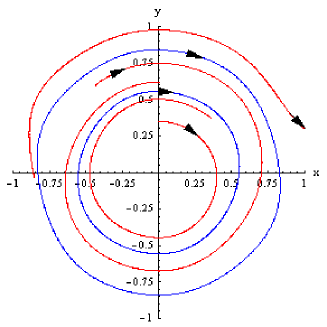
Figure 5: The phase diagram of the system $\left(\text{\ref{Lienard System}}\right)$ in Lienard plane with $k=3$, and two limit cycles in Example 5.

Remark 7

Although in the above examples the value of $\mu$ is sufficiently small $($so as to satisfy the amplitude analysis of $\cite[cite]{[\@@bibref{}{Holst Sunburg}{}{}]})$ our theorem should be applicable for large values of $\left|\mu\right|$. More detailed bifurcation analysis in the $\left(\mu,k\right)$ parametric plane will be considered separately.

Example 6

We now consider the function

$$F_{+}\left(x\right)=\left\{\begin{array}[c]{ll}-0.1\sin\left(10\pi x\right)&0\leq x<0.15\\ 0.01\sqrt{1-\left(\dfrac{x-0.15}{0.01}\right)^{2}}&0.15\leq x<0.15+\dfrac{1}{\sqrt{101}}\\ \begin{array}[c]{l}0.02099503719021-\\ \hskip 36.135pt2\sqrt{0.1\left(x-0.2395037190209989\right)}\end{array}&x\geq 0.15+\dfrac{1}{\sqrt{101}}\end{array}\right.$$

Then we have $a_{1}=0.1$, $a_{2}=0.25052350868645645$, $L=0.15$. Here,

$$f\left(L\right)=0<f\left(0.2395037190209989\right)=0.2006848039831627>f\left(a_{2}\right)=0.9526060763219791,$$

though

$$L<0.2395037190209989<a_{2}$$

showing that the function is not monotone nonincreasing in $\left[L,a_{2}\right]$ and so it does not satisfy the condition $\left(3\right)$ of Theorem $5.1$ in chapter $4$ in the book [4]. However for the inner limit cycle we have $y_{+}\left(0\right)=y_{-}\left(0\right)=0.12238318$. So, $\bar{\alpha}=0.12221435874426823<L$ satisfying the conditions of Theorem 3. This example clearly shows that the Theorem 3 covers a larger class of functions than those covered by Theorem $5.1$ in chapter $4$ in [4]. The function $F$ alongwith two limit cycles are shown in Figure 6.

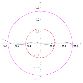
Figure 6: The phase diagram of $\left(\text{\ref{Lienard System}}\right)$ in Lienard plane for Example 6.

Example 7

We now consider a different problem. Here we define

$$F_{+}\left(x\right)=\left\{\begin{array}[c]{ll}0.005-0.025\sqrt{1-\left(\dfrac{x-0.048989794}{0.05}\right)^{2}}&0\leq x<a_{1}\\ -0.0008137888130718+0.01\sqrt{1-\left(\dfrac{x-0.14781375}{0.05}\right)^{2}}&a_{1}\leq x<a_{2}\\ 0.0009168416064002765-0.015\sqrt{1-\left(\dfrac{x-0.29746094}{0.1}\right)^{2}}&a_{2}\leq x<a_{3}\\ -0.0003265987749816556+0.04\sqrt{x-0.3972073012751128}&x\geq a_{3}\end{array}\right.$$

where

$$a_{1} =0.097979588$$

$$a_{2} =0.197647912$$

$$\text{and }a_{3} =0.397273968.$$

and

$$F\left(x\right)=\left\{\begin{array}[c]{lc}F_{+}\left(x\right)&x\geq 0\\ -F_{+}\left(-x\right)&x<0\end{array}\right.$$

The function $F_{+}\left(x\right)$ is obtained by matching three ellipses and a parabola successively in the intervals $\left(0,a_{1}\right),$ $\left(a_{1},a_{2}\right),$ $\left(a_{2},a_{3}\right),$ and $\left(a_{3},\infty\right)$ such that

$$F_{+}\left(a_{i}+0\right)=F_{+}\left(a_{i}-0\right)\text{ and }F_{+}^{\prime}\left(a_{i}+0\right)=F_{+}^{\prime}\left(a_{i}-0\right),$$ (30)

where $a_{i}$’s are zeros of $F_{+}$. The unique extremum of $F$ in $\left(0,a_{1}\right)$, $\left(a_{1},a_{2}\right)$, $\left(a_{2},a_{3}\right)$ are respectively

$$L_{0} =0.048989794$$

$$L_{1} =0.14781375$$

$$\text{and }L_{2} =0.29746094.$$

We obtain three limit cycles which meet the positive $y$-axis at the points $\left(0,y_{1}\left(0\right)\right)$, $\left(0,y_{2}\left(0\right)\right)$, $\left(0,y_{3}\left(0\right)\right)$ where

$$y_{1}\left(0\right) =0.1332869$$

$$y_{2}\left(0\right) =0.212146685$$

$$\text{and }y_{3}\left(0\right) =0.4630114\text{.}$$

The matching conditions $\left(\ref{Matching Cond}\right)$ are used to make $F\in C^{1}\left(R\right)$ with accuracy level $O\left(10^{-7}\right)$. This function is constructed in a trial and error method and numerical data with large significant digits arise in this fashion. Examples with lower significant digits and lower and higher accuracy are possible in principle. Here we get $\bar{\alpha}_{1}=0.133002186$ and $\bar{\alpha}_{2}=0.21203506657$. The function $F$ satisfies all the conditions of Theorem 4 $($for example $\bar{\alpha}_{i}<L_{i}$ etc.$)$ and so the existence of the above three limit cycles are ensured by this theorem, the proof of which is presented separately [19]. However, the function $F$ is defined in such a manner that $\left|F\left(L_{0}\right)\right|>\left|F\left(L_{2}\right)\right|$ implying that $\beta_{2}$ mentioned in Theorem $1$ of [17] or in Theorem $7.12$, chapter $4$ of the book [4] does not exist and hence these theorems are not applicable for the corresponding Lienard system. The limit cycles of the Lienard system in Lienard plane and the graph of the function $F$ have been shown separately in the Figure 7. To conclude, Theorem $1$ of [17] or Theorem $7.12$, Chapter $4$ in the book [4] fail to predict the existence of the exact number of limit cycles for the above function $F\left(x\right)$.

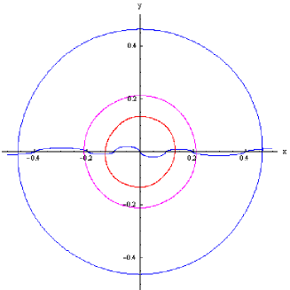
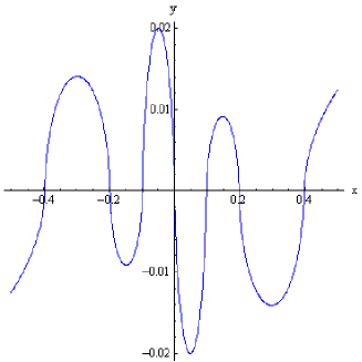
Figure 7: $\left.{}\right.\newline \left(a\right)$ The phase diagram of the system $\left(\ref{Lienard System}\right)$ in Lienard plane with three limit cycles.
$\left(b\right)$ Graph of the function $F$ in Example 7.

6 Concluding Remarks

Many interesting new results have been proved on the existence of an exact number of multiple limit cycles $\left[\cite[cite]{[\@@bibref{}{Odani N}{}{}]},\cite[cite]{[\@@bibref{}{Holst Sunburg}{}{}]},\cite[cite]{[\@@bibref{}{Chen Llibre Zhang}{}{}]}\right]$ in the recent past. Odani has proved a sufficient condition in [8] using a choice function $\phi_{k}$ which can be exploited to obtain better estimates of amplitudes of the limit cycles. We used a straight forward method depending on the geometry of phase diagram. We have proved a similar result with more general class of functions $F\left(x\right)$ by a simpler method. In the present approach a strict monotonicity of $F\left(x\right)$ is required only in the intervals $a_{1}<x<\bar{\alpha}$ and $x>a_{2}$. Consequently, $F\left(x\right)$ can accommodate “small scale” oscillations in the interval $\bar{\alpha}<x<a_{2}$. Odani, for instance, considered an $F\left(x\right)$ which is not only $C^{1}$ but also has a unique extremum in the interval $a_{1}<x<a_{2}$. Further, the theorem is valid for a more general class of the function $g\left(x\right)$. Odani’s theorem however is valid only for $g\left(x\right)=x$. An interesting problem will be to establish the relation between $\bar{\alpha}$ of our approach and the function $\phi_{k}$. We note that $\hat{\alpha}_{i}$ corresponds to the amplitude of the limit cycles. Our estimates of amplitude of the limit cycle of the Van der pol equation constitute an improvement over those available in the literature $\left[\cite[cite]{[\@@bibref{}{Odani}{}{}]},\text{ }\cite[cite]{[\@@bibref{}{Lopez}{}{}]}\right]$. Examples 6 & 7, on the other hand, show the difference between the present theorem and those of [4] and [17]. The calculations are accurate upto the accuracy level $O\left(10^{-7}\right)$. The existence of limit cycles in a Lienard system allowing discontinuity $($see, for instance, $\cite[cite]{[\@@bibref{}{Llibre Ponce Torres}{}{}]})$ is an interesting problem for further study. Determining the shape of the limit cycles is also left for future investigations.

Before closing we note that the value $\bar{\alpha}$, in general, is a function of the parameters of $F\left(x\right)$ in the parametric space. For instance, in Examples $\ref{Ex1}-\ref{Ex4}$, $\bar{\alpha}$ is a function of the parameters $\mu$ and $k$. The study of the variation of $\bar{\alpha}$ in the parametric space seems to offer interesting insights into the bifurcation and related issues of the multiple limit cycles in a Lienard system. The relationship with Poincare’s return map also needs to be studied. We wish to investigate these problems in future.

7 Appendix

Here we present a brief outline of the proof of Theorem 4 which is given in detail in [19]. The theorem is proved by an induction method which is dependent on the non-trivial initial hypotheses that the the result holds for $N=1$ and $N=2$.

Figure 8:

We shall prove the theorem by showing the result that each limit cycle intersects the $x-$axis at a point lying in the open interval $\left(\bar{\alpha}_{i},\bar{\alpha}_{i+1}\right]$, $i=0,1,2,\ldots,N-1$, where $\bar{\alpha}_{0}=L_{0}$ is the local minima of $F\left(x\right)$ in $\left[0,a_{1}\right]$. By Lienard theorem and Theorem 3 it follows that the result is true for $N=1$ and $N=2$. We shall now prove the theorem by induction. We assume that the theorem is true for $N=n-1$ and we shall prove that it is true for $N=n$. We prove the theorem by taking $n$ as an odd $+ve$ integer so that $\left(n-1\right)$ is even. The case for which $n$ is even can similarly be proved and so is omitted. It can be shown that [1], $V_{YQY^{\prime}}$ changes its sign from $+ve$ to $-ve$ as $Q$ moves out of $A_{1}\left(a_{1},0\right)$ along the curve $y=F\left(x\right)$ and hence vanishes there due to its continuity and generates the first limit cycle around the origin. Next, in Theorem 3 we see $V_{YQY^{\prime}}$ again changes its sign from $-ve$ to $+ve$ and generates the second limit cycle around the first. Also, we see that for existence of second limit cycle we need the existence of the point $\bar{\alpha}$, which we denote here as $\bar{\alpha}_{1}$.

Since by induction hypothesis the theorem is true for $N=n-1$, so it follows that in each and every interval $\left(\bar{\alpha}_{k},\bar{\alpha}_{k+1}\right]$, $k=0,1,2,\ldots,n-2$ the system $\left(\ref{Lienard System}\right)$ has a limit cycle and the outermost limit cycle cuts the $x-$ axis somewhere in $\left(\bar{\alpha}_{n-1},\infty\right)$. Also $V_{YQY^{\prime}}$ changes its sign alternately as the point $Q$ moves out of $a_{i}$’s, $i=1,2,\ldots,n-1$. Since $\left(n-1\right)$ is even, it follows that $V_{YQY^{\prime}}$ changes its sign from $+ve$ to $-ve$ as $Q$ moves out of $a_{n-2}$ along the curve $y=F\left(x\right)$. Since there is only one limit cycle in the region $\left(\bar{\alpha}_{n-1},\infty\right)$, so it is clear that $V_{YQY^{\prime}}$ must change its sign from $-ve$ to $+ve$ once and only once as $Q$ moves out of $A_{n-1}\left(a_{n-1},0\right)$ along the curve $y=F\left(x\right)$. Also it follows that once $V_{YQY^{\prime}}$ becomes $+ve$, it can not vanish further, otherwise we would get one more limit cycle, contradicting the hypothesis so that total number of limit cycle becomes $n$. We now try to find an estimate of $\alpha$ for which $V_{YQY^{\prime}}$ vanishes for the last time.

We shall now prove that the result is true for $N=n$ and so we assume that all the hypotheses or conditions of this theorem are true for $N=n$. So, we get one more point $\bar{\alpha}_{n}$ and another root $a_{n}$, ensuring the fact that $V_{YQY^{\prime}}$ vanishes as $Q$ moves out of $A_{n-1}$ through the curve $y=F\left(x\right)$, thus accommodating a unique limit cycle in the interval $\left(\bar{\alpha}_{n-1},\bar{\alpha}_{n}\right]$.

By the result discussed so far it follows that $V_{YQY^{\prime}}>0$ when $\alpha$ lies in certain suitable small right neighbourhood of $\bar{\alpha}_{n-1}$. We shall prove that $V_{YQY^{\prime}}$ ultimately becomes $-ve$ and remains $-ve$ as $Q$ moves out of $A_{n}\left(a_{n},0\right)$ along the curve $y=F\left(x\right)$ generating the unique limit cycle and hence proving the required result for $N=n$.

We draw straight line segments $X_{k}X_{k}^{\prime}$, $k=1,2,3,\ldots,n$, passing through $A_{k}$ and parallel to $y$-axis as shown in Figure 8. For convenience, we shall call the points $X_{n},X_{n}^{\prime},Y,Y^{\prime}$ as $B,B^{\prime},X_{0},X_{0}^{\prime}$ respectively. We write the curves
$\Gamma_{k}=X_{k-1}X_{k},\quad\Gamma_{k}^{\prime}=X_{k}^{\prime}X_{k-1}^{\prime},\quad k=1,2,3,\ldots,n$
so that
$YQY^{\prime}=X_{0}QX_{0}^{\prime}={\textstyle\sum\limits_{k=1}^{n}}\Gamma_{k}+X_{n}QX_{n}^{\prime}+{\textstyle\sum\limits_{k=1}^{n}}\Gamma_{k}^{\prime}={\textstyle\sum\limits_{k=1}^{n}}\left(\Gamma_{k}+\Gamma_{k}^{\prime}\right)+BQB^{\prime}$
and

$$V_{YQY^{\prime}}={\textstyle\sum\limits_{k=1}^{n}}\left(V_{\Gamma_{k}}+V_{\Gamma_{k}^{\prime}}\right)+V_{BQB^{\prime}}\text{.}$$ (31)

which is used in place of the function in $\left(\ref{Potential Decomposition}\right)$. The rest of the proof are analogous to that of Theorem 3 and proved separately in [19].

References

[1]D.W. Jordan and P. Smith, Nonlinear Ordinary
Differential Equations An Introduction to Dynamical Systems, Third Edition,
(2003), Oxford University Press.
[2]L. Perko, Differential Equations and Dynamical
Systems, Third Edition, 2001 Springer-Verlag, New York Inc.
[3]K.T. Alligood, T.D. Sauer and J.A. Yorke , Chaos An
Introduction to Dynamical Systems, 1997 Springer-Verlag New York, Inc.
[4]Z. Zhifen, D. Tongren, H. Wenzao, D. Zhenxi,
Qualitative Theory of Differential Equations, 1992, Amer. Math. Soc., Providence.
[5]G.S. Rychkov, The maximal number of limit cycles of the
system ,
is equal to two, Differential Equations, 11 (1975), 301.
[6]A. Lins, W. de Melo, & C.C. Pugh, On Lienard’s Equation,
Lectures Notes in Math., Vol. 597, p. 355, 1977, Springer-Verlag.
[7]Z. Zuo-Huan, On the limit cycles for a class of
planar systems, Nonlinear Analysis, 24, (1995), 605-614.
[8]K. Odani, “Existence of exactly
periodic solutions for Lienard systems”, Funkcialaj Ekvacioj
39, (1996), 217-234.
[9]H. Giacomini and S. Neukirch, Number of limit
cycles of the Lienard equation, Phys. Rev. E, 56, (1997), 3809-3813.
[10]H. Giacomini and S. Neukirch, Improving a method
for the study of limit cycles of the Lie´nard equation, Phys. Rev. E, 57, (1998), 6573-6576.
[11]K. Odani, On the limit cycle of the Lienard equation, Archivum
Mathematicum (Brno), 36, (2000), 25–31.
[12]X. Chen, Y. Chen, A sufficient condition for Lienard’s
equation that has at most limit cycles, J. Math. Res. Exposition
23 (2003) 333-338.
[13]J.H. He, Determination of Limit Cycles for Strongly Nonlinear
Oscillators, Phys. Rev. Lett., 90, (2003), 174301-174303.
[14]J.L. Lopez and R. Lopez-Ruiz, Approximating the Amplitude and
Form of Limit Cycles in Weakly Nonlinear Regime of Lienard Systems,
arXiv:nlin.AO/0603076 v1, 2006.
[15]T. Holst and J. Sundberg, Number of limit cycles of a
certain Lienard equation, Examensarbeten I Matematik, 2006 - No. 11.
[16]F. Dumortier, D. Panazzolo, R.
Roussarie, More limit cycles than expected in Lienard systems, Proc. Amer.
Math. Soc. 135 (2007) 1895-1904
[17]X. Chen, J. Llibre,Z. Zhifen, Sufficient
conditions for the existence of at least or exactly limit cycles for
the Lienard differential system, J. Diff. Eqn. 242 (2007) 11-23.
[18]J. Llibre, E. Ponce, F. Torres, On the existence
and uniqueness of limit cycles in Lienard differential equations allowing
discontinuities, Nonlinearity 21 (2008) 2121-2142.
[19]A. Palit, D.P. Datta, On a Finite Number of Limit
Cycles in a Lienard System, Int. J. Pure and Applied Math. 59 (2010)
469-488. arXiv:1003.0114v1 [math.CA] 27 Feb 2010