Comparison between two common collocation approaches based on radial basis functions for the case of heat transfer equations arising in porous medium

Abstract

In this paper two common collocation approaches based on radial basis functions have been considered; one be computed through the integration process (IRBF) and one be computed through the differentiation process (DRBF). We investigated the two approaches on natural convection heat transfer equations embedded in porous medium which are of great importance in the design of canisters for nuclear wastes disposal. Numerical results show that the IRBF be performed much better than the common DRBF, and show good accuracy and high rate of convergence of IRBF process.

[a]Member of research group of Scientific Computing. [cor]Corresponding author. Tel:(+98912) 1305326 Fax:(+98281) 3780040

1 Introduction

Natural convective heat transfer in porous media has received considerable attention during the past few decades. This interest can be attributed due to its wide range of applications in ceramic processing, nuclear reactor cooling system, crude oil drilling, chemical reactor design, ground water pollution and filtration processes. External natural convection in a porous medium adjacent to heated bodies was analyzed by Nield and Bejan Bejan and Nield book , Merkin Merkin 1978 ; Merkin 1979 , Minkowycz and Cheng Minkowycz and Cheng 1982 ; Minkowycz and Cheng 1985 , Pop and Cheng Cheng and Pop ; Pop and Cheng , Ingham and Pop Ingham and Pop . In all of these analysis, it was assumed that boundary layer approximations are applicable and the coupled set of governing equations were solved by numerical methods.

In this paper, the same approximations are applied to the problem of natural convection about an inverted heated cone embedded in a porous medium of infinite extent. No similarity solution exists for the truncated cone, but for the case of full cone, if the prescribed wall temperature or surface heat flux is a power function of distance from the vertex of the inverted cone similarity solutions exist Bejan and Nield book ; Cheng and Pop , a great deal of information is available on heat and fluid flow about such cones as reviewed by Refs. Pop I Ingham DB 2001 ; Vafai K 2000 .

Bejan and Khair Bejan and khair used Darcy’s law to study the vertical natural convective flows driven by temperature and concentration gradients. Nakayama and Hossain Nakayama and Hossain applied the integral method to obtain the heat and mass transfer by free convection from a vertical surface with constant wall temperature and concentration. Yih Yih 1999 truncated_cone examined the coupled heat and mass transfer by free convection over a truncated cone in porous media for variable wall temperature and concentration or variable heat and mass fluxes and Yih 1999 applied the uniform transpiration effect on coupled heat and mass transfer in mixed convection about inclined surfaces in porous media for the entire regime. Cheng Cheng 2000 used an integral approach to study the heat and mass transfer by natural convection from truncated cones in porous media with variable wall temperature and Cheng 2009 studied the Soret and Dufour effects on the boundary layer flow due to natural convection heat and mass transfer over a vertical cone in a porous medium saturated with Newtonian fluids with constant wall temperature. Natural convective mass transfer from upward-pointing vertical cones, embedded in saturated porous media, has been studied using the limiting diffusion Rahman 2007 . The natural convection along an isothermal wavy cone embedded in a fluid-saturated porous medium are presented in Pop and Na 1994 ; Pop and Na 1995 . Lai and Kulacki Lai and Kulacki studied the natural convection boundary layer flow along a vertical surface with constant heat and mass flux including the effect of wall injection. In Sohouli.Famouri fluid flow and heat transfer of vertical full cone embedded in porous media have been solved by Homotopy analysis method Abbasbandy.Hayat.CNSNS2009 ; Abbasbandy.CEJ2008 .

Mathematical modeling of many problems in science and engineering leads to ordinary differential equations (ODEs) Parand.Phys. Scripta2004 ; Parand.Dehghan.Sinc.Blas ; Parand.Dehghan.Rezaei.CPC ; Parand.Rezaei.Ghaderi.CNSNS ; Abbasbandy.ShivanianPLA2010 . The methods based on radial basis functions (RBF) which are part of an emerging field of mathematics are famous ways to solve these kinds of problems . First studied by Roland Hardy, an Iowa State geodesist, in 1968, these methods allow for scattered data to be easily used in computations N. Mai-Duy 2005 . The concept of solving DEs by using RBFs was first introduced by Kansa Kansa EJ 1990 . Since then, it has received a great deal of attention from researchers. And consequently, many further interesting developments and applications have been reported (e.g. Zerroukat et al.Zerroukat M 1998 , Mai-Duy and Tran-CongMai-Duy N 2001 ; Tran-Cong 2001 ). Essentially, in a typical RBF collocation method, each variable and its derivatives are all expressed as weighted linear combinations of basis functions, where the sets of network weights are identical. These closed forms of representations are substituted with the governing equations as well as boundary conditions, and the point collocation technique is then employed to discretize the system Parand.Rezaei.Ghaderi.CNSNS . If all basis functions in networks are available in analytic forms, the RBF collocation methods can be regarded as truly meshless methods Bengt Fornberg 2008 . There are two basic approaches for obtaining new basis functions from RBFs, namely direct approach (DRBF) based on a differential process (Kansa Kansa EJ 1990 ) and indirect approach (IRBF) based on an integration process (Mai-Duy and Tran-Cong N. Mai-Duy 2005 ; Mai-Duy N 2001 ; Mai-Duy N.Tran-Cong T 2003 ). Both approaches were tested on the solution of second order DEs and the indirect approach was found to be superior to the direct approach (Mai-Duy and Tran-Cong Mai-Duy N 2001 ).

In this paper we apply the DRBF and IRBF for solving natural convection of Darcian fluid about a vertical full cone embedded in porous media prescribed surface heat flux which is third order nonlinear ODE.

2 Problem formulation

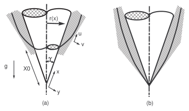
Figure 1: (a) Coordinate system for the boundary layer on a heated frustum of a cone, (b) full cone, $x_{0}=0$.

Consider an inverted cone with semi-angle $\gamma$ and take axes in the manner indicated in Fig. 1(a). The boundary layer develops over the heated frustum $x=x_{0}$.

The boundary layer equations for natural convection of Darcian fluid about a cone are Cheng and Pop :

$$\frac{\partial}{\partial x}(ru)+\frac{\partial}{\partial y}(rv)=0,$$ (2.1)

$$u=\frac{\rho_{\infty}\beta Kg\cos\gamma(T-T_{\infty})}{\mu},$$ (2.2)

$$u\frac{\partial T}{\partial x}+v\frac{\partial T}{\partial y}=\alpha\frac{\partial^{2}T}{\partial y^{2}}.$$

For a thin boundary layer, $r$ is obtained approximately $xsin(\gamma)$. Suppose that a power law of heat flux is prescribed on the frustum. Accordingly, the boundary conditions at infinity are:

$$u=0, ~{}T=T_{\infty},~{}~{}\text{if}~{}~{}y\rightarrow\infty$$ (2.3)

and at the wall are

$$v=0~{}~{}\text{if}~{}~{}y=0.$$

If the surface heat flux $q_{w}$ Cheng and Pop is prescribed, $q_{w}$ is obtained as

$$q_{w}={-k(\frac{\partial T}{\partial y}})_{y=0}=A(x-x_{0})^{\lambda},~{}~{}~{}~{}~{}x_{0}\leq x\leq\infty.$$

For the case of a full cone $(x_{0}=0,Fig.\ref{Fig.FullCone}(b))$ a similarity solution exists Cheng and Pop .

In the case of prescribed surface heat flux the similarity solution for the stream function $\psi$ and $T$ where

$$u=\frac{1}{r}\frac{\partial\psi}{\partial y},~{}~{}~{}v=-\frac{1}{r}\frac{\partial\psi}{\partial x}$$ (2.5)

is of the form Cheng and Pop :

$$\psi=\alpha r(Ra_{x})^{1/3}f(\eta),~{}~{}~{}~{}~{}~{}~{}~{}$$ (2.6)

$$T-T_{\infty}=\frac{q_{w}x}{k}(Ra_{x})^{-\frac{1}{3}}\theta(\eta),$$

$$\eta=\frac{y}{x}(Ra_{x})^{1/3},$$

where

$$Ra_{x}=\frac{\rho_{\infty}\beta gK\cos(\gamma)q_{w}x^{2}}{\mu\alpha k}$$ (2.7)

is the local Rayleigh number for the case of prescribed surface heat flux. The governing equations become

$$f^{\prime}=\theta,~{}~{}~{}~{}~{}~{}~{}~{}~{}~{}~{}~{}~{}~{}~{}~{}~{}~{}~{}~{}~{}~{}~{}~{}~{}~{}~{}~{}~{}~{}~{}~{}$$ (2.8)

$$\theta^{\prime\prime}+\frac{\lambda+5}{2}f\theta^{\prime}-\frac{2\lambda+1}{3}f^{\prime}\theta=0,$$

subjected to boundary conditions as:

$$f(0)=0,~{}~{}~{}\theta^{\prime}(0)=-1,~{}~{}~{}\theta(\infty)=0.$$ (2.9)

Finally from Eqs. (2.8) and (2.9) we have:

$$\begin{cases}ODE.\quad f^{\prime\prime\prime}+\left(\frac{\lambda+5}{2}\right)ff^{\prime\prime}-\left(\frac{2\lambda+1}{3}\right)(f^{\prime})^{2}=0,\cr B.C.\quad f(0)=0,\quad f^{\prime\prime}(0)=-1,\quad f^{\prime}(\infty)=0.\end{cases}$$ (2.10)

It is of interest to obtain the value of the local Nusselt number which is defined as Cheng and Pop :

$$Nu_{x}=\frac{q_{w}x}{k(T_{w}-T_{\infty})}.$$ (2.11)

From Eqs. (2.11), (2.6) and (2.7) it follows that the local Nusselt number which is interest to obtain given by:

$$Nu_{x}=Ra_{x}^{1/3}[-\theta(0)].$$ (2.12)

3 RBF Functions

Let $\mathbb{R}^{+}=\{x\in\mathbb{R},x\geq 0\}$ be the non-negative half-line and let $\phi:\mathbb{R}^{+}\to\mathbb{R}$ be a continuous function with $\phi(0)\geq 0$. A radial basis function on $\mathbb{R}^{d}$ is a function of the form

$$\phi(\|X-X_{i}\|)$$

where $X,~{}X_{i}\in\mathbb{R}^{d}$ and $\|.\|$ denotes the Euclidean distance between $X,~{}X_{i}$. If one chooses $N$ points $\{X_{i}\}_{i=1}^{N}$ in $\mathbb{R^{d}}$ then by custom

$$s(X)=\sum_{i=1}^{N}\lambda_{i}\phi(\|X-X_{i}\|);\quad\lambda_{i}\in\mathbb{R},$$

is called a radial basis function as well golberg .
In order to explain RBF methods briefly, suppose that the one-dimensional input data point set or the center set $x_{i}$ in the given domain $\Omega\subseteq\mathbb{R}$ is given. The center point is not necessarily structured, that is, it can have an arbitrary distribution. The arbitrary grid structure is one of the major differences between the RBF method and other global methods. Such a mesh-free grid structure yields high flexibility especially when the domain is irregular. In this work the uniform grid is used for RBF approximation.

3.1 Properties of RBF

With a radial function $\phi(r)$ and with data values $u_{i}$ given at the locations $x_{i}$, for $i=1,2,...,N$ the function

$$s(x)=\sum_{i=1}^{N}\lambda_{i}\phi_{i}(x)$$ (3.1)

where $r=r_{i}=\|x-x_{i}\|$ and $\phi_{i}(x)=\phi(\|x-x_{i}\|)$, interpolates the data if we choose the expansion coefficients $\lambda_{i}$ in such a way that $s(x_{j})=u_{j}$, for $j=1,2,...,N$ M.D.Buhmann 2000 ; Fasshauer.G.E.(2007) . The expansion coefficients $\lambda_{i}$ can therefore be obtained by solving the linear system $A\Lambda=U$, where:

$$A_{ij}=\phi(\|x_{j}-x_{i}\|),$$ (3.2)

$$\Lambda=[\lambda_{1},\lambda_{2},...,\lambda_{N}]^{T},$$ (3.3)

$$U=[u_{1},u_{2},\dots,u_{N}]^{T}.$$ (3.4)

All the infinitely smooth RBF choices listed in Table (1) will give coefficient matrices $A$ in (3.2) which are symmetric and nonsingular Powell , i.e. there is a unique interpolant of the form (3.1) no matter how the distinct data points are scattered in any number of space dimensions. In the cases of inverse quadratic, inverse multiquadric and GA the matrix $A$ is positive definite and, for multiquadric (MQ), it has one positive eigenvalue and the remaining ones are all negative Powell .
Interpolation using Conical splines and thin-plate splines (TPSs) can become singular in multidimensions Bengt Fornberg 2008 . However, low-degree polynomials can be added to the RBF interpolant to guarantee that the interpolation matrix is positive definite (a stronger condition than nonsingularity). For example, for the Conical RBF and the TPS in $d$ dimensions this becomes the case if we use as an interpolant $s(x)=\sum_{i=1}^{m}a_{i}p_{i}(x)+\sum_{i=1}^{N}\lambda_{i}\phi(\|x-x_{i}\|)$ together with the constraints $\sum_{j=1}^{N}\lambda_{j}p_{i}(x_{j})=0$, for $i=1,2,...,m$. Here $p_{i}(x)$ denotes a basis for polynomials of $\mathcal{P}^{d}_{q}$ in $\mathbf{R}^{d}$ ($\mathcal{P}^{d}_{q}$ denotes the space of d-variate polynomials of order not exceeding q) and $m=(q-1+d)!/(d!(q-1)!)$ Mehdi Dehghan Ali Shokri .

3.2 RBF Interpolation

One dimensional function $u(x)$ to be interpolated or approximated can be represented by an RBF as:

$$u(x)\approx s(x)=\sum_{i=1}^{N}\lambda_{i}\phi_{i}(x)=\Phi^{T}(x)\Lambda$$ (3.5)

where

$$\Phi^{T}(x)=[\phi_{1}(x),\phi_{2}(x),...,\phi_{N}(x)],$$ (3.6)

$$\Lambda=[\lambda_{1},\lambda_{2},...,\lambda_{N}]^{T},$$ (3.7)

$x$ is the input and $\lambda_{i}$s are the set of coefficients to be determined. By choosing $N$ interpolate nodes $(x_{j},j=1,2,...,N)$ in $\Omega\cup\partial\Omega$, the function $u(x)$ can be approximated in $\Omega\cup\partial\Omega$.

$$u_{j}=\sum_{i=1}^{N}\lambda_{i}\phi_{i}(x_{j}),\quad(j=1,2,...,N).$$ (3.8)

To brief discussion on coefficient matrix we define:

$$A\Lambda=U$$ (3.9)

where

$$U= [u_{1},u_{2},...,u_{N}]^{T},$$ (3.10)

$$A= [\Phi^{T}(x_{1}),\Phi^{T}(x_{2}),...,\Phi^{T}(x_{N})]^{T}$$

$$= \left(\begin{array}[]{cccc}\phi_{1}(x_{1})&\phi_{2}(x_{1})&\dots&\phi_{N}(x_{1})\\ \phi_{1}(x_{2})&\phi_{2}(x_{2})&\dots&\phi_{N}(x_{2})\\ \vdots&\vdots&\ddots&\vdots\\ \phi_{1}(x_{N})&\phi_{2}(x_{N})&\dots&\phi_{N}(x_{N})\\ \end{array}\right).$$ (3.15)

Note that $\phi_{i}(x_{j})=\phi(\|x_{i}-x_{j}\|)$ therefore $\phi_{i}(x_{j})=\phi_{j}(x_{i})$ consequently $A=A^{T}$.
The shape parameter $c$ which is shown in Table (1) affects both the accuracy of the approximation and the conditioning of the interpolation matrix S Sarra . In general, for a fixed number of $N$, smaller shape parameters produce the more accurate approximations, but also are associated with a poorly conditioned $A$. The condition number also grows with $N$ for fixed values of the shape parameter $c$. Many researchers (e.g.Carlson and Foley ; Rippa ) have attempted to develop algorithms for selecting optimal values of the shape parameter. The optimal choice of the shape parameter is still an open question. In practice it is most often selected by brute force. Recently, Fornberg et. al.B. Fornberg have developed a Contour-Padé algorithm which is capable of stably computing the RBF approximation for all $c>0$ S Sarra .
The following theorem about the convergence of RBF interpolation is discussed WuZM 2002 ; WuZM 1993 .

Theorem 3.1

assume ${x_{i}},(i=1,2,...,N)$ are N nodes in $\Omega$ which is convex, let

$$h=\max_{x\in\Omega}\min_{1\leq i\leq N}\|x-x_{i}\|_{2}$$

when $\hat{\phi}(\eta)<c(1+|\eta|)^{-(2l+d)}$ for any u(x) satisfies$\int{(\hat{u}(\eta))^{2}}/{\hat{\phi}(\eta)}d\eta<\infty$ we have

$$\|u^{N(\alpha)}-u^{(\alpha)}\|_{\infty}\leq{ch^{l-\alpha}}$$

where $\phi(x)$ is RBF and the constant $c$ depends on the RBF, d is space dimension, l and $\alpha$ are nonnegative integer. It can be seen that not only RBF itself but also its any order derivative has a good convergence.

3.3 Direct RBF for ODEs (DRBF)

In the direct method, the closed form DRBF approximating function (3.5) is first obtained from a set of training points, and its derivative of any order, e.g. $p$th order, can then be calculated in a straightforward manner by differentiating such a closed form DRBF as follows:

$$\frac{d^{k}s(x)}{dx^{k}}=\frac{d^{k}}{dx^{k}}(\sum_{i=1}^{N}\lambda_{i}\phi_{i}(x))=\sum_{i=1}^{N}\lambda_{i}\frac{d^{k}\phi_{i}(x)}{dx^{k}}=\sum_{i=1}^{N}\lambda_{i}G_{i}^{[k]}(x)$$ (3.16)

where

$$G_{i}^{[k]}(x)={d^{k}\phi_{i}(x)}/{dx^{k}},\qquad k=0,1,...,p.$$

Now we aim to apply the DRBF method for solving the ODEs in general form :

$$\begin{cases}F(x,u,u^{\prime},...,u^{(p-1)},u^{(p)})=0,&a\leq x\leq b,\cr u^{(i)}(e_{i})=\alpha_{i+1},&i=0,1,...,p-1,\end{cases}$$ (3.17)

where $e_{i}\in\{a,b\}$ and $u^{(i)}(x)=d^{i}u(x)/dx^{i}$, $F$ is known function and $\{\alpha_{i}\}_{i=1}^{p}$ are known constants. By substituting Eq. (3.5) in (3.17) and using Eq. (3.16) we have:

$$F(x,s,s^{\prime},...,s^{(p)})=F(x,\sum_{i=1}^{N}\lambda_{i}G_{i}^{[0]}(x),\sum_{i=1}^{N}\lambda{i}G_{i}^{[1]}(x),...,\sum_{i=1}^{N}\lambda_{i}G_{i}^{[p]}(x)).$$

Now, to obtain $\lambda_{i}$s $(i=1,2,...,N)$ we define the residual function:

$$Res(x)=F(x,s,s^{\prime},...,s^{(p)}).$$ (3.18)

The set of equations for obtaining the coefficients $\{\lambda_{i}\}_{i=1}^{N}$ come from equalizing Eq. (3.18) to zero at $N-p$ interpolate nodes $\{x_{j}\}_{j=1}^{N-p}$ plus $p$ boundary conditions:

$$\begin{cases}Res(x_{j})=0,&j=1,2,...,N-p,\cr\sum_{i=1}^{N}\lambda_{i}G_{i}^{[k]}(e_{i})=\alpha_{i+1},&k=0,1,...,p-1.\end{cases}$$ (3.19)

Since the direct approach is based on a differentiation process, all derivatives obtained here are very sensitive to noise arising from the interpolation of DRBFs from a set of discrete data points. Any noise here, even at the small level, will be badly magnified with an increase in the order of derivative N. Mai-Duy 2005 .

3.4 Indirect RBF for ODEs (IRBF)

In the indirect method, the formulation of the problem starts with the decomposition of the highest order derivative under consideration into RBFs. The obtained derivative expression is then integrated to yield expressions for lower order derivatives and finally for the original function itself. In contrast, the integration process, where each integral represents the area under the corresponding curve, is much less sensitive to noise. Based on this observation, it is expected that through the integration process, the approximating functions are much smoother and therefore have higher approximation power. Also To numerically explore tile IRBF methods with shape parameters for which the interpolation matrix is too poorly conditioned to use standard methods Fornberg and Wright . Let $p$ be the highest order of the derivative under consideration the boundary value ODEs in general form Eq. (3.17) when ($\exists k$ s.t. $e_{k}=b$) then we can define:

$$\frac{d^{p}\hat{s}(x)}{dx^{p}} =\sum_{i=1}^{N}\lambda_{i}\phi_{i}(x),$$ (3.20)

$$\frac{d^{p-1}\hat{s}(x)}{dx^{p-1}} =\int{\sum_{i=1}^{N}\lambda_{i}\phi_{i}(x)dx}=\sum_{i=1}^{N}\lambda_{i}\int{\phi_{i}(x)}dx=\sum_{i=1}^{N}\lambda_{i}h_{i}^{[p-1]}(x)+d_{1},$$

$$\vdots$$

$$\frac{d\hat{s}(x)}{dx} =\int{\sum_{i=1}^{N}\lambda_{i}h_{i}^{[2]}(x)}dx+d_{1}\frac{x^{p-2}}{(p-2)!}+d_{2}\frac{x^{p-3}}{(p-3)!}+...+d_{p-1}$$

$$=\sum_{i=1}^{N}\lambda_{i}h_{i}^{[1]}(x)+d_{1}\frac{x^{p-2}}{(p-2)!}+d_{2}\frac{x^{p-3}}{(p-3)!}+...+d_{p-1},$$

$$\hat{s}(x) =\int({\sum_{i=1}^{N}\lambda_{i}h_{i}^{[1]}(x)}+d_{1}\frac{x^{p-2}}{(p-2)!}+d_{2}\frac{x^{p-3}}{(p-3)!}+...+d_{p-1})dx$$

$$=\sum_{i=1}^{N}\lambda_{i}h_{i}^{[0]}(x)+d_{1}\frac{x^{p-1}}{(p-1)!}+d_{2}\frac{x^{p-2}}{(p-2)!}+...+d_{p-1}x+d_{p},$$

where

$$h_{i}^{[k]}(x)=\begin{cases}\int\phi_{i}(x)dx,&k=p-1,\cr\int h_{i}^{[k+1]}(x)dx,&k=0,1,...,p-2.\end{cases}$$ (3.21)

Substituting Eqs. (3.20) in (3.18) at $N$ interpolate nodes $\{x_{j}\}_{j=1}^{N}$ plus $p$ boundary conditions the set of coefficients $\{\lambda_{i}\}_{i=1}^{N}$ and $\{d_{j}\}_{j=1}^{p}$ is obtained as follow :

$$\begin{cases}Res(x_{j})=0,\quad&j=1,2,...,N,\cr\hat{s}^{(i)}(e_{i})=\alpha_{i+1},\quad&i=1,2,...,p.\end{cases}$$

4 Solving the model

Consider governing equation of fluid flow and heat transfer of full cone embedded in porous medium that is expressed by Eq. (2.10) for prescribed surface heat flux.

In the first step of our analysis, we approximate $f(\eta)$ for solving the model by DRBF:

$$f(\eta)\simeq s(\eta) =\sum_{i=1}^{N}\lambda_{i}\phi_{i}(\eta),$$ (4.1)

and $f^{\prime\prime\prime}(\eta)$ for solving the model by IRBF:

$$f^{\prime\prime\prime}(\eta)\simeq\frac{d^{3}}{d\eta^{3}}\hat{s}(\eta) =\sum_{i=1}^{N}\lambda_{i}\phi_{i}(\eta).$$ (4.2)

The general form of problem appear to:

$$\begin{cases}F_{\lambda}(\eta,f,f^{\prime},f^{\prime\prime},f^{\prime\prime\prime})=0,\cr f(0)=0,\ f^{\prime\prime}(0)=-1,\ f^{\prime}(\infty)=0.\end{cases}$$ (4.3)

To solve this problem we define residual function:

$$Res(\eta)=F_{\lambda}(\eta,s,s^{\prime},s^{\prime\prime},s^{\prime\prime\prime});\quad for\ DRBF,$$ (4.4)

$$Res(\eta)=F_{\lambda}(\eta,\hat{s},\hat{s}^{\prime},\hat{s}^{\prime\prime},\hat{s}^{\prime\prime\prime});\quad for\ IRBF.$$ (4.5)

The unknown coefficients $\{\lambda_{i}\}_{i=1}^{N}$ come from equalizing $Res(\eta)$ to zero at $N$ interpolate nodes $\eta_{i}$ from Uniform distribution between $0$ and $\eta_{\infty}$ which we set $9/2$ for this problem.

4.1 Solving the model by DRBF

In the first step of solving, $\phi_{i}(\eta)$ is set by inverse multiquadric function which is shown in Table (1). Now, the residual function is constructed by substituting Eq. (4.1) in Eq. (4.4):

$$Res(\eta) =\sum_{i=1}^{N}\lambda_{i}\phi_{i}^{{}^{\prime\prime\prime}}(\eta)+(\frac{\lambda+5}{2})(\sum_{i=1}^{N}\lambda_{i}\phi_{i}(\eta))(\sum_{i=1}^{N}\lambda_{i}\phi_{i}^{{}^{\prime\prime}}(\eta))-(\frac{2\lambda+1}{3})(\sum_{i=1}^{N}\lambda_{i}\phi_{i}^{{}^{\prime}}(\eta))^{2}.$$

By using $N-2$ interpolate nodes $\{\eta_{j}\}_{j=1}^{N-2}$ plus two boundary conditions of Eq. (4.3) $(f(0)=0,f^{\prime\prime}(0)=-1)$, the set of equations can be solved, consequently the coefficients $\{\lambda_{i}\}_{i=1}^{N}$ will be obtained:

$$\begin{cases}Res(\eta_{j})=0,&\quad j=1,2,...,N-2,\cr\sum_{i=1}^{N}\lambda_{i}\phi_{i}(0)=0,\cr\sum_{i=1}^{N}\lambda_{i}\phi_{i}^{\prime\prime}(0)=-1.\cr\end{cases}$$

Take into account $\phi^{\prime}_{i}(\infty)=0$, for $i=1,2,...,N$ the infinity boundary condition ($f^{\prime}(\infty)=0$) is already satisfied.
Table (2) show the $f^{\prime}(\eta)$ for some $\lambda$ in comparison with solutions of Sohouli.Famouri . Also $f^{\prime}(\eta)$ for two selected $\lambda=1/4$ and $3/4$ are showed in Table (3) in comparison with Runge-Kutta solution is obtained by the MATLAB software command ODE45 which is used and applied by the authors in ref. Sohouli.Famouri . Absolute errors show that DRBF give us approximate solution with a high degree of accuracy with a small $N$. The resulting graph of Eq. (2.10) is shown in Figure (2).

4.2 Solving the model by IRBF

In the first of solving $\phi_{i}(\eta)$ is set by multiquadric function which is shown in Table (1). Now, the residual function is constructed by substituting Eq. (4.2) in Eq. (4.5) and using Eq. (3.20):

$$Res(\eta) =\sum_{i=1}^{N}\lambda_{i}\phi_{i}(\eta)+(\frac{\lambda+5}{2})\sum_{i=1}^{N}\lambda_{i}\int\int\int\phi_{i}(\eta)d\eta\sum_{i=1}^{N}\lambda_{i}\int\phi_{i}(\eta)d\eta$$

$$-(\frac{2\lambda+1}{3})(\sum_{i=1}^{N}\lambda_{i}\int\int\phi_{i}({\eta})d\eta)^{2}$$

$$=\sum_{i=1}^{N}\lambda_{i}\phi_{i}(\eta)+(\frac{\lambda+5}{2})(\sum_{i=1}^{N}\lambda_{i}h_{i}^{[0]}(\eta)+\frac{d_{1}\eta^{2}}{2}+d_{2}\eta+d_{3})(\sum_{i=1}^{N}\lambda_{i}h_{i}^{[2]}(\eta)+d_{1})$$

$$-(\frac{2\lambda+1}{3})(\sum_{i=1}^{N}\lambda_{i}h_{i}^{[1]}(\eta)+d_{1}\eta+d_{2})^{2}.$$

By using $N$ interpolate nodes $\{\eta_{j}\}_{j=1}^{N}$ plus three boundary conditions of Eq. (4.3) the set of equations can be solved, consequently the coefficients $\{\lambda_{i}\}_{i=1}^{N}$ and $\{d_{i}\}_{i=1}^{3}$ will be obtained. In this method we put $\eta_{\infty}$ instead of infinity condition:

$$\begin{cases}Res(\eta_{j})=0,&\quad j=1,2,...,N,\cr\sum_{i=1}^{N}\lambda_{i}h_{i}^{[0]}(0)+d_{3}=0,\cr\sum_{i=1}^{N}\lambda_{i}h_{i}^{[2]}(0)+d_{1}=-1,\cr\sum_{i=1}^{N}\lambda_{i}h_{i}^{[1]}(\eta_{\infty})d_{1}\eta_{\infty}+d_{2}=0.\end{cases}$$

Table (4) shows the $f^{\prime}(\eta)$ for some $\lambda$ in comparison with solutions of Sohouli.Famouri . Also $f^{\prime}(\eta)$ for two selected $\lambda=1/4$ and $3/4$ are showed in Table (5) in comparison with Runge-Kutta solution is obtained by the MATLAB software command ODE45 which is used and applied by the authors in ref. Sohouli.Famouri . Absolute errors show that IRBF give us approximate solution with a high degree of accuracy with a small $N$. The resulting graph of Eq. (2.10) is shown in Figure (3). A graph in figures (4) for $\lambda=2/3$ show $\|Res\|^{2}$ for some $N$. Table (6) shows $\|Res\|^{2}$ for some $N$ and $\lambda$.
Comparison between DRBF solution in Table (3) with $N=12$ and IRBF solution in Table (5) with $N=10$ for $f^{\prime}(\eta)$ show that the convergence of the IRBF method is faster, because of using less numbers of collocation points.

5 Conclusion

In this paper we made a comparison between the two common collocation approaches based on radial basis functions namely DRBF and IRBF methods on natural convection equation about an inverted heated cone embedded in a porous medium of infinite extent which are of great importance in the design of canisters for nuclear wastes disposal. These functions are proposed to provide an effective but simple way to improve the convergence of the solution by collocation method. The direct approach (DRBF) is based on a differentiation process, all derivatives are very sensitive to noise arising from the interpolation of DRBFs from a set of discrete data points. Any noise, even at the small level, will be bad magnified with an increase in the order of derivative. The indirect technique (IRBF) which is based on integration process, each integral represents the area under the corresponding curve, is much less sensitive to noise. Based on this observation, it is expected that through the integration process, the approximating functions are much smoother and therefore have higher approximation power. Additionally, through the comparison with other methods such as HAM we show that the RBFs methods have good reliability and efficiency. Also high convergence rates and good accuracy are obtained with the proposed method using relatively low numbers of data points.

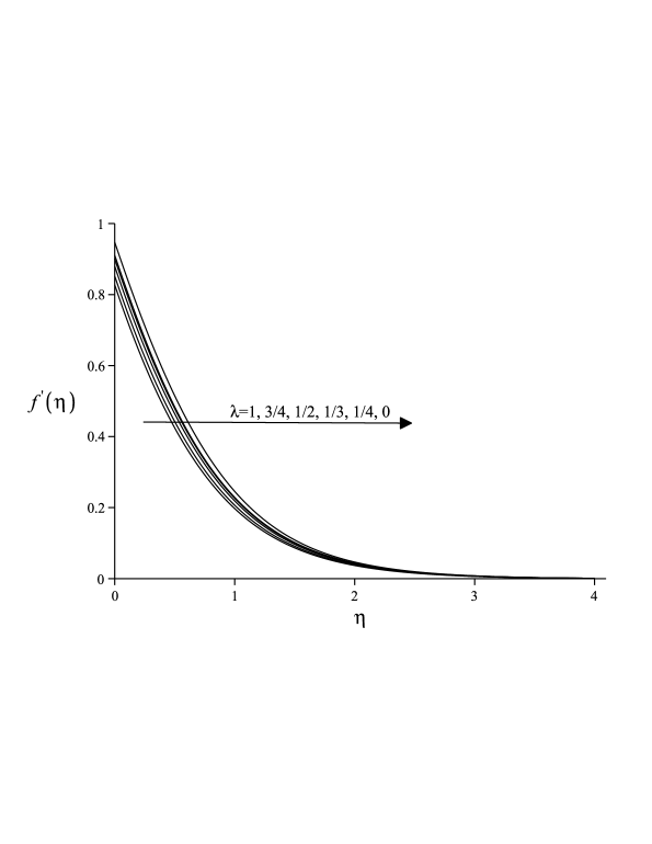
Figure 2: DRBF approximation of $f^{\prime}(\eta)$ for different values $\lambda=0,~{}1/4,~{}1/3,~{}1/2,~{}3/4$ and $1$

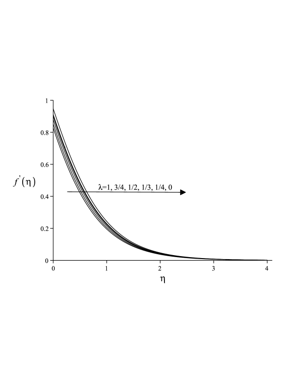
Figure 3: IRBF approximation of $f^{\prime}(\eta)$ for different values $\lambda=0,~{}1/4,~{}1/3,~{}1/2,~{}3/4$ and $1$

Figure 4: $\|Res\|^{2}$ for $\lambda=2/3$

Nomenclature
$A$	prescribed constant
$f$	similarity function for stream function temperature
$g$	acceleration due to gravity parameter
$K$	permeability of the fluid-saturated porous medium
$Nu_{x}$	local Nusselt number
$q_{w}$	surface heat flux fluid-saturated porous medium
$r$	local radius of the cone fluid
$Ra_{x}$	local Raleigh number
$T$	temperature
$T_{\infty}$	ambient temperature
$u,v$	velocity vector along x,y axis
$x,y$	Cartesian coordinate system
$x_{0}$	distance of start point of cone from the vertex
Greek symbols
$\alpha$	thermal diffusivity the fluid-saturated porous medium
$\beta$	expansion coefficient of the fluid
$\eta$	independent dimensionless
$\theta$	similarity function for
$\lambda$	prescribed constants
$\mu$	viscosity of the fluid
$\rho_{\infty}$	density of the fluid at infinity
$\psi$	stream function

Table 1: Some well–known functions that generate RBFs $(r=\|x-x_{i}\|=r_{i}),~{}c>0$

Name of functions	Definition
Multiquadrics (MQ)	$\sqrt{r^{2}+c^{2}}$
Inverse multiquadrics (IMQ)	$1/(\sqrt{r^{2}+c^{2}})$
Thin plate (polyharmonic)Splines (TPS)	$(-1)^{k+1}r^{2k}log(r)$
Conical splines	$r^{2k+1}$
Gaussian (GA)	$exp(-cr^{2})$
Exponential spline	$exp(-cr)$

Table 2: A comparison between solutions obtained by Sohouli.Famouri and the DRBF method for $f^{\prime}(0)$

	Runge-Kutta	DRBF method				Other methods
$\lambda$	SolutionSohouli.Famouri	N	c	DRBF	Error with RK	HAMSohouli.Famouri
$0$	$0.94760$	$10$	$3.46543$	$0.94750$	$0.0001$	$0.94783$
$1/4$	$0.91130$	$12$	$3.943$	$0.91086$	$0.00044$	$0.91119$
$1/3$	$0.90030$	$10$	$4.9665$	$0.90038$	$0.0008$	$0.90103$
$1/2$	$0.87980$	$10$	$5.36$	$0.87981$	$0.00001$	$0.87964$
$3/4$	$0.85220$	$12$	$5.23$	$0.85227$	$0.00007$	$0.85242$
$1$	$0.82760$	$10$	$5.89$	$0.82737$	$0.00023$	$0.82726$

Table 3: Comparison between DRBF solution and Runge-Kutta solution for $f^{\prime}(\eta)$ for $\lambda=1/4$ and $\lambda=3/4$ with $N=12$

	$\lambda=1/4,f^{\prime}(\eta)$			$\lambda=3/4,f^{\prime}(\eta)$
	DRBF	Runge-Kutta	Error	DRBF	Runge-Kutta	Error
$\eta$	Solution	SolutionSohouli.Famouri	with RK	Solution	SolutionSohouli.Famouri	with RK
$0$	$0.910886$	$0.911295$	$0.000409$	$0.852268$	$0.852193$	$0.000075$
$0.1$	$0.813122$	$0.813604$	$0.000482$	$0.755678$	$0.755377$	$0.000301$
$0.2$	$0.720720$	$0.721351$	$0.000631$	$0.666229$	$0.665448$	$0.000781$
$0.3$	$0.634656$	$0.635531$	$0.000875$	$0.584176$	$0.582985$	$0.001191$
$0.4$	$0.555601$	$0.556661$	$0.001061$	$0.509628$	$0.508141$	$0.001487$
$0.5$	$0.483877$	$0.484997$	$0.001120$	$0.442519$	$0.440849$	$0.001670$
$0.6$	$0.419467$	$0.420587$	$0.001120$	$0.382620$	$0.380907$	$0.001713$
$0.7$	$0.362196$	$0.363276$	$0.001080$	$0.329539$	$0.327973$	$0.001566$
$0.8$	$0.311655$	$0.312677$	$0.001022$	$0.282878$	$0.281536$	$0.001342$
$0.9$	$0.267358$	$0.268264$	$0.000906$	$0.242076$	$0.241013$	$0.001043$
$1$	$0.228756$	$0.229508$	$0.000752$	$0.206652$	$0.205832$	$0.000820$
$1.1$	$0.195268$	$0.195878$	$0.000610$	$0.176015$	$0.175434$	$0.000581$
$1.2$	$0.166342$	$0.166847$	$0.000505$	$0.149653$	$0.149275$	$0.000378$
$1.3$	$0.141450$	$0.141837$	$0.000387$	$0.127026$	$0.126821$	$0.000205$
$1.4$	$0.120090$	$0.120362$	$0.000272$	$0.107681$	$0.107596$	$0.000085$
$1.5$	$0.101811$	$0.102025$	$0.000214$	$0.091167$	$0.091196$	$0.000029$

Table 4: A comparison between solutions obtained by Sohouli.Famouri and the IRBF method for $f^{\prime}(0)$

	Runge-Kutta	IRBF method				Other methods
$\lambda$	SolutionSohouli.Famouri	N	c	IRBF	Error with RK	HAMSohouli.Famouri
$0$	$0.94760$	$10$	$1.860$	$0.94758$	$0.00002$	$0.94783$
$1/4$	$0.91130$	$10$	$2.005$	$0.91128$	$0.00002$	$0.91119$
$1/3$	$0.90030$	$10$	$2.050$	$0.90030$	$0.00000$	$0.90103$
$1/2$	$0.87980$	$10$	$2.150$	$0.87979$	$0.00001$	$0.87964$
$3/4$	$0.85220$	$10$	$2.418$	$0.85206$	$0.00014$	$0.85242$
$1$	$0.82760$	$10$	$2.380$	$0.82762$	$0.00002$	$0.82726$

Table 5: Comparison between IRBF solution and Runge-Kutta solution for $f^{\prime}(\eta)$ for $\lambda=1/4$ and $\lambda=3/4$ with $N=10$

	$\lambda=1/4,f^{\prime}(\eta)$			$\lambda=3/4,f^{\prime}(\eta)$
	IRBF	Runge-Kutta	Error	IRBF	Runge-Kutta	Error
$\eta$	Solution	SolutionSohouli.Famouri	with RK	Solution	SolutionSohouli.Famouri	with RK
$0$	$0.911278$	$0.911295$	$0.000017$	$0.852059$	$0.852193$	$0.000134$
$0.1$	$0.813594$	$0.813604$	$0.000010$	$0.755254$	$0.755377$	$0.000123$
$0.2$	$0.721302$	$0.721351$	$0.000049$	$0.665278$	$0.665448$	$0.000170$
$0.3$	$0.635394$	$0.635531$	$0.000137$	$0.582736$	$0.582985$	$0.000249$
$0.4$	$0.556440$	$0.556661$	$0.000221$	$0.507827$	$0.508141$	$0.000314$
$0.5$	$0.484753$	$0.484997$	$0.000244$	$0.440510$	$0.440849$	$0.000339$
$0.6$	$0.420334$	$0.420587$	$0.000253$	$0.380599$	$0.380907$	$0.000308$
$0.7$	$0.362989$	$0.363276$	$0.000287$	$0.327647$	$0.327973$	$0.000326$
$0.8$	$0.312347$	$0.312677$	$0.000330$	$0.281184$	$0.281536$	$0.000352$
$0.9$	$0.267934$	$0.268264$	$0.000330$	$0.240696$	$0.241013$	$0.000317$
$1$	$0.229197$	$0.229508$	$0.000311$	$0.205482$	$0.205832$	$0.000350$
$1.1$	$0.195584$	$0.195878$	$0.000294$	$0.175053$	$0.175434$	$0.000381$
$1.2$	$0.166546$	$0.166847$	$0.000301$	$0.148891$	$0.149275$	$0.000384$
$1.3$	$0.141548$	$0.141837$	$0.000289$	$0.126408$	$0.126821$	$0.000413$
$1.4$	$0.120107$	$0.120362$	$0.000255$	$0.107158$	$0.107596$	$0.000438$
$1.5$	$0.101771$	$0.102025$	$0.000254$	$0.090757$	$0.091196$	$0.000439$
$2$	$0.043769$	$0.043951$	$0.000182$	$0.038887$	$0.039223$	$0.000336$
$2.5$	$0.018310$	$0.018546$	$0.000236$	$0.016225$	$0.016574$	$0.000349$
$3$	$0.007391$	$0.007610$	$0.000219$	$0.006433$	$0.006832$	$0.000399$
$3.5$	$0.002716$	$0.002953$	$0.000237$	$0.002255$	$0.002668$	$0.000413$
$4$	$0.000719$	$0.000962$	$0.000243$	$0.000445$	$0.000913$	$0.000468$
$4.5$	$0.000010$	$0.000123$	$0.000113$	$-0.00001$	$0.000237$	$0.000247$

Table 6: $\|Res\|^{2}$ for different $N$ and $\lambda$ by IRBF

$\lambda$	N=5	N=6	N=8	N=10	N=12	N=15
$0$	$1.161037$	$0.306257$	$0.016229$	$0.000108$	$0.77e-5$	$0.11e-7$
$1/4$	$0.851976$	$0.278068$	$0.018364$	$0.000363$	$0.52e-4$	$0.27e-6$
$1/3$	$0.770207$	$0.269714$	$0.018842$	$0.000494$	$0.24e-4$	$0.13e-5$
$1/2$	$0.637068$	$0.216095$	$0.016813$	$0.000587$	$0.83e-5$	$0.47e-6$
$3/4$	$0.469112$	$0.230425$	$0.020280$	$0.001051$	$0.15e-4$	$0.83e-6$
$1$	$0.355474$	$0.221336$	$0.020463$	$0.001077$	$0.31e-4$	$0.39e-6$

References

• (1) D.A. Nield, A. Bejan, Convection in Porous Media, third ed., Springer-Verlag, New York, (2006).
• (2) J.H. Merkin, Free convection boundary layers in a saturated porous medium with lateral mass flux, Int. J. Heat Mass Transfer, 21 (1978) 1499-1504.
• (3) J.H. Merkin, Free convection boundary layers on axisymmetric and two dimensional bodies of arbitrary shape in a saturated porous medium, Int. J. Heat Mass Transfer, 22 (1979) 1461-1462.
• (4) W.J. Minkowycz, P. Cheng, Local non-similar solutions for free convective flow with uniform lateral mass flux in a porous medium, Lett. Heat Mass Transfer, 9 (1982) 159-168.
• (5) W.J. Minkowycz, P. Cheng, F. Moalem, The effect of surface mass transfer on buoyancy induced Darcian flow adjacent to a horizontal heated surface, Int. Commun. Heat Mass Transfer, 12 (1985) 55-65.
• (6) P. Cheng, T.T. Le, I. Pop, Natural convection of a Darcian fluid about a cone, Int. Commun. Heat Mass Transfer, 12 (1985) 705-717.
• (7) I. Pop, P. Cheng, An integral solution for free convection of a Darcian fluid about a cone with curvature effects, Int. Commun. Heat Mass Transfer, 13 (1986) 433-438.
• (8) D.B. Ingham, I. Pop, Natural convection about a heated horizontal cylinder in a porous medium, J. Fluid Mech. 184 (1987) 157-181.
• (9) I. Pop, D.B. Ingham Convective heat transfer: mathematical and computational modeling of viscous fluids and porous media, Pergamon Press, Oxford, 2001.
• (10) K. Vafai, Handbook of porous media. Marcel Dekker, New York, 2000.
• (11) A. Bejan, K.R. Khair, Heat and mass transfer by natural convection in a porous medium, Int. J. Heat Mass Transfer, 28 (1985) 909-918.
• (12) A. Nakayama, M.A. Hossain, An integral treatment for combined heat and mass transfer by natural convection in a porous medium, Int. J. Heat Mass Transfer, 38 (1995) 761-765.
• (13) K.A. Yih, Coupled heat and mass transfer by free convection over a truncated cone in porous media: VWT/VWC or VHF/VMF, Acta Mech. 137 (1999) 83-97.
• (14) K.A. Yih, Uniform transpiration effect on coupled heat and mass transfer in mixed convection about inclined surfaces in porous media : the entire regime, Acta Mech. 132 (1999) 229-240.
• (15) C.Y. Cheng, An integral approach for heat and mass transfer by natural convection from truncated cones in porous media with variable wall temperature and concentration, Int. Commun. Heat Mass Transfer, 27 (2000) 437-548.
• (16) C.Y. Cheng, Soret and Dufour effects on natural convection heat and mass transfer from a vertical cone in a porous medium, Int. Commun. Heat Mass Transfer, 36 (2009) 1020-1024.
• (17) S.U. Rahman, K. Mahgoub, A. Nafees, Natural Convective Mass Transfer from Upward Pointing Conical Surfaces in Porous Media, Chem. Eng. Commun. 194 (2007) 280-290.
• (18) I. Pop, T.Y. Na, Naturnal convection of a Darcian fluid about a wavy cone, Int. Commun. Heat Mass Transfer, 21 (1994) 891-899.
• (19) I. Pop, T.Y. Na, Natural convection over a frustum of a wavy cone in a porous medium, Mech. Res. Commun. 22 (1995) 181-190.
• (20) F. C. Lai and F. A. Kulacki, Coupled heat and mass transfer by natural convection from vertical surfaces in porous media, Int. J. Heat Mass Transfer, 34,4-5 (1991) 1189-1194.
• (21) A.R. Sohouli, M. Famouri, A. Kimiaeifar, G. Domairry, Application of homotopy analysis method for natural convection of Darcian fluid about a vertical full cone embedded in pours media prescribed surface heat flux, Commun. Nonlinear Sci. Numer. Simul. 15 (7) (2010) 1691-1699.
• (22) S. Abbasbandy, T. Hayat, Solution of the MHD Falkner-Skan flow by homotopy analysis method, Commun. Nonlinear Sci. Numer. Simul. 14 (9-10) (2009) 3591-3598.
• (23) S. Abbasbandy, Approximate solution for the nonlinear model of diffusion and reaction in porous catalysts by means of the homotopy analysis method, Chem. Eng. J. 136 (2008) 144-150.
• (24) K. Parand, M. Razzaghi, Rational Legendre approximation for solving some physical problems on semi-infinite intervals, Phys. Scr. 69 (2004) 353-357.
• (25) K. Parand, M. Dehghan, A. Pirkhedri, Sinc-collocation method for solving the Blasius equation, Phys. Lett. A, 373 (44) (2009) 4060-4065.
• (26) K. Parand, M. Dehghan, A.R. Rezaei, S.M. Ghaderi.An approximational algorithm for the solution of the nonlinear Lane-Emden type equations arising in astrophysics using Hermite functions collocation method, Comput. Phys. Commun. 2010; DOI:10.1016/j.cpc.2010.02.018.
• (27) K. Parand, A.R. Rezaei, S.M. Ghaderi, An approximate solution of the MHD Falkner-Skan flow by Hermite functions pseudospectral method, Commun. Nonlinear Sci. Numer. Simul. 2010; Doi:10.1016/j.cnsns.2010.03.022.
• (28) S. Abbasbandy, E. Shivanian, Exact analytical solution of a nonlinear equation arising in heat transfer, Phys. Lett. A, 374 (4) (2010) 567-574.
• (29) N. Mai-Duy, Solving high order ordinary differential equations with radial basis function networks, Int. J. Numer. Meth. Engng. 62 (6) (2005) 824-852.
• (30) E.J. Kansa, Multiquadrics-A scattered data approximation scheme with applications to computational fluiddynamics II. Solutions to parabolic, hyperbolic and elliptic partial differential equations, Comput. Math. Appl. 19 (8,9) (1990) 147-161.
• (31) M. Zerroukat, H. Power, C.S. Chen, A numerical method for heat transfer problems using collocation and radial basis functions, Int. J. Numer. Meth. Engng. 42 (1998) 1263-1278.
• (32) N. Mai-Duy, T. Tran-Cong, Numerical solution of differential equations using multiquadric radial basis function networks, Neural Netw. 14(2)(2001) 185-199.
• (33) N. Mai-Duy, T. Tran-Cong, Numerical solution of Navier Stokes equations using multiquadric radial basis function networks, Int. J. Numer. Meth Fluids, 37 (2001) 65-86.
• (34) B. Fornberg, Comparisons between pseudospectral and radial basis function derivative approximations, IMA J. Numer. Anal. 30 (1) (2008) 149-172.
• (35) N. Mai-Duy, T. Tran-Cong, Approximation of function and its derivatives using radial basis function network methods, Appl. Math. Modelling, 27 (2003) 197-220.
• (36) M.A. Golberg, C.S. Chen, H. Bowman, Some recent results and proposals for the use of radial basis functions in the BEM, Eng. Anal. Bound. Elem. 23 (4) (1999) 285-296.
• (37) M.D. Buhmann, Radial basis functions, Cambridge University Press, Cambridge, 2003.
• (38) G.E. Fasshauer, Meshfree Approximation Methods with Matlab, World Scientific Publishing, Singapore, (2007).
• (39) M.J.D. Powell, The theory of radial basis function approximation in 1990, Advances in Numerical Analysis, Clarendon, Oxford, (1992).
• (40) M. Dehghan, A. Shokri, A meshless method for numerical solution of the one-dimensional wave equation with an integral condition using radial basis functions, Numer. Algo. 52(3) (2009) 461-477.
• (41) R.E. Carlson, T.A. Foley, The parameter $r^{2}$ in multiquadric interpolation, Comput. Math. Appl. 21 (9) (1991) 29-42.
• (42) S. Rippa, An algorithm for selecting a good parameter c in radial basis function interpolation, Adv. Comput. Math. 11 (1999) 193-210.
• (43) B. Fornberg, T. Dirscol, G. Wright, R. Charles, Observations on the behavior of radial basis function approximations near boundaries, Comput. Math. Appl. 43 (2002) 473-490.
• (44) S.A. Sarra, Adaptive radial basis function method for time dependent partial differential equations, Appl. Numer. Math. 54 (2005) 79-94.
• (45) Z.M. Wu, Radial basis function scattered data interpolation and the meshless method of numerical solution of PDEs, J. Eng. Math. 19 (2) (2002), pp. 1 12 [In Chinese].
• (46) Z.M. Wu, R. Schaback, Local error estimates for radial basis function interpolation of scattered data, IMA J. Numer. Anal. 13 (1993) 13-27.
• (47) B. Fornberg, G. Wright, Stable computation of multiquadric interpolants for all values of the shape parameter, Computers Math. Applic. 48 (5/6) (2004) 853-867.
Refer to caption