Nonlinear Kinetic Development of the Weibel Instability
and the generation of electrostatic coherent structures

Abstract

The nonlinear evolution of the Weibel instability driven by the anisotropy of the electron distribution function in a collisionless plasma is investigated in a spatially one-dimensional configuration with a Vlasov code in a two-dimensional velocity space. It is found that the electromagnetic fields generated by this instability cause a strong deformation of the electron distribution function in phase space, corresponding to highly filamented magnetic vortices. Eventually, these deformations lead to the generation of short wavelength Langmuir modes that form highly localized electrostatic structures corresponding to jumps of the electrostatic potential.

I Introduction

The generation of macroscopic magnetic fields in a plasma is a fundamental process that occurs in laboratory and astrophysical plasma configurations in a wide range of regimes of plasma collisionality. This process appears naturally in a plasma. In plasma dynamics the “mechanical” and “electrodynamic” degrees of freedom couple very efficiently allowing for a rapid transfer from mechanical to electrodynamic energy and vice versa, as exemplified by the the dynamo mechanism DYNREV which is responsible for the generation of the magnetic fields of the planets and of the stars.

Here we are interested in investigating the different physical mechanisms that can accompany the generation of magnetic fields in a collisionless plasma regime, i.e., under conditions that are very far from thermodynamic equilibrium, and in particular in the generation of longitudinal electric fields and of electrostatic potential jumps due to nonlinear effects and to the related modification of the electron distribution function in phase space that accompany the generation of the magnetic field.

We refer in particular to the basic mechanism identified more than half a century ago by Weibel WEIBEL where the magnetic field is generated by the development of an instability driven by the temperature anisotropy of the electron distribution function in a collisionless plasma. Later on, a systematic linear kinetic analysis of the instabilities at play in an anisotropic plasma, without an initial mean magnetic field, has been carried out in an electron-ion plasma kalman . We recall that other mechanisms of magnetic field generation can be at play in different collisionality regimes, as extensively reviewed in Ref. HAINES .

A rough physical model of the magnetic field generation can be formulated in terms of a “thermal” machine working between the two ’temperatures’, $T_{x}$ and $T_{y}$ which correspond to the two ’temperatures’ that characterize the electron distribution function: $T_{y}$ describes the distribution width in $v_{y}$ and $T_{x}<T_{y}$ the distribution width in $v_{x}$. In a highly collisional regime the two temperatures would be rapidly equalized by the effect of collisions. In a collisionless plasma regime work can be extracted from this ’temperature’ difference. That this work is associated with the generation of magnetic field, i.e. in other words that this work corresponds to the transformation of thermal energy into magnetic energy, can be guessed by means of a virtual displacement argument borrowed from the theory of the closely related current filamentation instabilityCFI . We imagine splitting at each point the electron distribution function into two parts, corresponding to positive and to negative values of $v_{y}$ respectively, and displacing them in the transverse plane with a virtual displacement of the form $\xi^{+}_{0x}\sin{(k_{x}x)}=-\xi^{-}_{0x}\sin{(k_{x}x)}$, where the upper indices refer to the populations with positive and with negative value of $v_{y}$, respectively. In this way opposite current densities along $y$ are formed in the plasma. These currents are modulated along $x$ and produce a magnetic field along $z$. Since opposite currents repel, the initial displacement is reinforced, the instability can develop and the magnetic field along $z$ can grow.

Actually, the nonlinear evolution of the Weibel instability is far richer, even when we focus our investigation on a simplified geometrical configuration where all quantities are assumed to depend only on $x$ and velocity space is reduced to the $v_{x}$-$v_{y}$ plane. In this context we recall that the restriction to such a 1D-2V configuration excludes, among other phenomena that can accompany the nonlinear evolution of the Weibel instability, the development of a secondary magnetic field line reconnection instability of the type discussed in Ref. CALIFANOR .

In the one dimensional configuration considered here, the development of the Weibel instability is accompanied by the generation of electric fields: an inductive electric field in the $y$ direction intrinsically related to the variation in time of $B_{z}$ and a longitudinal field along $x$. For the sake of clarity, we recall that in the case of the related current filamentation instability, where an effective anisotropy in velocity space arises from the presence of two counterstreaming electron beams CFI , the growth of a longitudinal electric field in a two dimensional spatial configuration is due to the onset of a primary two-stream instability with wave vector along the direction of the beams (i.e. along $y$ with the choice of axes considered here). On the contrary, in the present case, the growth of a longitudinal electric field can only occur as a secondary process produced by the development of the Weibel instability itself. We also note that the generation of a longitudinal field, orthogonal to the beam direction, during the nonlinear evolution of the current filamentation instability in a one dimensional configuration was discussed analyticallyPrandi ; SPIKES in terms of a two fluid, cold plasma description and shown to occur near wave breaking conditions due to the nonlinear coupling between the current filamentation instability and Langmuir waves.

In the present article we recover within a kinetic description the nonlinear generation of a longitudinal field, orthogonal to the direction of the perturbed current produced by the Weibel instability in its linear phase. Furthermore we show that the nonlinear time evolution of the electron distribution function in phase space, in the presence of the magnetic and inductive electric fields produced by the Weibel instability, is characterized by a mixing process that occurs mostly at the position along $x$ where the amplitude of the magnetic field is largest and by particle acceleration or deceleration that occurs mostly at the position along $x$ where the amplitude of the inductive electric field is largest. The combination of these processes leads to the formation of a highly non monotonic distribution function in velocity space that can further excite Langmuir waves resonantly. Eventually, the evolution of the longitudinal fields is found to lead to the formation of multipolar electrostatic structures characterized by a bi-polar or tri-polar electric field profile that are reminiscent of the ”isolated electrostatic structures” detected by satellites in-situ in the solar wind plasma, in the auroral regions and in the Earth magnetosphere and bow shock. These structures have a typical width of the order of a few tenth of a Debye length and are thought to propagate along the magnetic field lines at speeds smaller than the solar wind speed. The tri-polar structures are also known as double-layers and are accompanied by a net potential drop. They have recently been proposed as a possible candidate in order to account, through a sequence of such double layers, for the total potential difference from the solar corona to the Earth, as consistent with exospheric models (see the recent review sw and references therein).

II Governing Equations

We consider high frequency modes evolving on electron time scales defined by the inverse of plasma frequency in a collisionless plasma and describe the dynamics of the plasma using the Vlasov-Maxwell system of equations for the electron distribution function ${f}_{e}$ taking the ions to remain at rest. Thus in dimensionless units we write

$$\frac{\partial{f}_{e}}{\partial{t}}+\mathbf{v}.\frac{\partial{f}_{e}}{\partial{\mathbf{x}}}+(\mathbf{E}+\mathbf{v}\times\mathbf{B})\cdot\ \frac{\partial{f}_{e}}{\partial{\mathbf{v}}}=0,$$ (1)

where velocities are normalized to the speed of light and times to the inverse of the plasma frequency $\omega_{pe}$. Lengths are thus normalized to the electron skin depth $d_{e}=c/\omega_{pe}$.

We restrict ourselves to a 1D-2V configuration where all quantities depend on $x$ and time only, the particle velocities and the electric field have $x$-$y$ components and the magnetic field is along the $z$ axis, and write Maxwell’s equations in the form

$$\frac{\partial{B_{z}}}{\partial{t}}=-\frac{\partial{E_{y}}}{\partial{x}},\qquad-\frac{\partial{B_{z}}}{\partial{x}}=\frac{\partial{E_{y}}}{\partial{t}}+J_{y},\qquad\frac{\partial^{2}\phi}{\partial^{2}x}=-\rho,$$ (2)

where $\rho$ and $\mathbf{j}$ are the dimensionless charge and current densities and $\phi$ the dimensionless electrostatic potential.

The Vlasov equation (1) is integrated in the phase space $(x,v_{x},v_{y})$ with periodic boundary conditions along the $x$ direction. For a description of the adopted code see Ref. Mang . We take the following initial condition

$$f_{e}(x,v_{x},v_{y},t=0)=f_{M}(v_{x},v_{y})[1+\epsilon\sum^{N}_{n=1}\ \cos(k_{n}x+\phi_{n}))];\hskip 14.22636ptk_{n}=2\pi n/L_{x}.$$ (3)

Here $L_{x}$ is the length of the simulation domain in the $x$ direction, $\epsilon$ is the perturbation amplitude varied in the range $10^{-6}\leq\epsilon\leq 10^{-4}$ and $f_{M}(v)$ is a two-temperature Maxwellian distribution given by

$$f_{M}(v_{x},v_{y})=\frac{n_{e}}{\pi\sqrt{T_{x}T_{y}}}\\ exp\Big{(}-\frac{v_{x}^{2}}{T_{x}}-\frac{v_{y}^{2}}{T_{y}}\Big{)},$$ (4)

with $T_{x}=4\cdot 10^{-4}$ corresponding to a plasma with a non-relativistic temperature, $T_{y}/T_{x}=12$ and $\phi_{n}$ are random phases. At $t=0$ we also introduce a perturbation on the magnetic field:

$$B_{z}=a_{i}\sum^{N}_{n=1}\ [\cos(k_{n}x+\psi_{n})],$$ (5)

where $a_{i}$ is the initial field amplitude for each wave and $\psi_{n}$ are random phases. We take $a_{i}=10^{-4}$ and $N=200$ in both Eqs. (3) and (5). We note the initial conditions with random initial amplitudes of the density and magnetic and electric field have been also used without any significative qualitative and quantitative change in the results.

We consider a field free plasma, hence $<B_{z}>=0$ at $t=0$. The computational velocity phase space is given by $[-v_{x}^{max},v_{x}^{max}]~{}\times~{}[-v_{y}^{max},v_{y}^{max}]$. We take $v_{x}^{max}=0.1$ and $v_{y}^{max}=0.27$ since the system is characterized by an initial temperature anisotropy $T_{y}>T_{x}$. However, the distribution function will spontaneously evolve towards a more isotropic configuration by reducing its width in the $v_{y}$ direction and by generating small scale filamentary structures with the same characteristic size in both directions. Therefore, we take a larger number of points in the $v_{y}$ direction in order to reduce the difference between the resolution in the two directions. For computational reasons (i.e. not to increase the total number of grid points too much), a good compromise is $N_{v_{x}}=281$ and $N_{v_{y}}=121$. The time step is $\Delta t=0.005\omega_{pe}^{-1}$. The evolution of the system is investigated up to $t=500\,\omega_{pe}^{-1}$. The length of the spatial simulation domain is $L_{x}=6\pi d_{e}$. The space discretization along $x$ is $dx=0.03\,d_{e}$, where $d_{e}$ is the electron skin depth, corresponding to $N_{x}=600$ grid points in the $x$ direction. This allows us to account for phenomena that occur on small spatial scales that are larger than, but of the order of, the electron Debye scale $\lambda_{D}=0.02\,d_{e}$.

III Onset of the Weibel instability and early nonlinear phase

Figure 1: Left frame: amplitude of the Fourier components of the magnetic field $B_{z,k}$ at $t=300$ vs. $k$. Right frame: time evolution of the Fourier components of the most unstable $k=k_{max}=1$ magnetic and inductive electric field mode, $B_{z,k=1}$ and $E_{y,k=1}$, solid and dashed line respectively, and of the most unstable $k=2.3$ longitudinal electric field $E_{x,k=2.3}$ (dotted line). The dash-three dotted line represents the growth rate of the magnetic field.

Figure 2: Growth of $k=1,2,2.3$ Fourier components of the longitudinal field $E_{x,k}$, dashed, dotted and solid line, respectively.

The onset and the linear growth of the Weibel instability up to the beginning of its saturation phase is shown in Fig. 1, as obtained from the numerical integration of the Vlasov equation described above. In the left frame the Fourier amplitude of the magnetic field $B_{z,k}$ at $t=300$ is shown vs. $k$ (note that only a part of the interval in $k$ is shown). We see that the modes in the range $0.3\leq k\leq 1.5$ have grown significantly with their maximum growth rate corresponding to $k=1$, i.e. in dimensional units to $k=d_{e}^{-1}$. In the right frame, the amplitude of the magnetic field $B_{z,k}$ vs. time is plotted for the most unstable mode, $k=1$ (solid line). After the initial transient phase the amplitude of the magnetic field grows exponentially, for $t\leq 270$ (linear phase), with growth rate $\gamma_{max}\sim 0.04$ (see dash-three dotted line), consistent with the analytical results (see Ref. WEIBEL ).

The growth of the inductive electric field component $E_{y,k}$ associated to $B_{z,k}$ is shown in the same frame (dashed line) still for $k=1$ , together with the longitudinal field $E_{x,k}$ (dotted line) taken at $k=2.3$. We note the $E_{y,k}$ reaches its maximum value at the saturation time of $B_{z,k}$ and then starts to decrease. This is consistent with the fact that the ratio between the inductive electric field and the magnetic field generated by the Weibel instability scales with the instability growth rate so that, as soon as the Weibel instability saturates, the mode structure is dominated by the magnetic field. In this phase the longitudinal electric field $E_{x,k}$ arises because of the coupling between the Weibel instability and the Langmuir waves, as discussed within the fluid approximation in Ref. SPIKES , due to the electron density modulation induced by the spatial modulation of $B^{2}_{z,k}$, and thus grows in time at twice the growth rate of the magnetic field.

While the Fourier component of the longitudinal field shown in Fig. 1, right frame, corresponds to $k=2.3$, the spectrum in $k$ of the longitudinal field and of the density modulation is wider, as consistent with the fact that the Weibel instability grows with very close growth rates in a relatively large range of values of $k$ around $k\sim 1$. As shown in Fig. 2, different Fourier components of the longitudinal field grow with nearly equal values of the growth rate. As a consequence, while the longitudinal field grows two times as fast as the magnetic field, its spatial structure contains additional wavelengths besides $\lambda/2=\pi$.

The frequency spectra of $B_{z,k}$ for fixed $k$, are shown in Fig. 3 for $k=1,8,10$. The spectral amplitude is largest for $k=1$ and in the low frequency part of the frequency spectrum corresponding to the Weibel instability. For larger values of $k$ the frequency spectra exhibit a weaker feature for large frequencies corresponding to low amplitude transverse electromagnetic waves propagating essentially at the speed of light ($\omega\sim k$ in dimensionless units).

Figure 3: Frequency spectra of the magnetic field component $B_{z,k}$ for $k=1,8,10$ (from left to right).

The frequency spectra of the longitudinal field $E_{x,k}$ at fixed $k$, are shown in Fig. 4 for $k=1,2,8$ and exhibit a clear peak at the electron plasma frequency. This peak appears to be less pronounced for larger values of $k$.

Figure 4: Frequency spectra of the longitudinal electric field component $E_{x,k}$ for $k=1,2,8$ (from left to right).

Additional numerical integrations of the Vlasov equation, not shown here, for different initial anisotropy ratios ($T_{y}/T_{x}=9$ and $T_{y}/T_{x}=4$) at constant $T_{x}$ indicate that, while the $k=1$ mode remains the most unstable electromagnetic mode, the spectrum of the excited modes becomes narrower with decreasing anisotropy, since higher $k$ modes grow less fast, as consistent with linear theory. This effect is also present in the spectrum of the longitudinal electric field $E_{x,k}$ in which case the value of $k$ corresponding to the maximum growth rate decreases as the anisotropy ratio is decreased. The maximum value of $B_{z}$, taken at the time when its growth is saturated, decreases with decreasing anisotropy ratio. Conversely, if $T_{x}$ is decreased at constant anisotropy ratio ($T_{y}/T_{x}=12$), the maximum value of $B_{z}$ is almost unchanged, while the value of $k$ corresponding to the maximum growth rate of the longitudinal electric field decreases from $k=2.3$ at $T_{x}=1$ to $k=2$ at $T_{x}=0.5$.

IV Phase space evolution in the advanced nonlinear phase

During the linear growth of the instability, the evolution of the electron distribution function in velocity space is characterized by a differential rotation in velocity space at the points where the absolute value $|B_{z}|$ of the magnetic field generated by the Weibel instability has a maximum and by a Y- shaped deformation with axis along $v_{y}$ at the points where the perturbed magnetic field vanishes which correspond to the points where the absolute value $|E_{y}|$ of the inductive electric field is largest. This behaviour is shown by the frames in the second row of Fig. 5. The rotation of the distribution function is clockwise or anti-clockwise depending on the sign of $B_{z}$ (labelled as $B_{max}$ and $B_{min}$ respectively in Fig. 5, while the Y-shaped deformation is turned upside down depending on the sign of $E_{y}$ (only one sign is shown in Fig. 5). As the Weibel instability enters its fully nonlinear phase the winding of the distribution function becomes tighter and the Y- deformation more marked until both features become ”multi-armed”, as shown by the last row in Fig. 5.

         

         

         

         

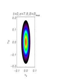
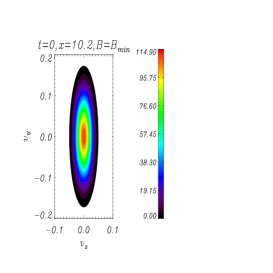
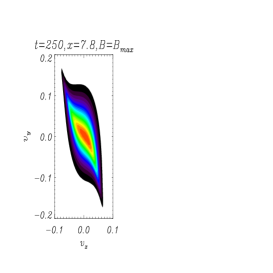
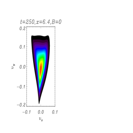
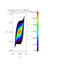
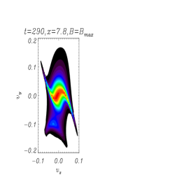
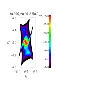
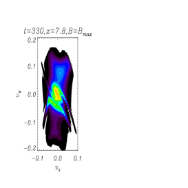
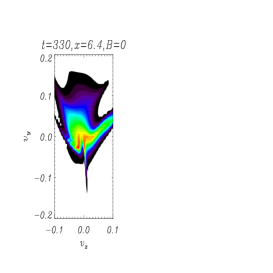
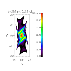
Figure 5: Time evolution of the electron distribution function with $t=0$(first row), $t=250$(second row), $t=290$(third row) and $t=330$(last row) at different positions along $x=7.8,6.4,10.2$ (from left to right). Red (blue) part is most (least) densely populated.

The winding of the distribution function and the formation of phase space vortices associated to the magnetic field $B_{z}(x)$ is also apparent from the contour plots of the distribution function at $t=340$ in the $x$-$v_{x}$ space shown in Fig. 6 for different values of $v_{y}$.

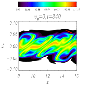
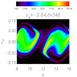
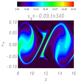
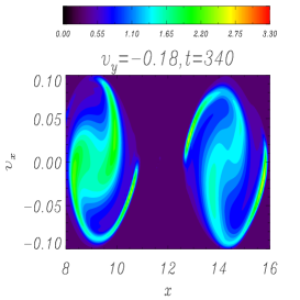
Figure 6: Contour plots of the distribution function in the $x$-$v_{x}$ space at $t=340$ for different values of $v_{y}$.

Disregarding for the moment the effect of the longitudinal electric field, this complex behaviour can be attributed to the combined effects of the magnetic field $B_{z}$, that deflects the electron orbits (where $|B_{z}|$ is largest and $E_{y}$ vanishes) and of the inductive electric field $E_{y}$ that accelerates or decelerates the electrons along $y$ (where $E_{y}$ is largest and $|B_{z}|$ vanishes). In order to visualize this combined effect of the instability fields on the plasma electrons a set of particle orbits have been computed by direct integration of the particle equation of motion in the electromagnetic fields obtained from the Vlasov integration (shown in Fig. 7 in ($x,t$) space).

For illustration a representative orbit is shown in Fig. 8. The particle is initialized at $x=10$ with $v_{0x}=0.01$ and $v_{0y}=0.05$ and moves straight until around $t=270$ the electromagnetic fields of the instability have grown significantly.

                 

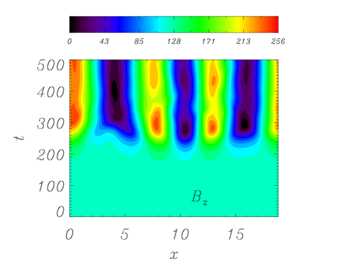
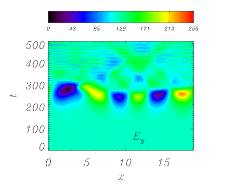
Figure 7: Contour plots showing the combined $x$-$t$ dependence of $B_{z}$ (left frame) and of $E_{y}$ (right frame).

Figure 8: Example of an electron orbit in the time evolving electromagnetic fields: particle velocities vs. time (top frames), particle trajectory (bottom left frame), particle kinetic energy vs. time (bottom right frame).

At this time this particle undergoes a net deceleration and its kinetic energy decreases while $v_{0x}$ and $v_{0y}$ become oscillatory. The same oscillatory behaviour is displayed by the particle kinetic energy. The particle trajectory becomes trapped along $x$ between two positions, separated by roughly half a wavelength of the dominant $k$ component of $B_{z}$, where the amplitude of the magnetic field is maximum ($B_{z}$ is negative near $x=10.5$ and positive near $x=12.5$).

As shown by the contour plots in Fig. 5 the electron distribution function becomes ”multi-armed” as the instability evolves. This implies that the distribution function develops steep positive slopes for velocities of the order of the electron thermal velocity along $x$ as shown in Fig. 9.

Figure 9: Electron distribution function at $x=7.8$ and $v_{y}=0$ vs. $v_{x}$ at $t=280,310,320$ (first three frames). Time evolution of the longitudinal electric field component $E_{x,k=25}$ (last frame). Electron distribution function at $t=0$ in the first frame with dashed lines.

Although these positive slopes evolve in time as the electron distribution function becomes increasingly twisted, they can give rise to a further excitation of Langmuir waves but with phase velocities much smaller than those of the Langmuir waves driven by the nonlinear coupling discussed in Sec. III. This new destabilizing process is shown in Fig. 9, last frame, where the time evolution of the longitudinal electric field component is shown versus time for $k=25$ which corresponds to a phase velocity along $x$ equal to $0.04$. Contrary to the components of the longitudinal field with large phase velocities shown in Fig. 2, in the initial phase this high-$k$, low phase velocity longitudinal field decays exponentially to noise level, as consistent with the strong Landau damping due to the initial Maxwellian shape of the electron distribution function. Later, around $t=280$, the non monotonic feature of the electron distribution function shown in the first frame in Fig. 9 makes the mode grow resonantly with a growth rate of the order of $\gamma=0.15$, i.e. faster than the low-$k$ modes produced by nonlinear density modulations. Eventually the mode reaches an amplitude that is smaller by approximately an order of magnitude than that of the low $k$ longitudinal modes.

A similar growth is also exhibited by longitudinal modes within a wide range of values of $k$ that extends towards larger values of $k$ and thus towards smaller phase velocities that resonate well inside the electron distribution function. The growth of these lower phase velocity modes starts somewhat earlier than that of the $k=25$ shown in Fig. 9 but reaches significantly lower final amplitudes.

This destabilization mechanism shows that in a collisionless plasma dominated by kinetic effects the nonlinear energy transfer between modes with different wave-number can occur nonlocally in $k$ space, with modes with higher values of $k$ being excited earlier than modes with comparatively lower values of $k$.

As mentioned before, smaller values of the magnetic field $B_{z}$ are found when smaller anisotropy ratios are considered. In this case the twisting of the electron distribution function is less pronounced and, consequently, the excitation of Langmuir waves with phase velocities resonating inside the electron distribution function is considerably weaker.

V Formation of electrostatic coherent structures

The wide spectrum of longitudinal modes that are excited by the phase space resonances discussed above leads to a highly structured electron density distribution $n_{e}$ along $x$, while the $k$ spectrum magnetic field generated by the Weibel instability is considerably narrower and $B_{z}$ remains spatially regular even at late times (see Fig. 7, left frame).

Figure 10: Plot of $B_{z}$and $E_{x}$, left and right frame versus $x$ at $t=468$.

This is also illustrated in Fig. 10 where we show the spatial profile of $B_{z}$ and $E_{x}$ versus $x$ at $t=468$. It is seen that the electric field, besides exhibiting a spatial modulation at roughly half the dominant magnetic field wavelength, has developed several narrow spikes, in particular a very narrow one at $x\sim 13.6$ (corresponding to a sharp minimum in the the electron density). In the one-dimensional configuration considered here, these spikes correspond to ”multi layer” electrostatic structures accompanied by a drop in the potential. A detailed analysis shows that these structures are not a true equilibrium between the electrostatic field and the pressure gradient, as is generally found for double layer coherent structures associated with phase space holes Ref. cal05 . However, since these structures survive on time scales of the order of several ion periods, we still define them as coherent electrostatic structures. The time evolution of the longitudinal electric field is shown in the first four frames in Fig. 11 vs. $x$ and in the last frames in Fig. 11 where $E_{x}$ at $x=13.6$ is plotted vs. $t$. A clear view of the formation of the electrostatic structures is given in Fig. 12 where we show the electrostatic field in the ($x,t$) plane. We see that after forming large scale structures on the magnetic (one-half) scale around $t=250$, slowly propagating small scales electrostatic multipolar structures are formed on the Debye length scale. As they propagate, these structures interact with each other leading to coalescence or to the formation of new structures with similar characteristics.   We observe that these structures do not form in the numerical simulations with smaller anisotropy ratios ($T_{y}/T_{x}=4$).

Figure 11: Top four frames: Plot of $E_{x}$ versus $x$ at $t=471,473,477,480$. Last two frames: Plot of $E_{x}$ versus $t$ at $x=13.6$

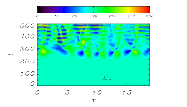
Figure 12: Contour plots in the ($x-t$) plane of the electrostatic field $E_{x}$.

Electrostatic features of this type are encountered under space conditions and were first observed almost thirty years ago in auroral regions in the form of dipolar electric structures as well as double layers Temerin . These ”large amplitude solitary structures” are in general observed with the electric field aligned with the mean magnetic field direction ergun . In the solar wind observations of dipolar structure have been reported starting from ten years ago in Ref. mangeney . From a theoretical point of view, there is no consensus about the origin of such structures. Accelerated particles, or beams, generated far away by some energetic events such as, for example, magnetic reconnection, are probably the best candidate for the energetic driver of the mechanism at the basis of the formation of multipolar structures matsumoto ; omura ; briandjgr . In this context, it is interesting to note that plasma temperature anisotropies, a typical feature expected in many regions in solar wind plasmas, may represent a possible source for their formation through a multi stage process that involves a complex evolution of the electron distribution function under the influence of the electromagnetic fields generated by the Weibel instability. A study of plasma electron temperature anisotropy in the presence of a weak, mean magnetic field (see gary1 for the linear analysis and gary2 for simulations) is in progress.

VI Conclusions

Pressure anisotropy is a common feature of laboratories and of space plasma and provides the free energy source for the development of the Weibel instability and the generation of a quasi static magnetic field. In this paper we have investigated the nonlinear evolution of the Weibel instability arising from the anisotropy of the electron distribution function in a collisionless plasma. We have adopted a two-dimensional velocity space Vlasov code in a simplified spatially one-dimensional configuration.

We have found that the instability causes a violent deformation of the electron distribution function in phase space leading to the generation of short wavelength Langmuir modes. This mechanism coexists with the ”fluid-like” generation of longer wavelength Langmuir modes due to the nonlinear modulation of the electron density. It corresponds to a non-local energy transport between modes in wave-number space. Eventually these short wavelength Langmuir modes lead to the formation of highly localized electrostatic structures. These structures correspond to potential jumps and are of interest for space observations.

References

-
(1)
G. K. Batchelor, Proc. R. Soc. London, A 201, 405 (1950);
A. P. Kazantsev, Sov. Phys. JETP, 26, 1031 (1968);
H. Moffatt, in Magnetic Field Generation in Electrically Conducting Fluids, (Cambridge University Press, Cambridge, 1978);
M. Meneguzzi, et al., Phys. Rev. Lett., 47, 1060 (1981);
Ya. B. Zeldovich et al., J. Fluid Mech., 144, 1 (1984). - (2) E.W. Weibel, Phys. Rev. Lett., 2, 83, (1959).
- (3) Kalman G. et al., Physics of Fluids 11, 1797 (1968)
- (4) M.G.Haines, Can. J. Phys., 64, 912, (1986) and references therein.
- (5) F. Califano et. al., Phys. Rev. E 58, 7837 (1998)
- (6) F. Califano, et al., Phys Rev Lett., 86, 5293 (2001)
- (7) F. Califano et. al., Phys. Rev., E 57, 7048 (1998)
- (8) F. Califano et. al., J. Plasma Phys, 60, 331 (1998)
- (9) C. Briand, Nonlin. Processes Geophys. 16, 319 (2009)
- (10) A. Mangeney et. al., J. Comp. Phys., 179, 495 (2002)
- (11) F. Califano et. al., Phys. Rev. Lett., 95, 245002 (2005)
- (12) M. Temerin et. al., Phys. Rev. Lett. 48, 1175 (1982)
- (13) R. Ergun et. al., Geophys. Res. Lett. 25, 2041 (1998)
- (14) A. Mangeney et. al., Ann. Geophys. 17, 307 (1999)
- (15) H. Matsumoto et. al., Geophys. Res. Lett. 21, 2915 (1994)
- (16) Y. Omura et al., J. Geophys. Res. 104, 14,627 (1999)
- (17) C. Briand et. al., J. Geophys. Res. 16, 319 (2009)
- (18) P. Gary et al., J. Geophys. Res. 111, A11224, (2006)
- (19) P. Gary et al., J. Geophys. Res. 105, 10,751, (2000)