A Tale of Two Electrons: Correlation at High Density

Abstract

We review our recent progress in the determination of the high-density correlation energy $E_{\rm c}$ in two-electron systems. Several two-electron systems are considered, such as the well known helium-like ions (helium), and the Hooke’s law atom (hookium). We also present results regarding two electrons on the surface of a sphere (spherium), and two electrons trapped in a spherical box (ballium). We also show that, in the large-dimension limit, the high-density correlation energy of two opposite-spin electrons interacting via a Coulomb potential is given by $E_{\rm c}\sim-1/(8D^{2})$ for any radial external potential $V(r)$, where $D$ is the dimensionality of the space. This result explains the similarity of $E_{\rm c}$ in the previous two-electron systems for $D=3$.

I Introduction

The Hartree-Fock (HF) approximation ignores the correlation between electrons, but gives roughly 99% of the total electronic energy Szabo . Moreover, it is often accurate for the prediction of molecular structure Helgaker , computationally cheap and can be applied to large systems, especially within local (linear-scaling) strategies White96 ; Schwegler96 ; Strain96 ; Burant96 ; Ochsenfeld98 ; Kitaura99 ; Komeiji03 ; Fedorov06 . To reduce the computational cost still further, various numerical techniques have been developed including, for example, density fitting (or resolution of the identity) Whitten73 ; Vahtras93 ; Dunlap77 ; Rendell94 ; Kendall97 ; Weigend02 , pseudospectral and Cholesky decomposition Martinez95 ; Friesner99 ; Beebe77 ; Roeggen86 ; Koch03 ; Aquilante07 ; Aquilante09 , dual basis methods Jurgens91 ; Wolinski03 ; Liang04 ; Steele06 ; Deng09 ; Deng10c , and both attenuation CASE96 ; CAP96 and resolution Dombroski96 ; RO08 ; Lag09 ; RRSE09 of the Coulomb operator.

Unfortunately, the part of the energy which the HF approximation ignores can have important chemical effects and this is particularly true when bonds are formed and/or broken. Consequently, realistic model chemistries require a satisfactory treatment of electronic correlation.

The concept of electron correlation was introduced by Wigner Wigner34 and defined as

$$E_{\rm c}=E-E_{\rm HF}$$ (1)

by Löwdin Lowdin59 , where $E$ is the exact non-relativistic energy. Feynman refered to $E_{\rm c}$ as the “stupidity energy” Feynman72 because of the difficulties associated with its characterization in large systems.

Even though it is a formidable challenge to determine the correlation energy accurately, even in simple systems, recent heroic calculations on the helium atom Nakashima07 ; Nakashima08a ; Nakashima08b ; Kurokawa08 have demonstrated how near-exact results can be found. Indeed, this elementary chemical system has been compared to the number $\pi$ by Charles Schwartz Schwartz06 : “For thousands of years mathematicians have enjoyed competing with one other to compute ever more digits of the number $\pi$. Among modern physicists, a close analogy is computation of the ground state energy of the helium atom, begun 75 years ago by E. A. Hylleraas.”

Although $E_{\rm c}$ in the helium atom is now known very accurately, certain correlation effects remain incompletely understood and, for example, even the Coulomb hole Coulson61 itself is more subtle than one might imagine. The primary effect of correlation is to decrease the likelihood of finding the two electrons close together and increase the probability of their being far apart. However, accurate calculations have revealed the existence of a secondary Coulomb hole, implying that correlation also brings distant electrons closer together Pearson09a . The same observation has been made in the H₂ molecule by Per et al. Per09 and it appears that secondary (or long-range) Coulomb holes may be ubiquitous in two-electron systems TEOCS10 .

In order to get benchmark results for the development of intracule functional theory (IFT) Gill06 ; Dumont07 ; Crittenden07a ; Crittenden07b ; Bernard08 ; Pearson09b ; Hollett10 , we have recently initiated an exhaustive study of two-electron systems BetheSalpeter . In the present Frontier Article, we review our recent progress in the determination of the correlation energy in various high-density two-electron systems: the helium-like ions (Sec. II.1), two electrons on the surface of a sphere (Sec. II.2), the Hooke’s law atom (Sec. II.3), and two electrons trapped in a spherical box (Sec. II.4).

It is reasonable to ask whether an understanding of the high-density regime is relevant to normal chemical systems but it turns out that most of the high-density behaviour of electrons is surprisingly similar to that at typical atomic and molecular electron densities. Much can be learned about the languid waltz of a pair of electrons in a covalent bond from their frenetic jig in the high-density limit. Moreover, it has led to an understanding of key systems, such as the uniform electron gas GellMann57 ; Vignale , which form the cornerstone of the popular local density approximation in solid-state physics ParrYang .

We also show (Sec. III) that, in the large-dimension limit, the high-density correlation energy of two electrons is given by a simple universal rule which is independent of the external confining potential. Just as one learns about interacting systems by studying non-interacting ones and then introducing the interaction perturbatively, one can understand our three-dimensional world by studying high-dimensional analogues and introducing dimension-reduction perturbatively.

In this study, we confine our attention to the ${}^{1}S$ ground states of two-electron systems. This allows us to ignore the spin coordinates and focus on the spatial part of the wave function. Atomic units are used throughout.

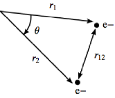
Figure 1: The basic coordinates of a two-electron system.

II High-density limit

For two electrons confined in a spherically-symmetric external potential $V(r)$, the Hamiltonian is

$$\hat{H}=-\frac{\nabla_{1}^{2}}{2}-\frac{\nabla_{2}^{2}}{2}+V(r_{1})+V(r_{2})+\frac{1}{r_{12}},$$ (2)

where the first two terms represent the kinetic energy of the electrons and $1/r_{12}=1/\left|\bm{r}_{1}-\bm{r}_{2}\right|$ is the Coulomb operator (Fig. 1). After a suitable scaling of the coordinates and energy EcLimit09 ; Proof , the Hamiltonian can be recast as

$$\hat{H}=-\frac{\nabla_{1}^{2}}{2}-\frac{\nabla_{2}^{2}}{2}+V(r_{1})+V(r_{2})+\frac{1}{Z}\frac{1}{r_{12}},$$ (3)

where $Z$ measures the confinement strength. Equation (3) is well poised for a perturbation treatment in which the zeroth- and first-order Hamiltonians are

$$\hat{H}^{(0)} =\hat{h}_{1}^{(0)}+\hat{h}_{2}^{(0)}, \hat{H}^{(1)} =\frac{1}{r_{12}},$$ (4)

and the one-electron Hamiltonian is given by

$$\hat{h}_{i}^{(0)}=-\frac{1}{2}\nabla_{i}^{2}+V(r_{i}).$$ (5)

The zeroth-order wave function satisfies the eigenequation

$$\hat{H}^{(0)}\Psi_{0}\left(r_{1},r_{2}\right)=E^{(0)}\Psi_{0}\left(r_{1},r_{2}\right),$$ (6)

and the zeroth- and first-order energies are

$$E^{(0)}=\left<\Psi_{0}\left|\hat{H}^{(0)}\right|\Psi_{0}\right>,$$ (7)

$$E^{(1)}=\left<\Psi_{0}\left|\hat{H}^{(1)}\right|\Psi_{0}\right>.$$ (8)

Following Hylleraas Hylleraas30 , we can use perturbation theory to expand both the exact Hylleraas30 and Hartree-Fock (HF) Linderberg61 energies as series in $1/Z$, yielding

$$E(Z,D,V)=E^{(0)}(D,V)Z^{2}+E^{(1)}(D,V)Z\\ +E^{(2)}(D,V)+E^{(3)}(D,V)Z^{-1}+\ldots,$$ (9)

and

$$E_{\rm HF}(Z,D,V)=E_{\rm HF}^{(0)}(D,V)Z^{2}+E_{\rm HF}^{(1)}(D,V)Z\\ +E_{\rm HF}^{(2)}(D,V)+E_{\rm HF}^{(3)}(D,V)Z^{-1}+\ldots,$$ (10)

where $D$ is the dimensionality of the space. It is straightforward to show that

$$E^{(0)}(D,V) =E_{\rm HF}^{(0)}(D,V),$$ (11)

$$E^{(1)}(D,V) =E_{\rm HF}^{(1)}(D,V)$$ (12)

and therefore, in the high-density (large-$Z$) limit, we find

$$E_{\rm c}^{(2)}(D,V) =\lim_{Z\to\infty}E_{\rm c}(Z,D,V)$$

$$=\lim_{Z\to\infty}\left[E(Z,D,V)-E_{\rm HF}(Z,D,V)\right]$$

$$=E^{(2)}(D,V)-E_{\rm HF}^{(2)}(D,V).$$ (13)

Table 1: Second-order energies and limiting correlation energies in two-electron systems.

System	$D=2$	$D=3$	$D=4$	$D=5$	$D=6$	$D=7$
	Second-order exact energies, $-E^{(2)}(D,V)$, from (9)
Helium	0.632740	0.157666	0.070044	0.039395	0.025208	0.017501
Spherium	0.227411	0.047637	0.019181	0.010139	0.006220	0.004189
Hookium	0.345655	0.077891	0.032763	0.017821	0.011153	0.007622
Ballium	0.057959	0.014442	0.006194	0.003333	0.002037	0.001352
	Second-order HF energies, $-E^{(2)}_{\rm HF}(D,V)$, from (10)
Helium	0.412607	0.111003	0.051111	0.029338	0.019020	0.013325
Spherium	0	0	0	0	0	0
Hookium	0.106014	0.028188	0.012904	0.007382	0.004776	0.003342
Ballium	0.324120	0.069618	0.028107	0.014770	0.008977	0.005983
	Limiting correlation energies $-E_{\rm c}^{(2)}(D,V)$, from (II)
Helium	0.220133	0.046663	0.018933	0.010057	0.006188	0.004176
Spherium	0.227411	0.047637	0.019181	0.010139	0.006220	0.004189
Hookium	0.239641	0.049703	0.019860	0.010439	0.006376	0.004280
Ballium	0.266161	0.055176	0.021913	0.011437	0.006940	0.004631

II.1 Helium

As a first example, we consider the $D$-dimensional helium-like ions (He) Hylleraas30 ; Hylleraas64 where the electrons move in the Coulomb field of a nucleus with charge $Z$, i.e.

$$V(r)=-\frac{Z}{r}.$$ (14)

From the foregoing Section, we have

$$\hat{h}_{0}=-\frac{1}{2}\left[\frac{d^{2}}{dr^{2}}+\frac{D-1}{r}\frac{d}{dr}\right]-\frac{1}{r},$$ (15)

and the zeroth-order wave function is

$$\Psi_{0}(r_{1},r_{2})=\frac{4^{D}}{(D-1)^{D}\Gamma(D)}\exp\left[-\frac{2(r_{1}+r_{2})}{D-1}\right].$$ (16)

The $E^{(0)}$ and $E^{(1)}$ values are given by

$$E^{(0)}(D,{\rm He}) =-\frac{4}{(D-1)^{2}},$$ (17)

$$E^{(1)}(D,{\rm He}) =\frac{4}{(D-1)^{2}}\frac{\Gamma\left(D+\frac{1}{2}\right)\Gamma\left(\frac{D+1}{2}\right)}{\Gamma(D+1)\Gamma\left(\frac{D}{2}\right)},$$ (18)

where $\Gamma$ is the Gamma function NISTbook .

To compute the second-order energy $E^{(2)}$, we use the Hylleraas method Hylleraas30 , adopting the length and energy scaling of Herrick and Stillinger Herrick75 and employing the conventional Hylleraas basis functions Hylleraas30

$$\psi_{\omega}\equiv\psi_{nlm}=s^{n}t^{2l}u^{m}\exp(-s/2),$$ (19)

where $\omega=(n,l,m)$ are non-negative integers and

$$s =r_{1}+r_{2}, t =r_{1}-r_{2}, u =r_{12},$$ (20)

are the conventional Hylleraas coordinates. The second-order energy, which minimizes the Hylleraas functional, is then given by

$$E^{(2)}(D,{\rm He})=-\frac{1}{2}\mathbf{b^{\rm T}A^{-1}b},$$ (21)

where

$$\mathbf{A}_{\omega_{1}\omega_{2}}=\mathbf{T}_{\omega_{1}\omega_{2}}-\frac{D-1}{2}\mathbf{L}_{\omega_{1}\omega_{2}}-2E^{(0)}\mathbf{S}_{\omega_{1}\omega_{2}},$$ (22)

$$\mathbf{b}_{\omega}=2E^{(1)}\mathbf{S}_{0\omega}-\frac{D-1}{2}\mathbf{U}_{0\omega},$$ (23)

In (22) and (23), $\mathbf{T}$, $\mathbf{L}$, $\mathbf{S}$ and $\mathbf{U}$ are the kinetic, electron-nucleus, overlap and repulsion matrices, respectively, and are defined by

$$\begin{split}T_{\omega_{1}\omega_{2}}&=\frac{1}{2}\int\left[\partial_{s}\psi_{\omega_{1}}\partial_{s}\psi_{\omega_{2}}\right.+\partial_{t}\psi_{\omega_{1}}\partial_{t}\psi_{\omega_{2}}+\partial_{u}\psi_{\omega_{1}}\partial_{u}\psi_{\omega_{2}}\\ &+s(u^{2}-t^{2})\left(\partial_{s}\psi_{\omega_{1}}\partial_{u}\psi_{\omega_{2}}+\partial_{u}\psi_{\omega_{1}}\partial_{s}\psi_{\omega_{2}}\right)\\ &\left.+t(s^{2}-t^{2})\left(\partial_{t}\psi_{\omega_{1}}\partial_{u}\psi_{\omega_{2}}+\partial_{u}\psi_{\omega_{1}}\partial_{t}\psi_{\omega_{2}}\right)\right]d\tau\end{split}$$ (24)

and

$$L_{\omega_{1}\omega_{2}}=\int\psi_{\omega_{1}}\left(\frac{1}{r_{1}}+\frac{1}{r_{2}}\right)\psi_{\omega_{2}}d\tau,$$ (25)

$$S_{\omega_{1}\omega_{2}}=\int\psi_{\omega_{1}}\psi_{\omega_{2}}d\tau,$$ (26)

$$U_{\omega_{1}\omega_{2}}=\int\psi_{\omega_{1}}\frac{1}{r_{12}}\psi_{\omega_{2}}d\tau,$$ (27)

with the volume element and domain of integration Herrick75

$$d\tau=u\left(s^{2}-t^{2}\right)\mathcal{J}^{\frac{D-3}{2}}ds\,dt\,du,$$ (28)

$$\mathcal{J}=\left(s^{2}-u^{2}\right)\left(u^{2}-t^{2}\right),$$ (29)

$$\int d\tau=\int_{0}^{\infty}ds\int_{0}^{s}du\int_{0}^{u}dt.$$ (30)

All the matrix elements can be obtained in closed form using the general formula

$$\frac{4}{\Gamma(n+l+m+2D-3)}\int s^{n}t^{l}u^{m}e^{-s}\mathcal{J}^{\frac{D-3}{2}}ds\,dt\,du\\ =B\left(\frac{m+1}{2},\frac{D-1}{2}\right)B\left(\frac{l+m+D-1}{2},\frac{D-1}{2}\right),$$ (31)

where

$$B(m,n)=\frac{\Gamma(m)\Gamma(n)}{\Gamma(m+n)}$$ (32)

is the beta function NISTbook . The $E_{2}$ value for $D=3$ has been studied in great detail Baker90 ; Kutzelnigg92 , but the only other helium whose $E_{2}$ value has been reported is 5-helium Herrick75 and this value was obtained by exploiting interdimensional degeneracies Herrick75b . Numerical values of $E^{(2)}$ for $2\leq D\leq 7$ are given in Table 1.

$E^{(2)}_{\rm HF}$ values can be found by generalizing the Byers-Brown–Hirschfelder equations ByersBrown63 to obtain

$$E^{(2)}_{\rm HF}=-\int_{0}^{\infty}\frac{W(r)^{2}}{r^{D-1}\,\Psi_{0}(r,r)}\,dr,$$ (33)

$$W(r)=2\int_{0}^{r}[J(x)-E^{(1)}]\,\Psi_{0}(x,x)\,x^{D-1}\,dx,$$ (34)

$$J(r)=\int_{0}^{\infty}\frac{\Psi_{0}(r,r)}{\max(r,x)}F\left[\frac{3-D}{2},\frac{1}{2},\frac{D}{2},\alpha^{2}\right]x^{D-1}dx.$$ (35)

where $\alpha=\frac{\min(x,r)}{\max(x,r)}$ and $F$ is the Gauss hypergeometric function NISTbook .

$E_{2}^{\rm HF}(D,{\rm He})$ has been reported for $D=3$ by Linderberg Linderberg61 and Eq. (33) yields expressions such as

$$E^{(2)}_{\rm HF}(3,{\rm He}) =\frac{9}{32}\ln\frac{3}{4}-\frac{13}{432},$$ (36)

$$E^{(2)}_{\rm HF}(5,{\rm He}) =-\frac{903}{1024}\ln\frac{3}{4}-\frac{35\,213}{124\,416},$$ (37)

$$E^{(2)}_{\rm HF}(7,{\rm He}) =-\frac{5\,643\,101}{204\,800}\ln\frac{3}{4}-\frac{640\,149\,405\,049}{80\,621\,568\,000}.$$ (38)

Numerical values for $2\leq D\leq 7$ are shown in Table 1.

II.2 Spherium

Spherium (Sp) consists of two electrons, interacting via a Coulomb potential but constrained to remain on the surface of a sphere of radius $R=1/Z$ TEOAS09 ; Quasi09 ; Loos10 ; Excited10 . This model was introduced by Berry and co-workers Ezra82 ; Ezra83 ; Ojha87 ; Hinde90 who used it to understand both weakly and strongly correlated systems, such as the ground and excited states of the helium atom, and also to suggest an alternating version of Hund’s rule Warner85 . Seidl studied this system in the context of density functional theory Seidl07b to test the ISI (interaction-strength interpolation) model Seidl00 . More recently, we have performed a comprehensive study of the spherium ground state, using electronic structure methods ranging from HF theory to explicitly correlated treatments TEOAS09 .

In this Section, we consider $D$-spherium, the generalization in which the two electrons are trapped on a $D$-sphere of radius $R$. We adopt the convention that a $D$-sphere is the surface of a ($D+1$)-dimensional ball. (Thus, for example, the Berry system is 2-spherium.)

Quantum mechanical models for which it is possible to solve exactly for a finite portion of the energy spectrum are said to be quasi-exactly solvable Ushveridze and we have recently discovered that $D$-spherium is a member of this small but distinguished family Quasi09 ; Excited10 . We have found that the Schrödinger equation for $D$-spherium can be solved exactly for a countably infinite set of $R$ values and that the resulting wave functions are polynomials in the interelectronic distance $r_{12}=|\bm{r}_{1}-\bm{r}_{2}|$.

The zeroth-order Hamiltonian of $D$-spherium is

$$\hat{H}_{0}=-\frac{d^{2}}{d\theta^{2}}-(D-1)\cot\theta\frac{d}{d\theta},$$ (39)

where $\theta$ is the interelectronic angle and the associated eigenfunctions and eigenvalues are, respectively,

$$\Psi_{n}(\theta)=\mathcal{N}\,C_{n}^{\frac{D-1}{2}}(\cos\theta),$$ (40)

$$\varepsilon_{n}=n(n+D-1),$$ (41)

where $C_{n}^{\frac{D-1}{2}}$ is a Gegenbauer polynomial NISTbook and

$$\mathcal{N}=\sqrt{\frac{2^{D-3}(2n+D-1)\Gamma\left(\frac{D-1}{2}\right)^{2}\Gamma(n+1)}{\pi\Gamma(n+D-1)}}.$$ (42)

Using the partial-wave expansion of $r_{12}^{-1}$, one finds

$$\left<C_{0}^{\frac{D-1}{2}}\Big{|}r_{12}^{-1}\Big{|}C_{n}^{\frac{D-1}{2}}\right>=\frac{(n+1)_{D-2}}{(n+\frac{1}{2})_{D-1}},$$ (43)

where $(a)_{n}$ is the Pochhammer symbol NISTbook

$$(a)_{n}=\frac{\Gamma(a+n)}{\Gamma(a)}$$ (44)

From this, one can show that

$$E^{(0)}(D,{\rm Sp}) =0$$ (45)

$$E^{(1)}(D,{\rm Sp}) =\frac{\Gamma(D-1)\Gamma\left(\frac{D+1}{2}\right)}{\Gamma\left(D-\frac{1}{2}\right)\Gamma\left(\frac{D}{2}\right)}$$ (46)

and the second-order energy is given by

$$\begin{split}E^{(2)}(D,{\rm Sp})&=\sum_{n=1}^{\infty}\frac{\left<\Psi_{0}\left|r_{12}^{-1}\right|\Psi_{n}\right>^{2}}{\varepsilon_{0}-\varepsilon_{n}}\\ &=-\frac{\Gamma(D)}{4\pi}\frac{\Gamma\left(\frac{D-1}{2}\right)^{2}}{\Gamma\left(\frac{D}{2}\right)^{2}}\\ &\times\sum_{n=1}^{\infty}\frac{(n+1)_{D-2}}{(n+\frac{1}{2})_{D-1}^{2}}\left[\frac{1}{n}+\frac{1}{n+D-1}\right],\end{split}$$ (47)

which reduces to a generalized hypergeometric function. It is also easy to show TEOAS09 that $E^{(2)}_{\rm HF}(D,{\rm Sp})=0$.

The $E^{(2)}$ (and thus $E_{\rm c}$) value for 2-spherium was first reported by Seidl Seidl07b but elementary expressions for any $D$ can be obtained from Eq. (47) and these are reported for $2\leq D\leq 7$ in Table 2.

Table 2: $E^{(0)}$, $E^{(1)}$, $E^{(2)}$ and $E_{\rm HF}^{(2)}$ for $D$-spherium.

$D$	$E^{(0)}$	$E^{(1)}$	$E^{(2)}$	$E_{\rm HF}^{(2)}$
2	0	1	$\displaystyle 4\ln 2-3$	0
3	0	$\displaystyle\frac{8}{3\pi}$	$\displaystyle\frac{4}{3}-\frac{368}{27\pi^{2}}$	0
4	0	$\displaystyle\frac{4}{5}$	$\displaystyle\frac{64}{75}\ln 2-\frac{229}{375}$	0
5	0	$\displaystyle\frac{256}{105\pi}$	$\displaystyle\frac{24}{35}-\frac{2\,650\,112}{385\,875\pi^{2}}$	0
6	0	$\displaystyle\frac{16}{21}$	$\displaystyle\frac{1024}{2205}\ln 2-\frac{455\,803}{1\,389\,150}$	0
7	0	$\displaystyle\frac{8192}{3465\pi}$	$\displaystyle\frac{4924}{10\,395}-\frac{588\,637\,011\,968}{124\,804\,708\,875\pi^{2}}$	0

Table 3: $E^{(0)}$, $E^{(1)}$, $E^{(2)}$ and $E_{\rm HF}^{(2)}$ for $D$-hookium. ($G$ is Catalan’s constant NISTbook )

$D$	$E^{(0)}$	$E^{(1)}$	$E^{(2)}$	$E_{\rm HF}^{(2)}$
2	2	$\displaystyle\sqrt{\frac{\pi}{2}}$	$\displaystyle 2G-\pi\ln 2$	$\displaystyle-\frac{\pi}{32}{}_{4}F_{3}\left(1,1,\frac{3}{2},\frac{3}{2};2,2,2;\frac{1}{4}\right)$
3	3	$\displaystyle\sqrt{\frac{2}{\pi}}$	$\displaystyle 1-\frac{2}{\pi}(1+\ln 2)$	$\displaystyle\frac{4}{3}-\frac{4}{\pi}\left[1+\ln(8-4\sqrt{3})\right]$
4	4	$\displaystyle\frac{1}{2}\sqrt{\frac{\pi}{2}}$	$\displaystyle\frac{4-\pi}{16}+\frac{2G-\pi\ln 2}{4}$	$\displaystyle-\frac{\pi}{256}{}_{4}F_{3}\left(1,1,\frac{3}{2},\frac{3}{2};2,2,3;\frac{1}{4}\right)$
5	5	$\displaystyle\frac{2}{3}\sqrt{\frac{2}{\pi}}$	$\displaystyle\frac{5}{9}-\frac{8}{27\pi}(4+3\ln 2)$	$\displaystyle\frac{8}{27}-\frac{8}{27\pi}\left[8-3\sqrt{3}+6\ln(8-4\sqrt{3})\right]$
6	6	$\displaystyle\frac{3}{8}\sqrt{\frac{\pi}{2}}$	$\displaystyle\frac{104-27\pi}{512}+\frac{9(2G-\pi\ln 2)}{64}$	$\displaystyle-\frac{3\pi}{2048}{}_{4}F_{3}\left(1,1,\frac{3}{2},\frac{3}{2};2,2,4;\frac{1}{4}\right)$
7	7	$\displaystyle\frac{8}{15}\sqrt{\frac{2}{\pi}}$	$\displaystyle\frac{89}{225}-\frac{128}{3375\pi}(23+15\ln 2)$	$\displaystyle\frac{416}{675}-\frac{16}{3375\pi}\left[368+15\sqrt{3}+240\ln(8-4\sqrt{3})\right]$

II.3 Hookium

Hookium (Ho) consists of two electrons that repel Coulombically but are bound to the origin by the harmonic potential

$$V(r)=\frac{Z^{4}}{2}r^{2}.$$ (48)

This system was introduced 50 years ago by Kestner and Sinanoglu Kestner62 and solved analytically by Santos Santos68 and Kais et al. Kais89 for a particular value of the harmonic force constant. Later, Taut showed that it is quasi-exactly solvable in that its Schrödinger equation can be solved for a countably infinite set of force constants Taut93 . An interesting paper by Katriel et al. discusses similarities and differences between the hookium and helium atoms Katriel05 .

The one-electron Hamiltonian in $D$-hookium is

$$\hat{h}_{0}=-\frac{1}{2}\left[\frac{d^{2}}{dr^{2}}+\frac{D-1}{r}\frac{d}{dr}\right]+\frac{r^{2}}{2},$$ (49)

and the zeroth-order wave functions are

$$\Psi_{\ell}(r_{1},r_{2})=\prod_{k=1}^{D}\psi_{a_{k}}(x_{1,k})\psi_{b_{k}}(x_{2,k}),$$ (50)

where $x_{i,k}$ is the $k$th Cartesian coordinate of electron $i$, and $a_{k}$ and $b_{k}$ are non-negative integers. The orbitals are the one-dimensional harmonic oscillator wave functions

$$\psi_{a}(x)=\sqrt{2^{a}a!\pi^{1/2}}H_{a}(x)\exp(-x^{2}/2),$$ (51)

where $H_{a}$ is the $a$th Hermite polynomial NISTbook . The energy differences between the eigenstates are given by

$$\varepsilon_{\ell}-\varepsilon_{0}=\sum_{k=1}^{D}(a_{k}+b_{k})=2n,$$ (52)

where $2n$ is the excitation level, i.e. the number of nodes in $\Psi_{\ell}$. It is not difficult to show that

$$E^{(0)}(D,{\rm Ho}) =D,$$ (53)

$$E^{(1)}(D,{\rm Ho}) =\frac{1}{\sqrt{2}}\frac{\Gamma(\frac{D-1}{2})}{\Gamma(\frac{D}{2})}.$$ (54)

Both $E^{(2)}$ and $E^{(2)}_{\rm HF}$ can be found by direct summation HookCorr05 , as in Eq. (47). The sum includes all single and double excitations for $E^{(2)}$, but only singles for $E^{(2)}_{\rm HF}$. The integral $\left<\Psi_{0}\left|r_{12}^{-1}\right|\Psi_{\ell}\right>$ vanishes unless all of the $a_{k}+b_{k}$ are even and, in that case, it is given by

$$\left<\Psi_{0}\left|r_{12}^{-1}\right|\Psi_{\ell}\right>=\frac{1}{\sqrt{2\pi}}\frac{\Gamma\left(\frac{D-1}{2}\right)\Gamma\left(n+\frac{1}{2}\right)}{\Gamma(n+2)}\\ \times\prod_{k=1}^{D}\frac{i^{a_{k}-b_{k}}}{\sqrt{\pi a_{k}!b_{k}!}}\Gamma\left(\frac{a_{k}+b_{k}+1}{2}\right).$$ (55)

In this way, one eventually finds

$$E^{(2)}(D,{\rm Ho})=-\frac{\Gamma\left(\frac{D-1}{2}\right)^{2}}{4\,\Gamma\left(\frac{D}{2}\right)^{2}}\sum_{n=1}^{\infty}\frac{\left(\frac{1}{2}\right)_{n}^{2}}{\left(\frac{D}{2}\right)_{n}}\frac{1}{n!\,n},$$ (56)

$$E^{(2)}_{\rm HF}(D,{\rm Ho})=-\frac{\Gamma\left(\frac{D-1}{2}\right)^{2}}{2\,\Gamma\left(\frac{D}{2}\right)^{2}}\sum_{n=1}^{\infty}\frac{\left(\frac{1}{2}\right)_{n}^{2}}{\left(\frac{D}{2}\right)_{n}}\frac{(1/4)^{n}}{n!\,n},$$ (57)

which reduce to generalized hypergeometric functions.

$E^{(2)}(3,{\rm Ho})$ has been derived by several groups White70 ; Cioslowski00 ; HookCorr05 , and the energies for other $D$ have been reported in Ref. EcLimit09 . Closed-form expressions for $E^{(2)}$ and $E_{\rm HF}^{(2)}$, for $2\leq D\leq 7$, are listed in Table 3.

II.4 Ballium

Ballium (Ba) was first studied by Alavi and co-workers Alavi00 ; Thompson02 ; Thompson05 and consists of two electrons, repelling Coulombically, but confined within a ball of radius $R=1/Z$. It has been used for the assessment of density-functional approximations Thompson02 ; Jung03 ; Jung04 and the study of Wigner molecules Wigner34 at low densities Thompson04a ; Thompson04b ; Thompson05 . We recently obtained near-exact energies for various values of $R$ Ball .

The one-electron Hamiltonian for $D$-ballium is

$$\hat{h}_{0}=-\frac{1}{2}\left[\frac{d^{2}}{dr^{2}}+\frac{D-1}{r}\frac{d}{dr}\right]+V(r),$$ (58)

and the external potential is defined by

$$V(r)=\begin{cases}0,&\text{ if }r<R,\\ \infty,&\text{otherwise},\end{cases}$$ (59)

or equivalently

$$V(r)=(r/R)^{m},\quad m\to\infty.$$ (60)

Any physically acceptable eigenfunction of (2) must satisfy the Dirichlet boundary condition

$$\Psi(r_{1}=R)=\Psi(r_{2}=R)=0.$$ (61)

The associated zeroth-order wave function of the zeroth-order Hamiltonian (58) is

$$\Psi_{0}(r_{1},r_{2})=\frac{2}{J_{D/2}(\kappa)^{2}}\frac{J_{D/2-1}(\kappa r_{1})}{r_{1}^{D/2-1}}\frac{J_{D/2-1}(\kappa r_{2})}{r_{2}^{D/2-1}}.$$ (62)

In (62), $\kappa=j_{D/2-1,1}$ and $j_{\mu,k}$ is the $k$-th zero of the Bessel function of the first kind $J_{D/2-1}$ NISTbook . The $E^{(0)}$ values are easily obtained from the relation

$$E^{(0)}(D,{\rm Ba})=\kappa^{2}.$$ (63)

For odd D, $E^{(1)}$ can be found in closed form via Eq. (8). For example, for $D=3$,

$$E^{(1)}(3,{\rm Ba})=2\left[1-\frac{\operatorname{Si}(2\pi)}{2\pi}+\frac{\operatorname{Si}(4\pi)}{4\pi}\right],$$ (64)

where $\operatorname{Si}$ is the sine integral function NISTbook .

Using the basis functions

$$\psi_{nlm}=(1-x^{2})(1-y^{2})x^{2n}y^{2l}z^{m},$$ (65)

where

$$x =r_{1}/R, y =r_{2}/R, z =r_{12}/R,$$ (66)

and $n$, $l$ and $m$ are non-negative integers, one finds that the second-order energy $E^{(2)}$ is given by (21) where

$$\mathbf{A}=\mathbf{T}-E^{(0)}\mathbf{S},$$ (67)

$$\mathbf{b}=\mathbf{C}^{\rm T}\left[E^{(1)}\mathbf{S}-\mathbf{U}\right].$$ (68)

The vector $\mathbf{C}$ contains the coefficients of the zeroth-order wave function (62) expanded in the basis set (65).

The integrals needed to compute the different matrix elements are of the form

$$\mathcal{I}_{nlm}=\int x^{n}y^{l}z^{m}d\tau,$$ (69)

with the volume element

$$d\tau=x\,y\,z\,\mathcal{J}^{\frac{D-3}{2}}\,dx\,dy\,dz,$$ (70)

$$\mathcal{J}=(x+y+z)(x-y+z)(x+y-z)(x-y-z),$$ (71)

and domain of integration

$$\int d\tau=\int_{0}^{1}dx\int_{0}^{1}dy\int_{|x-y|}^{x+y}dz.$$ (72)

One eventually finds

$$\mathcal{I}_{nlm}=\sqrt{\pi}\frac{\Gamma\left(\frac{D-1}{2}\right)}{\Gamma\left(\frac{D}{2}\right)}\frac{R^{n+l+m+2D}}{n+l+m+2D}\left(I_{n}^{m}+I_{l}^{m}\right),$$ (73)

and

$$I_{a}^{b}=\frac{{}_{3}F_{2}\left(\frac{a+D}{2},-\frac{b}{2},-\frac{b+D-2}{2};\frac{a+D+2}{2},\frac{D}{2};1\right)}{a+D}.$$ (74)

$E_{\rm HF}^{(2)}$ values can be found using the Byers-Brown–Hirschfelder equations (see Sec. II.1) and numerical values of $E^{(2)}$ and $E_{\rm HF}^{(2)}$ are listed in Table 1.

III Large-dimension limit

III.1 The conjecture

In the large-$D$ limit, the quantum world reduces to a simpler semi-classical one Yaffe82 and problems that defy solution in $D=3$ sometimes become exactly solvable. In favorable cases, such solutions provide useful insight into the $D=3$ case and this strategy has been successfully applied in many fields of physics Witten80 ; Yaffe83 .

Following Herschbach and Goodson Herschbach86 ; Goodson87 , we expand both the exact and HF energies with respect to $D$. Although various asymptotic expansions exist Doren86 for this dimensional expansion, it is convenient Yaffe83 to write Doren86 ; Doren87 ; Goodson92 ; Goodson93

$$E^{(2)}(D,V) =\frac{E^{(2,0)}(V)}{D^{2}}+\frac{E^{(2,1)}(V)}{D^{3}}+\ldots,$$ (75)

$$E_{\rm HF}^{(2)}(D,V) =\frac{E_{\rm HF}^{(2,0)}(V)}{D^{2}}+\frac{E_{\rm HF}^{(2,1)}(V)}{D^{3}}+\ldots,$$ (76)

$$E_{\rm c}^{(2)}(D,V) =\frac{E_{\rm c}^{(2,0)}(V)}{D^{2}}+\frac{E_{\rm c}^{(2,1)}(V)}{D^{3}}+\ldots,$$ (77)

where

$$E_{\rm c}^{(2,0)}(V) =E^{(2,0)}(V)-E_{\rm HF}^{(2,0)}(V),$$ (78)

$$E_{\rm c}^{(2,1)}(V) =E^{(2,1)}(V)-E_{\rm HF}^{(2,1)}(V).$$ (79)

Such double expansions of the correlation energy were originally introduced for the helium-like ions, and have led to accurate estimations of correlation Loeser87a ; Loeser87b and atomic energies Loeser87c ; Kais93 via interpolation and renormalization techniques. Equation (77) applies equally to the ${}^{1}S$ ground state of any two-electron system confined by a spherical potential $V(r)$.

For helium, it is known Mlodinow81 ; Herschbach86 ; Goodson87 that

$$E_{\rm c}^{(2,0)}({\rm He}) =-\frac{1}{8}, E_{\rm c}^{(2,1)}({\rm He}) =-\frac{163}{384},$$ (80)

and we have recently found EcLimit09 that

$$E_{\rm c}^{(2,0)}({\rm Ho}) =-\frac{1}{8}, E_{\rm c}^{(2,1)}({\rm Ho}) =-\frac{111}{256},$$ (81)

$$E_{\rm c}^{(2,0)}({\rm Sp}) =-\frac{1}{8}, E_{\rm c}^{(2,1)}({\rm Sp}) =-\frac{53}{128},$$ (82)

$$E_{\rm c}^{(2,0)}({\rm Ba}) =-\frac{1}{8}, E_{\rm c}^{(2,1)}({\rm Ba}) =-\frac{85}{128}.$$ (83)

The fact that $E_{\rm c}^{(2,0)}$ is invariant to the external potential and $E_{\rm c}^{(2,1)}$ depends only weakly on it explains why the high-density correlation energies (Table 1) of all the systems are similar, though not identical, for $D=3$ EcLimit09 ; Ball .

On this basis, we conjectured EcLimit09 that

$$E_{\rm c}^{(2)}(D,V)\sim-\frac{1}{8D^{2}}-\frac{C(V)}{D^{3}}$$ (84)

holds for any spherical confining potential, where the coefficient $C(V)$ varies slowly with $V(r)$.

III.2 The proof

In this Section, we will summarize our proof of the conjecture (84). More details can be found in Ref. Proof . We prove that $E_{\rm c}^{(2,0)}$ is universal, and that, for large $D$, the high-density correlation energy of the ${}^{1}S$ ground state of two electrons is given by (84) for any confining potential of the form

$$V(r)=\text{sgn}(m)r^{m}v(r),$$ (85)

where $v(r)$ possesses a Maclaurin series expansion

$$v(r)=v_{0}+v_{1}r+v_{2}\frac{r^{2}}{2}+\ldots.$$ (86)

After transforming both the dependent and independent variables Proof , the Schrödinger equation can be brought to the simple form

$$\left(\frac{1}{\Lambda}\hat{\mathcal{T}}+\hat{\mathcal{U}}+\hat{\mathcal{V}}+\frac{1}{Z}\hat{\mathcal{W}}\right)\Phi_{D}=\mathcal{E}_{D}\Phi_{D},$$ (87)

in which, for $S$ states, the kinetic, centrifugal, external potential and Coulomb operators are, respectively,

$$-2\hat{\mathcal{T}}=\left(\frac{\partial^{2}}{\partial r_{1}^{2}}+\frac{\partial^{2}}{\partial r_{2}^{2}}\right)+\left(\frac{1}{r_{1}^{2}}+\frac{1}{r_{1}^{2}}\right)\left(\frac{\partial^{2}}{\partial\theta^{2}}+\frac{1}{4}\right),$$ (88)

$$\hat{\mathcal{U}}=\frac{1}{2\sin^{2}\theta}\left(\frac{1}{r_{1}^{2}}+\frac{1}{r_{1}^{2}}\right),$$ (89)

$$\hat{\mathcal{V}}=V(r_{1})+V(r_{2}),$$ (90)

$$\hat{\mathcal{W}}=\frac{1}{\sqrt{r_{1}^{2}+r_{2}^{2}-2r_{1}r_{2}\cos\theta}},$$ (91)

and the dimensional perturbation parameter is

$$\Lambda=\frac{(D-2)(D-4)}{4}.$$ (92)

In this form, double perturbation theory can be used to expand the energy in terms of both $1/Z$ and $1/\Lambda$.

For $D=\infty$, the kinetic term vanishes and the electrons settle into a fixed (“Lewis”) structure Herschbach86 that minimizes the effective potential

$$\hat{\mathcal{X}}=\hat{\mathcal{U}}+\hat{\mathcal{V}}+\frac{1}{Z}\hat{\mathcal{W}}.$$ (93)

The minimization conditions are

$$\frac{\partial\hat{\mathcal{X}}(r_{1},r_{2},\theta)}{\partial r_{1}}=\frac{\partial\hat{\mathcal{X}}(r_{1},r_{2},\theta)}{\partial r_{2}}=0,$$ (94)

$$\frac{\partial\hat{\mathcal{X}}(r_{1},r_{2},\theta)}{\partial\theta}=0,$$ (95)

and the stability condition implies $m>-2$. Assuming that the two electrons are equivalent, the resulting exact energy is

$$\mathcal{E}_{\infty}=\hat{\mathcal{X}}(r_{\infty},r_{\infty},\theta_{\infty}).$$ (96)

It is easy to show that

$$r_{\infty}=\alpha+\frac{\alpha^{2}}{m+2}\left(\frac{1}{2\sqrt{2}}-\Lambda\frac{m+1}{m}\frac{v_{1}}{v_{0}}\right)\frac{1}{Z}+\ldots,$$ (97)

$$\cos\theta_{\infty}=-\frac{\alpha}{4\sqrt{2}}\frac{1}{Z}+\ldots,$$ (98)

where $\alpha^{-(m+2)}=\text{sgn}(m)mv_{0}$.

For the HF treatment, we have $\theta_{\infty}^{\rm HF}=\pi/2$. Indeed, the HF wave function itself is independent of $\theta$, and the only $\theta$ dependence comes from the $D$-dimensional Jacobian, which becomes a Dirac delta function centered at $\pi/2$ as $D\to\infty$. Solving (94), one finds that $r_{\infty}^{\rm HF}$ and $r_{\infty}$ are equal to second-order in $1/Z$. Thus, in the large-$D$ limit, the HF energy is

$$\mathcal{E}_{\infty}^{\rm HF}=\hat{\mathcal{X}}\left(r_{\infty}^{\rm HF},r_{\infty}^{\rm HF},\frac{\pi}{2}\right),$$ (99)

and correlation effects originate entirely from the fact that $\theta_{\infty}$ is slightly greater than $\pi/2$ for finite $Z$.

Table 4: $E^{(2,0)}$, $E_{\rm HF}^{(2,0)}$, $E_{\rm c}^{(2,0)}$ and $E_{\rm c}^{(2,1)}$ coefficients for various systems and $v(r)=1$.

System	$m$	$-E^{(2,0)}$	$-E_{\rm HF}^{(2,0)}$	$-E_{\rm c}^{(2,0)}$	$-E_{\rm c}^{(2,1)}$
Helium	$-1$	5/8	1/2	1/8	0.424479
Airium	1	7/24	1/6	1/8	0.412767
Hookium	2	1/4	1/8	1/8	0.433594
Quartium	4	5/24	1/12	1/8	0.465028
Sextium	6	3/16	1/16	1/8	0.486771
Ballium	$\infty$	1/8	0	1/8	0.664063

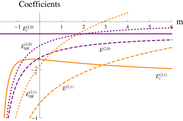
Figure 2: Coefficients of the exact (dashed), HF (dotted) and correlation (solid) energies with respect to $m$, for $v(r)=1$ (Eqs. (75), (76) and (77)).

Expanding (96) and (99) in terms of $Z$ and $D$ yields

$$E^{(2,0)}(V) =-\frac{1}{8}-\frac{1}{2(m+2)},$$ (100)

$$E_{\rm HF}^{(2,0)}(V) =-\frac{1}{2(m+2)},$$ (101)

thus showing that both $E^{(2,0)}$ and $E_{\rm HF}^{(2,0)}$ depend on the leading power $m$ of the external potential but not on $v(r)$.

Subtracting these energies yields

$$E_{\rm c}^{(2,0)}(V)=-\frac{1}{8},$$ (102)

and this completes the proof that, in the high-density limit, the leading coefficient $E_{\rm c}^{(2,0)}$ of the large-$D$ expansion of the correlation energy is universal, i.e. it does not depend on the external potential $V(r)$.

The result (102) is related to the cusp condition Kato57 ; Morgan93 ; Pan03

$$\left.\frac{\partial\Psi_{D}}{\partial r_{12}}\right|_{r_{12}=0}=\frac{1}{D-1}\Psi_{D}(r_{12}=0),$$ (103)

which arises from the cancellation of the Coulomb operator singularity by the $D$-dependent angular part of the kinetic operator Helgaker .

The $E^{(2,1)}$ and $E_{\rm HF}^{(2,1)}$ coefficients can be found by considering the Langmuir vibrations of the electrons around their equilibrium positions Herschbach86 ; Goodson87 . The general expressions depend on $v_{0}$ and $v_{1}$, but are not reported here. However, for $v(r)=1$, which includes many of the most common external potentials, we find

$$E_{\rm c}^{(2,1)}(V)=-\frac{85}{128}-\frac{9/32}{(m+2)^{3/2}}\\ +\frac{1/2}{(m+2)^{1/2}}+\frac{1/16}{(m+2)^{1/2}+2},$$ (104)

showing that $E_{\rm c}^{(2,1)}$, unlike $E_{\rm c}^{(2,0)}$, is potential-dependent. Numerical values of $E_{\rm c}^{(2,1)}$ are reported in Table 4 for various systems, and the components of the correlation energy are shown graphically in Fig. 2.

IV Conclusion

In this paper, we have reviewed our recent progress in the determination of the high-density correlation energy for four two-electron systems: the helium atom (He), the Hooke’s law atom (Ho), two electrons confined on the surface of a sphere (Sp), and two electrons trapped in a ball (Ba). In the large-$Z$ limit for $D=3$, we have found

$$E_{\rm c}({\rm He})\approx E_{\rm c}({\rm Sp})\approx E_{\rm c}({\rm Ho})\approx E_{\rm c}({\rm Ba}).$$ (105)

These striking similarities can be rationalized by treating the dimensionality $D$ of space as a system parameter, and we have proved that, as $D$ grows, all such correlation energies exhibit the same universal behaviour

$$E_{\rm c}\sim-1/(8D^{2})$$ (106)

in a $D$-dimensional space. This is true irrespective of the nature of the external potential that confines the electrons.

- (1) A. Szabo, N. S. Ostlund, Modern Quantum Chemistry : Introduction to Advanced Structure Theory, Dover publications Inc., Mineola, New-York, 1989.
- (2) T. Helgaker, P. Jørgensen, J. Olsen, Molecular Electronic-Structure Theory, John Wiley & Sons, Ltd., 2000.
- (3) C. White, B. G. Johnson, P. M. W. Gill, M. Head-Gordon, Chem. Phys. Lett. 253 (1996) 268.
- (4) E. Schwegler, M. Challacombe, J. Chem. Phys. 105 (1996) 2726.
- (5) M. C. Strain, G. E. Scuseria, M. J. Frisch, Science 271 (1996) 51.
- (6) J. C. Burant, G. E. Scuseria, M. J. Frisch, J. Chem. Phys. 105 (1996) 8969.
- (7) C. Ochsenfeld, C. A. White, M. Head-Gordon, J. Chem. Phys. 109 (1998) 1663.
- (8) K. Kitaura, E. Ikeo, T. Asada, T. Nakano, M. Uebayasi, Chem. Phys. Lett. 313 (1999) 701.
- (9) Y. Komeiji, T. Nakano, K. Fukuzawa, Y. Ueno, Y. Inadomi, T. Nemoto, M. Uebaysai, D. G. Fedorov, K. Kitaura, Chem. Phys. Lett. 372 (2003) 342.
- (10) D. G. Fedorov, K. Kitaura, Chem. Phys. Lett. 433 (2006) 182.
- (11) J. L. Whitten, J. Chem. Phys. 58 (1973) 4496.
- (12) O. Vahtras, J. Almlöf, M. W. Feyereisen, Chem. Phys. Lett. 213 (1993) 514.
- (13) B. I. Dunlap, W. D. Connolly, J. R. Sabin, Int. J. Quantum Chem. Symp. 11 (1977) 81.
- (14) A. P. Rendell, T. J. Lee, J. Chem. Phys. 101 (1994) 400.
- (15) R. A. Kendall, H. A. Fruchtl, Theor. Chem. Acc. 97 (1997) 158.
- (16) F. Weigend, Phys. Chem. Chem. Phys. 4 (2002) 4285.
- (17) T. J. Martinez, E. A. Carter, Modern Electronic Structure Theory, Advanced Series in Physical Chemistry, World Scientific, Singapore, 1995, p. 1132.
- (18) R. A. Friesner, R. B. Murphy, M. D. Beachy, M. N. Ringnalda, W. T. Pollard, B. D. Dunietz, Y. Cao, J. Phys. Chem. A 103 (1999) 1913.
- (19) N. H. F. Beebe, J. Linderberg, Int. J. Quantum Chem. 12 (1977) 683.
- (20) I. Roeggen, E. Wisloff-Nilssen, Chem. Phys. Lett. 132 (1986) 154.
- (21) H. Koch, A. S. de Meras, T. B. Pedersen, J. Chem. Phys. 118 (2003) 9481.
- (22) F. Aquilante, T. B. Pedersen, R. Lindh, J. Chem. Phys. 126 (2007) 194106.
- (23) F. Aquilante, L. Gagliardi, T. B. Pedersen, R. Lindh, J. Chem. Phys. 130 (2009) 154107.
- (24) R. Jurgens-Lutovsky, J. Almlöf, Chem. Phys. Lett. 178 (1991) 451.
- (25) K. Wolinski, P. Pulay, J. Chem. Phys. 118 (2003) 9497.
- (26) W. Z. Liang, M. Head-Gordon, J. Phys. Chem. A 108 (2004) 3206.
- (27) R. P. Steele, R. A. DiStasio, Y. Shao, J. Kong, M. Head-Gordon, J. Chem. Phys. 125 (2006) 074108.
- (28) J. Deng, A. T. B. Gilbert, P. M. W. Gill, J. Chem. Phys. 130 (2009) 231101.
- (29) J. Deng, A. T. B. Gilbert, P. M. W. Gill, J. Chem. Phys. 133 (2010) 044116.
- (30) R. D. Adamson, J. P. Dombroski, P. M. W. Gill, Chem. Phys. Lett. 254 (1996) 329–336.
- (31) P. M. W. Gill, R. D. Adamson, Chem. Phys. Lett. 261 (1996) 105–110.
- (32) J. P. Dombroski, S. W. Taylor, P. M. W. Gill, J. Phys. Chem. 100 (1996) 6272.
- (33) S. A. Varganov, A. T. B. Gilbert, E. Deplazes, P. M. W. Gill, J. Chem. Phys. 128 (2008) 201104.
- (34) P. M. W. Gill, A. T. B. Gilbert, Chem. Phys. 356 (2009) 86–90.
- (35) T. Limpanuparb, P. M. W. Gill, Phys. Chem. Chem. Phys. 11 (2009) 9176–9181.
- (36) E. Wigner, Phys. Rev. 46 (1934) 1002–1011.
- (37) P.-O. Löwdin, Adv. Chem. Phys. 2 (1959) 207–322.
- (38) R. P. Feynman, Statistical mechanics, Addison-Wesley, 1989.
- (39) H. Nakashima, H. Nakatsuji, J. Chem. Phys. 127 (2007) 224104.
- (40) H. Nakashima, Y. Hijikata, H. Nakatsuji, J. Chem. Phys. 128 (2008) 154107.
- (41) H. Nakashima, H. Nakatsuji, J. Chem. Phys. 128 (2008) 154108.
- (42) Y. I. Kurokawa, H. Nakashima, H. Nakatsuji, Phys. Chem. Chem. Phys. 10 (2008) 4486.
- (43) C. Schwartz, Int. J. Mod. Phys. E 15 (2006) 877.
- (44) C. A. Coulson, A. H. Neilson, Proc. Phys. Soc. (London) 78 (1961) 831.
- (45) J. K. Pearson, P. M. W. Gill, J. Ugalde, R. J. Boyd, Mol. Phys. 07 (2009) 1089.
- (46) M. C. Per, S. P. Russo, I. K. Snook, J. Chem. Phys. 130 (2009) 134103.
- (47) P.-F. Loos, P. M. W. Gill, Phys. Rev. A 81 (2010) 052510.
- (48) P. M. W. Gill, D. L. Crittenden, D. P. O’Neill, N. A. Besley, Phys. Chem. Chem. Phys. 8 (2006) 15.
- (49) E. E. Dumont, D. L. Crittenden, P. M. W. Gill, Phys. Chem. Chem. Phys. 9 (2007) 5340.
- (50) D. L. Crittenden, P. M. W. Gill, J. Chem. Phys. 127 (2007) 014101.
- (51) D. L. Crittenden, E. E. Dumont, P. M. W. Gill, J. Chem. Phys. 127 (2007) 141103.
- (52) Y. A. Bernard, D. L. Crittenden, P. M. W. Gill, Phys. Chem. Chem. Phys. 10 (2008) 3447.
- (53) J. K. Pearson, D. L. Crittenden, P. M. W. Gill, J. Chem. Phys. 130 (2009) 164110.
- (54) J. W. Hollett, P. M. W. Gill, Phys. Chem. Chem. Phys. (2010) submitted.
- (55) H. A. Bethe, E. E. Salpeter, Quantum Mechanics of One- and Two-Electron Atoms, Dover Publications Inc., Mineola, New-York, 1977.
- (56) M. Gell-Mann, K. A. Brueckner, Phys. Rev. 106 (1957) 364.
- (57) G. F. Giuliani, G. Vignale, Quantum theory of electron liquid, Cambridge University Press, Cambridge, 2005.
- (58) R. G. Parr, W. Yang, Density Functional Theory for Atoms and Molecules, Oxford University Press, 1989.
- (59) P.-F. Loos, P. M. W. Gill, J. Chem. Phys. 131 (2009) 241101.
- (60) P.-F. Loos, P. M. W. Gill, Phys. Rev. Lett. (2010) in press arXiv:1005.0676v4.
- (61) E. A. Hylleraas, Z. Phys. 65 (1930) 209.
- (62) J. Linderberg, Phys. Rev. 121 (1961) 816.
- (63) E. A. Hylleraas, Adv. Quantum Chem. 1 (1964) 1.
- (64) F. W. J. Olver, D. W. Lozier, R. F. Boisvert, C. W. Clark (Eds.), NIST handbook of mathematical functions, Cambridge University Press, New York, 2010.
- (65) D. R. Herrick, F. H. Stillinger, Phys. Rev. A 11 (1975) 42.
- (66) J. D. Baker, D. E. Freund, R. N. Hill, J. D. Morgan III, Phys. Rev. A 41 (1990) 1247.
- (67) W. Kutzelnigg, J. D. Morgan III, J. Chem. Phys. 96 (1992) 4484.
- (68) D. R. Herrick, J. Math. Phys. 16 (1975) 281.
- (69) W. Byers Brown, J. O. Hirschfelder, Proc. Natl. Acad. Sci. USA 50 (1963) 399–406.
- (70) P.-F. Loos, P. M. W. Gill, Phys. Rev. A 79 (2009) 062517.
- (71) P.-F. Loos, P. M. W. Gill, Phys. Rev. Lett. 103 (2009) 123008.
- (72) P.-F. Loos, Phys. Rev. A 81 (2010) 032510.
- (73) P.-F. Loos, P. M. W. Gill, Mol. Phys. (2010) in press arXiv:1004.3641v2.
- (74) G. S. Ezra, R. S. Berry, Phys. Rev. A 25 (1982) 1513.
- (75) G. S. Ezra, R. S. Berry, Phys. Rev. A 28 (1983) 1989.
- (76) P. C. Ojha, R. S. Berry, Phys. Rev. A 36 (1987) 1575.
- (77) R. J. Hinde, R. S. Berry, Phys. Rev. A 42 (1990) 2259.
- (78) J. W. Warner, R. S. Berry, Nature 313 (1985) 160.
- (79) M. Seidl, Phys. Rev. A 75 (2007) 062506.
- (80) M. Seidl, J. P. Perdew, S. Kurth, Phys. Rev. Lett. 84 (2000) 5070.
- (81) A. G. Ushveridze, Quasi-Exactly Solvable Models in Quantum Mechanics, Institute of Physics Publishing, 1994.
- (82) N. R. Kestner, O. Sinanoglu, Phys. Rev. 128 (1962) 2687.
- (83) E. Santos, Anal. R. Soc. Esp. Fis. Quim. 64 (1968) 177.
- (84) S. Kais, D. R. Herschbach, R. D. Levine, J. Chem. Phys 91 (1989) 7791.
- (85) M. Taut, Phys. Rev. A 48 (1993) 3561.
- (86) J. Katriel, S. Roy, M. Springborg, J. Chem. Phys. 123 (2005) 104104.
- (87) P. M. W. Gill, D. P. O’Neill, J. Chem. Phys. 122 (2005) 094110.
- (88) R. J. White, W. Byers Brown, J. Chem. Phys. 53 (1970) 3869–3879.
- (89) J. Cioslowski, K. Penal, J. Chem. Phys. 113 (2000) 8434.
- (90) A. Alavi, J. Chem. Phys. 113 (2000) 7735.
- (91) D. C. Thompson, A. Alavi, Phys. Rev. B 66 (2002) 235118.
- (92) D. C. Thompson, A. Alavi, J. Chem. Phys. 122 (2005) 124107.
- (93) J. Jung, J. E. Alvarellos, J. Chem. Phys. 118 (2003) 10825.
- (94) J. Jung, P. Garcia-Gonzalez, J. E. Alvarellos, R. W. Godby, Phys. Rev. A 69 (2004) 052501.
- (95) D. C. Thompson, A. Alavi, Phys. Rev. B 69 (2004) 201302.
- (96) D. C. Thompson, A. Alavi, J. Phys.: Condens. Matter 16 (2004) 7979.
- (97) P.-F. Loos, P. M. W. Gill, J. Chem. Phys. 132 (2010) 234111.
- (98) L. G. Yaffe, Rev. Mod. Phys. 54 (1982) 407.
- (99) E. Witten, Physics Today 33 (1980) 38.
- (100) L. G. Yaffe, Physics Today 36 (1983) 50.
- (101) D. R. Herschbach, J. Chem. Phys. 84 (1986) 838.
- (102) D. Z. Goodson, D. R. Herschbach, J. Chem. Phys. 86 (1987) 4997.
- (103) D. J. Doren, D. R. Herschbach, Phys. Rev. A 34 (1986) 2654.
- (104) D. J. Doren, D. R. Herschbach, J. Chem. Phys. 87 (1987) 443.
- (105) D. Z. Goodson, M. López-Cabrera, D. R. Herschbach, J. D. Morgan III, J. Chem. Phys 97 (1992) 8481.
- (106) D. Z. Goodson, M. López-Cabrera, Low-D regime: the one-dimensional limit, Dimensional Scaling in Chemical Physics, Kluwer Academic Publishers, Dordrecht, 1993, p. 115.
- (107) J. G. Loeser, D. R. Herschbach, J. Chem. Phys. 86 (1987) 2114.
- (108) J. G. Loeser, D. R. Herschbach, J. Chem. Phys. 86 (1987) 3512.
- (109) J. G. Loeser, J. Chem. Phys. 86 (1987) 5635.
- (110) S. Kais, S. M. Sung, D. R. Herschbach, J. Chem. Phys 99 (1993) 5184.
- (111) L. D. Mlodinow, N. Papanicolaou, Ann. Phys. 131 (1981) 1.
- (112) T. Kato, Commun. Pure Appl. Math. 10 (1957) 151.
- (113) J. D. Morgan III, The dimensional dependence of rates of convergence of Rayleigh-Ritz variational calculations on atoms and molecules, Dimensional Scaling in Chemical Physics, Kluwer Academic Publishers, Dordrecht, 1993, p. 336.
- (114) X.-Y. Pan, V. Sahni, J. Chem. Phys. 119 (2003) 7083.