A Novel Association Policy for Web Browsing in a Multirate WLAN

Abstract

We obtain an association policy for STAs in an IEEE 802.11 WLAN by taking into account explicitly two aspects of practical importance: (a) TCP-controlled short file downloads interspersed with read times (motivated by web browsing), and (b) different STAs associated with an AP at possibly different rates (depending on distance from the AP).

Our approach is based on two steps. First, we consider an analytical model to obtain the aggregate AP throughput for long TCP-controlled file downloads when STAs are associated at $k$ different rates $r_{1}$, $r_{2}$, $\ldots$, $r_{k}$; this extends earlier work in the literature. Second, we present a 2-node closed queueing network model to approximate the expected average-sized file download time for a user who shares the AP with other users associated at a multiplicity of rates. These analytical results motivate the proposed association policy, called the Estimated Delay based Association (EDA) policy: Associate with the AP at which the expected file download time is the least.

Simulations indicate that for a web-browsing type traffic scenario, EDA outperforms other policies that have been proposed earlier; the extent of improvement ranges from 12.8% to 46.4% for a 9-AP network. To the best of our knowledge, this is the first work that proposes an association policy tailored specifically for web browsing. Apart from this, our analytical results could be of independent interest.

I Introduction

IEEE 802.11a/b/g/n based Wireless LAN are used for providing Internet access in many places. In most deployed network a single station (STA) can see multiple access points (APs) as shown in Figure 1. In this situation, STAs associate with a particular AP. Usually, association of STA with AP is based on SNR. This simple scheme ignores the fact that some APs are loaded heavily while some are underutilized. Hence, load imbalance and lower throughput are some common problems. Prior and contemporary works address these problems by assuming a saturated traffic model. They assume that at any point of time, every STA is hungry to send packets across and is always contending for the channel. However, according to the statistics given in [1], 46% of Internet traffic is attributed to web browsing, which is more intermittent than saturated. The reason that it is intermittent rather than saturated is that TCP involved; we will discuss this in more detail shortly.

Figure 1: Associated STAs are downloading the files from a server through APs and a new STA arrived to region, where it can potentially get associated with any one of the APs

While TCP-controlled file downloads in WLANs have been studied in [2], it was assumed that all STAs are associated with the AP as a single rate. In reality, multiple rates are possible; for example, 802.11g offers 8 rates of association. The study of TCP-controlled file transfers with multiple rates of association has received little attention in the literature; a first step was taken in [3].

Even though the literature on association policies is extensive, the vast majority of the works considers the saturated traffic model. Given the prevalence of TCP-controlled traffic, which does not correspond to the saturated model, and the fact that multiple rates of STA-AP association are possible, one begins to wonder if policies based on a different approach can perform better. Clearly, if this were possible, a very substantial number of WLAN users would stand to benefit.

This question motivates the work reported in this paper. We obtain an association policy for STAs in an IEEE 802.11 WLAN by taking into account explicitly two aspects of practical importance: (a) TCP-controlled short file downloads interspersed with read times (motivated by web browsing), and (b) different STAs associated with an AP at possibly different rates (depending on distance from the AP).

Figure 2: Two scenarios, the left side one with the saturated traffic and the right side one with unsaturated traffic. The queues of the AP and STAs are shown next to them. In the saturated traffic case both the AP and the STAs have packets in its queue all the time. In the unsaturated traffic scenario which we are addressing, the AP only have packets to transmits all the time and the MAC queues at STAs are empty most of the time.

To see why unsaturated traffic makes a difference, we consider Figure 2. The left part shows a saturated traffic scenario, where all WLAN entities have packets to transmit; therefore, $(N+1)$ entities contend for the channel. The right part shows the situation with TCP in the picture. Essentially, for many TCP connections, the entire window of packets sits at the AP, leaving the corresponding STAs with nothing to send. This means that the number of contending WLAN entities is much smaller [2]. This suggest why approaches relying on saturated traffic may be inadequate.

We approach the problem in two steps. First, we consider an analytical model to obtain the aggregate AP throughput for long TCP-controlled file downloads when STAs are associated at $k$ different rates $r_{1}$, $r_{2}$, $\ldots$, $r_{k}$; this extends earlier work in the literature. Second, we present a 2-node closed queueing network model to approximate the expected average-sized file download time for a user who shares the AP with other users associated at a multiplicity of rates. These analytical results motivate the proposed association policy, called the Estimated Delay Based (EDA) policy: Associate with the AP at which the expected file download time is the least. To summarize, our approach can be depicted as shown in Figure 3.

Our contributions are as follows:
(i) We derive a closed form expression for the aggregate throughput of an AP with which STAs are associated at multiple data rates. Simulations indicate a very good match with analytical results.
(ii) We obtain a closed form expression for the mean delay experienced by an STA in downloading an average sized file. Again, simulation results match the analysis very well.
(iii) Utilizing these results, we present an on-line, distributed, client-driven association policy (EDA) which gives substantially increased throughput for every STA with balanced load among the APs; throughputs are observed to improve by 12.8% to 46.4%.

Figure 3: Approach of the modelling and application of the model

Outline of the paper: In Section II we provide a brief overview of related work. In Section III we state the assumptions, describe our models and introduce notations. In Section IV, we analyze a model for aggregate throughput of an AP with multi-rate association. Section V covers the analysis of average download time in a multirate scenario. In Section VI, we present a new distributed association policy based on the average file download delay. In Section VII, we provide simulation results that compare EDA policy with the SNR-based and aggregate throughput maximizing schemes. In Section VIII we discuss the results and identify future research directions. Finally, in Section IX, we conclude the paper.

II Related Work

From the extensive literature on association in WLANs, several themes can be discerned. In the first group, a newcomer STA assesses each AP (that it can hear) by finding out the per-STA throughput received by STAs associated with it currently [20], [22] and [23]. In these papers, the authors derive expressions for aggregate AP throughput (with UDP traffic), taking into account the number of STAs associated, as well as the probability of packet loss due to collisions. From this, the per-STA throughput can be calculated, and the newcomer associates with the AP for which the per-STA throughput is the highest.

In the second group, we have association policies that start from the throughputs that individual STAs are getting at present [10], [12], [14], [15] and [18]. For each STA associated with an AP, the ratio of throughput to the physical rate of association is obtained, and this fraction is added over all the STAs. This leads to a figure of merit for each AP, and the newcomer chooses the AP with the highest figure of merit.

For a brief overview of the other categories, let us assume that a newcomer STA can hear 3 APs denoted as $a$, $b$ and $c$, with $n_{a}$, $n_{b}$ and $n_{c}$ STAs (respectively) associated with them. Suppose the new AP associates with AP $a$. Then, one can imagine an $(n_{a}+n_{b}+n_{c}+1)$ -element vector $\overline{v_{a}}$, listing the throughputs of all STAs in the system. Similarly, there would be vectors corresponding to choosing AP $b$ $\overline{v_{b}}$ and AP $c$ $\overline{v_{c}}$.

In the third group, the selection of the AP is made by considering Jain’s fairness index $JF(\overline{v_{a}})$, $JF(\overline{v_{b}})$ and $JF(\overline{v_{c}})$, corresponding to $v_{a}$, $v_{b}$ and $v_{c}$ respectively. The AP selected is the one for which the Jain Fairness Index is the highest [24]. In the fourth group, $\overline{v_{x}}$ is mapped to an expression for AP load $(x=a,b,c)$, and the AP which is least loaded is selected. A variation considers a map from the vector of throughputs $(\overline{v_{x}})$ and the vector of rates of association to the load [5] . Finally, some association policies base their choice on maximizing the minimum element of $\overline{v_{a}}$, $\overline{v_{b}}$ and $\overline{v_{c}}$ (“max-min fairness”), or maximizing the sum of the logarithms of the elements of $\overline{v_{x}}$, $x=(a,b,c)$, [7], [9], [11], [13], and [19].

A common assumption in all these policies is that of saturated traffic, viz., all WLAN entities have packets to send always.

IEEE 802.11$k$ [29] define several metrics for radio resource management, including channel load report, BSS average access delay and BSS load. Any STA can request for channel load report. Other load metrics are broadcast by AP in beacon frames. These metrics can be utilized in arriving at association decisions.

The proposed EDA policy leverages the capabilities provided by 802.11$k$.

III Problem Statement and Models

Our goal is to look for an association policy that takes into account the specifics of TCP-controlled file transfers. To move towards this goal, our approach is to model two aspects: The aggregate AP throughput achievable in a multirate scenario and the expected time to download a file. Models for these two aspects are developed in Section III-B and III-C respectively. In Section III-A, we discuss the general assumptions that we have made.

Figure 4: Fixed number of STAs downloading files from a server which are connected through an AP. No new arrival or departure of the STA

III-A General assumptions

We consider a single cell 802.11 a/b/g/n of $M$ (large) STAs associated with a single AP as shown in Figure 4. All nodes are contending for the channel using the DCF mechanism. STAs are associated with the AP at $k$ different physical rates. We assume that there are no link error and packets in the medium are lost due to collisions only. The AP is connected to a file server by a wire as shown in Figure 4. In this paper, we assume that round trip time (RTT) is very small.

III-B Model for aggregate AP throughput

Each STA has a single TCP connection to download a large file from a local file server. In other words, the traffic model is homogeneous across STAs and no other traffic is present. The AP delivers TCP packets towards STAs and an STA returns TCP-ACK packets. There are several simultaneous TCP connections; every STA and the AP is contending for the channel. Further, as no preference is given to the AP, the AP is modelled as being backlogged permanently [2]. We assume that the AP uses the RTS-CTS mechanism while sending packets to the STAs and an STA uses basic access to send TCP-ACK packets. As soon as an STA receives a data packet, it generates a TCP-ACK packet without any delay and this is placed in the MAC queue. Also, we assume that all the nodes have sufficiently large buffer space, so that packets are not lost due to buffer overflow. Moreover, recovery form collision occurs before TCP time outs and TCP start-up transients are ignored.

III-C Model for estimating file download time

We consider a given AP and a fixed number of STAs associated with it; in other words, no new STA arrives and no associated STA leaves the system. Aggregate throughput of the AP is shared equally among all $M$ STAs. Hence the AP is modelled as a processor sharing queue. We assume that a file downloaded by an STA can belong to one of $L$ different classes, A file of class $l$, $1\leq L$, is distributed exponentially, with mean size $1/\mu_{l}$. After downloading a file, an STA goes into the “reading” state. For a class $l$ file, the reading time is distributed exponentially also, with the mean being $1/\lambda_{l}$. The reading state is modelled by a ./M/$\infty$ queue. Further, upon completion of reading, an STA downloads a fresh file of random size having mean $1/\mu_{l}$ with probability $q_{l}$, $\sum_{l=1}^{L}q_{l}=1$. Together, the AP queue and the “reading” queue constitute a closed queueing network.

Figure 5: A closed queue network model in which constant number of STAs alternating between Processor Sharing server (AP) and $M/M/\infty$ server

IV Aggregate AP Throughput Model

In this section, we are interested in obtaining a method to compute the aggregate throughput achieved by the AP. We assume that each STA is downloading an infinitely long file from a server attached to the AP via a wired network (for example, an Ethernet cable). A TCP packet transmitted to any STA is considered in obtaining the throughput expression; hence the resulting expression yields the aggregate throughput across all TCP connections. The result obtained here will be used as a part of the model presented in the next section.

Packets for every STA have to go through the AP and every STA replies with a TCP-ACK. Hence, all STAs along with the AP are contending for the channel. The AP does not have any preference over STAs, and it is modelled as being backlogged permanently. In this condition, we can model the performance of the AP as in [4].

The basic approach is to consider consecutive successful transmissions by the AP or one of the STAs. At these epochs, we consider the number of STAs at rate $r_{i}$, $1\leq i\leq k$, with TCP-ACK packets in them. This $k$-element non negative vector, embedded at consecutive successful transmission epochs, can be seen to be a Discrete Time Markov Chain (DTMC), and this DTMC is part of a Markov Renewal sequence defined at the consecutive success epochs. To obtain the aggregate AP throughput, we appeal to the Renewal Reward Theorem [27], where a reward of 1 accrues at every successful transmission by the AP. Owing to lack of space, we provide only a sketch of the argument; more details can be found in [4].

Let $M_{i}$ be the number of STAs associated with the AP at rate $r_{i}$, where $i\in\{1,2,\dots k\}$. The analysis proceeds by assuming $M_{i},1\leq i\leq k,$ to be large.

Figure 6: Embedded Markov chain formed by an AP and STAs associated with the AP at $k$ different data rates

As in [4] we can get the aggregate TCP throughput of the AP as

$$\Phi_{AP-TCP}=\frac{\Sigma^{\infty}_{n_{1}=0}\Sigma^{\infty}_{n_{2}=0}...\Sigma^{\infty}_{n_{k}=0}\pi(n_{1}...n_{k})\frac{1}{n_{1}+...+n_{k}}}{\Sigma^{\infty}_{n_{1}=0}\Sigma^{\infty}_{n_{2}=0}...\Sigma^{\infty}_{n_{k}=0}\pi(n_{1}...n_{k})E_{n_{1},..n_{k}}X}$$ (1)

where $\pi(n_{1},n_{2},...,n_{k})$ is the equilibrium probability of the DTMC being in state $(n_{1},n_{2},...,n_{k})$ , $X$ is the sojourn time in a DTMC state and $E_{n_{1},n_{2},...,n_{k}}X$ is the expected sojourn time, given that the DTMC state is $(n_{1},n_{2},...,n_{k})$.

To verify the accuracy of the model, we performed experiments using the Qualnet 4.5 network simulator [30]. We considered 802.11b physical data rates as 1Mbps, 2Mbps, 5.5Mbps and 11Mbps, depending on the physical distance from the AP. In Table II, results are given for a few cases of this multirate scenario, i.e., with different number of stations.

Total no.	No. of STAs with rate				Aggregate Throughput
of STAs	11	5.5	2	1	Analysis	Simulation	Error %
10	2	3	2	3	2.54	2.52	0.7
	1	2	3	4	2.57	2.53	1.6
12	2	2	4	4	3.49	3.45	1.2
	4	4	2	2	2.06	2.01	2.5

TABLE I: Analysis and Simulation Results [Mbps] for multirate AP in IEEE 802.11b

Detailed analysis is provided in [4]. From Table I, we see that the analytical approach yields results that are very close to those obtained from simulations. In the next section, the method to calculate aggregate AP throughput will be used to parameterize the model that will be presented.

V Short File download delay model

In this section, our goal is to obtain a figure of merit for a particular AP; the figure of merit reflects the performance that can be expected if a newly arrived STA associates with this AP, given its current “association state” (that is, for each rate $r_{1},r_{2},...,r_{k}$, the number of STAs associated with the AP at present). The question we address in this section is: If the current association state of the AP remains unchanged for a long time, what is the performance that a newly arrived STA can expect upon associating with this AP?

To recall our model in Section III-C: Each user alternates between downloading a finite-sized file and reading it. The downloaded files belong to $L$ classes; all files are distributed exponentially, and each class corresponds to a distinct mean file size. When a user downloads, the file is of class $l$ with probability $q_{l}$; at each download, the file class is chosen independently. This behaviour applies to each user; in other words, use homogeneity is assumed.

We consider a 2-node closed queueing network with the number of customers equal of the total number of STAs associated with the AP (Figure 5). Node 1 represents the AP, and node 2 represents the “reading station”. Node 1 is a Processor Sharing service station, because the AP may be considered to be sharing its aggregate throughput among the STAs that are downloading actively. Node 2 is modelled as an infinite server service station; it captures the reading times spent in reading files that have been downloaded already. At a given instant, the number of customers at node 1 is equal to the number of STAs downloading files at that instant. The number of customers at node 2 is equal to the number of STAs that are reading at that instant. The service rate of the server at node 1 is set to the aggregate AP throughput obtained in Section III. The service rates of the servers at node 2 depend on the customer class.

We remark upon two key modelling assumptions that we make in this section. The first is that all wireless-specific aspects are encapsulated in the service rate of node 1. Thus, the details of the number of STAs associated at the rates $r_{1}$, $1\leq i\leq k$, influence the service rate of node 1; nothing else in the 2-node model is specific to a wireless context. The second modelling assumption is that even though the aggregate AP throughput was obtained (in Section IV) for a scenario where infinitely large files were being downloaded, the same expression is used in the current context, where finite-sized files are being downloaded. Both assumptions are made for tractability and simplicity. Not making these assumptions lead to much more complex models, and it is not clear that these can be analyzed; even if analytical treatment is possible, it is unclear whether the improvements in the results would justify the complexity.

Ultimately, the figure of merit that we wish to compute is the average time taken to download a file, given the current association state of the AP.

Let the service rate of the AP be $\tau$. Let us consider $m_{1}$ STAs to be at node 1. That is, $m_{1}$ among $M$ STAs are busy in downloading files. These STAs can download files with mean size $\frac{1}{\mu_{1}}$ or $\frac{1}{\mu_{2}}$ … $\frac{1}{\mu_{L}}$. Now $m_{2}$ out of $M$ STAs are in read state. The state of the network can be represented by $S=(x_{1},x_{2})$. Here, $x_{i}$ is a vector with elements $m_{i,l}$; where $m_{i,l}$ is the number of customer of class $l$ at node $i$, (index $i$ is for node number and $l$ for class), $i\in\{1,2\}$, $l\in\{1,2,\dots L\}$. Also $m_{i}=\sum_{l=1}^{L}m_{i,l}$.

At node 1, the STA chooses the class $l$ with probability $q_{l}$, irrespective of its previous class. But, at node 2, an STA stays in the same class $l$, which it had chosen at node 1. Let $v_{i_{1},l_{1},i_{2},l_{2}}$ be the probability that a class $l_{1}$ STA at node $i_{1}$ becomes a class $l_{2}$ STA at node $i_{2}$. Then we have: $\begin{array}[]{c l}\mbox{$v_{1,l,2,l}=1$ }&\mbox{ $l\in\{1,2,...,L\}$}\\ \mbox{$v_{1,l,2,j}=0$ }&\mbox{ $j\neq l$}\\ \mbox{$v_{2,l^{\prime},1,l}=q_{l}$}&\mbox{ $(l,l^{\prime})\in\{1,2,...L\}$ }\end{array}$ For every $i$, let $e_{i,l}$ be the fraction of transitions into class $l$ center $i$. Then we have:

$$e_{i,l}=\sum_{(i^{\prime},l^{\prime})}(e_{i^{\prime},l^{\prime}})v_{i^{\prime},l^{\prime},i,l}$$ (2)

After solving the above equations,

$$e_{1,l}=\frac{q_{l}}{q_{1}}e_{1,1}=e_{2,l}$$ (3)

$e_{i,l}$ is determined to within a multiplicative constant. $e_{i,l}$ can be interpreted as the relative arrival rate of class $l$ customers to service center $i$.

This is a 2-node BCMP network [28]. The processor sharing server in Figure 5 is a type 2 server, and the ./M/$\infty$ is a type 3 server in the terminology of [28]. The expression for the service rate of node 1 is given by $\Phi_{AP-TCP}$ in (1), and that of the node 2 server is $1/\lambda_{l}$ for class $l$ customers. By the BCMP theorem [28], the equilibrium probabilities are given by

$$P(S=x_{1},x_{2})=Cd(S)f_{1}(x_{1})f_{2}(x_{2})$$ (4)

where $C$ is the normalizing constant chosen to make the equilibrium state probabilities sum to 1. $d(S)$ is a function of the number of customers in the system, and $f_{i}$ is a function that depends on the type of service center $i$.

From [28], for the Processor Sharing Server, Node 1,

$$f_{1}(x_{1})=m_{1}!\Pi_{l=1}^{l=L}\frac{1}{m_{1,l}!}(\frac{e_{1,l}}{\tau})^{m_{1,l}}$$ (5)

and for the infinite server, Node 2,

$$f_{2}(x_{2})=\Pi_{l=1}^{l=L}\frac{1}{m_{2,l}!}(\frac{e_{2,l}}{\lambda_{l}})$$ (6)

For a closed network, $d(S)=1$.

The average number of active STAs, $n_{avgDS}$ and average number of reading stations $n_{avgRS}$ can be obtained by finding the marginal distributions from (4).

$$n_{avgDS}=\sum_{l\in\{1,2,...L\}}m_{1,l}P(m_{1,l})$$ (7)

From Figure 5 it is clear that

$$n_{avgDS}+n_{avgRS}=M\\$$

Let the throughput in the closed network of Figure 5 be $t_{H}$. Then, applying Little’s Theorem to node 2, we have

$$n_{avgRS}=t_{H}\times\sum_{l=1}^{L}q_{l}\frac{1}{\lambda_{l}}$$ (8)

Having obtained $t_{H}$ and $n_{avgDS}$ as above, we can calculate the average download delay d seen by STAs:

$$\textit{d}=\frac{n_{avgDS}}{t_{H}}$$ (9)

In Figure 7, we compare the results from analysis and simulation for a single cutomer class. The match is quite good.

Figure 7: Average delay seen by STAs for downloading exponentially distributed files with mean 200KB with read time of mean 90 seconds

Number of STAs with rate [Mbps]				Delay [s]
11	5.5	2	1	Analytical	Simulation	Error(%)
1	2	3	4	1.954	1.938	0.82
1	3	2	4	1.977	1.946	1.59
3	2	3	4	2.237	2.209	1.27
2	4	4	3	2.352	2.314	1.64
3	2	4	4	2.423	2.411	0.91

TABLE II: Comparison of analysis and simulation results for “delay model”.

Further, to verify the accuracy of the model, we considered a scenario with fixed number of STAs at different rates. Two different average file sizes with mean as 50KB ($1/\mu_{1}$) and 250KB ($1/\mu_{1}$) represent two different classes in our model. Any STA selects an exponentially distributed file of mean size 50KB with probability 0.6 ($q$) and selects the other type with probability 0.4 ($1-q$). After downloading the file of mean size $1/\mu_{1}$, an STA goes to read mode with an exponentially distributed duration of mean 25 seconds ($1/\lambda_{1}$). If the STA downloads random file with the other mean (i.e., $1/\mu_{2}$), it goes to read mode with random time of mean 100 seconds ($1/\lambda_{2}$). Finally, after completion of read time, STA forgets what it has chosen as mean size and selects a fresh file from the two classes with probabilities $q$ and $1-q$. The results are presented in Table II. The analytical values match the simulation results very well.

VI A new association policy

The basic idea of our association policy is simple: For each AP that the newly arrived STA hears from, a figure of merit (mean download delay) is computed as in the last section. Then, the decision is to associate with the AP with the best figure of merit.

To calculate the mean download delay, any STA needs to know only the number of STAs associated with the AP and their physical data rates. This “association state” can be obtained using IEEE 802.11$k$. If the mean file sizes are known to the STA, then it can calculate the expected delay d itself. We assume that the number of file classes $L$ and corresponding mean file sizes $1/\mu_{l}$, $1\leq l\leq L$, are available from offline measurements, from a repository like [32].

VI-A Algorithm

The following algorithm runs in every STA as soon as it arrives in the network

1:  Set Channel index, $c=0$

2:  Set AP index, $j=0$

3:  if  Scan Mode = Active then

4:     Send Probe Request frame

5:     Receive the Probe Response frame

6:  else

7:     Wait for Beacon frame

8:  end if

9:  Measure the signal strength and find out possible data rate

10:  Extract the $M_{i}$ and $r_{i}$ from received frame

11:  Calculated the expected delay $d_{j}$ for APs $j$ given by Equation 9

12:  Increment the AP index $j=j+1$

13:  Goto step number 5 for information from next AP on the same channel.

14:  Increment the Channel index $c=c+1$ and Goto step number 3 to scan the next channel

15:  Find out minimum of $d_{j}$ for all $j$ and across all the channels

16:  Send Association request to that AP.

VII Performance Evaluation

We present simulation results that evaluate the AP selection approach based on the average delay (EDA) discussed in the previous section. In particular, we compare the EDA AP selection scheme with the RSSI based selection scheme and other similar selection schemes.

VII-A Simulation setup

We have simulated association policies in the Qualnet 4.5 simulator. We enhanced the 802.11 MAC implementation in Qualnet 4.5. Small changes, like appending of extra information in beacon frames and probe frames, have been implemented in the AP module of the simulator. The AP keeps track of the number of STAs associated with it and the rates of association of those STAs. When transmitting beacon frames, it adds this extra information to the existing frame and broadcasts it. To handle the association policy in active scanning, the AP sends the same information in the probe response frame. We have implemented the algorithms explained in previous sections and corresponding changes required for the association schemes in the STA module.

VII-B Scenarios

We have used three scenarios to understand the performance of the proposed association scheme. In the first scenario shown in Figure 8, we placed 2 APs at a distance of 480 meters. So, an STA very near to one AP can hear the second AP’s signal with SNR corresponding to the lowest possible rate. STAs arrive according to a Poisson distribution with parameter $\nu$ to the region shown in Figure 8 which is served by 2 APs. STAs which arrive to the shaded region choose between APs; other STAs have no choice. Hence we considered spatial arrival of STAs to be non homogeneous. This is modelled using the parameter $P_{centre}$, which is the probability that an STA arrives within the shaded region shown in Figure 8. This is a parameter that can be varied and system performance can be studied. After arriving, every STA downloads a file; after completion of download, it goes to the read state and then again downloads next file. There are two classes of files ($L$=2). The file sizes are distributed exponentially with means 50KB and 750KB. Read times are distributed exponentially with means of 40 seconds and 120 seconds. After downloading a random number of files with mean 100, the STA departs from the BSS. We ran a large number of independent simulations with different seeds to obtain confidence intervals.

Figure 8: $P_{centre}$ is the fraction of STA arrivals to the shaded region for the 2 APs scenario. Distances for only two data rates are shown. The outer one is the maximum distance for lowest data rate. The inner circle is the maximum distance for the highest data rate

To verify and evaluate the scheme further, in the next simulation 4 APs are placed as shown in Figure 9. Here again the shaded region is the $P_{centre}$ fraction of complete area. This parameter is varied from 0.1 to 0.9 to study the system performance.

Figure 9: Scenario with 4 APs and ranges shown with dotted circles are highest and lowest physical transmission rate. Shaded region shows $P_{centre}$

And finally we took a scenario with 9 APs as shown in Figure 10. Placement of APs are done by considering radio range of the APs and STAs. Here in this case, to study the performance of system, the load of centre AP is varied by parameter $p_{center}$ as the probability of STAs which arrives to the shaded region. Distance between the access points are chosen such that any STA in shaded region will have option to choose between at least 2 APs. There is always a chance for neighbour APs to share the load of centre AP.

Figure 10: Scenario which shows the placements of 9 APs. Shaded region is the $P_{centre}$, fraction of overall arrival of STAs to complete region

VII-C Other Association Policies

This section focuses on how the proposed EDA policy performs in comparison with the SNR based scheme and other distributed association schemes.

A distributed association policy based on Available Admission Capacity (AAC) is presented in [16]. AAC is the fraction of time of an AP that a new STA can acquire. A new association metric based on this EVA (Estimated aVailable bAndwidth) is proposed. From this metric, an STA can predict the maximum achievable rate that it can get. This new metric considers multirate, greedy users. [6] and [8] propose association polices similar to this AAC based one.

To calculate AAC, traffic offered is calculated and the ratio of this with maximum possible traffic is found. The Ratio is used to determine the best AP. Similarly, to find EVA the expected back off interval is obtained. Then channel busy time and contention overhead are calculated. This information is used to select the AP.

We have chosen another client driven association policy for comparison. The number of associated STAs and the effect of loss of a packet is considered in [20] and [22], while proposing an association scheme. The load of the AP is defined by using these two parameters as, $(1-P_{error})/n$, where $P_{error}=c_{1}(RSSIc_{2}+c_{3})^{c_{4}}$ where $c_{1}$, $c_{2}$, $c_{3}$ and $c_{4}$ are constants, and $n$ is the number of STAs. The APs pass these information to STAs in beacon frames.

VII-D Comparison

We have implemented the above algorithm in the Qualnet 4.5 simulator. We used similar scenarios for comparison. Table III shows the comparison of other selected policies with our policy. Let $t_{u}$ be the time download time for a file of size $m_{u}$ and $L$ be the number of file transfers. Then $Th_{ij}=\frac{1}{L}\sum_{u=1}^{L}\frac{m_{u}}{t_{u}}$ is throughput of STA $i$ which is associated with AP $j$. The average throughput of all the APs is calculated by taking the sum of the throughput for each STA, which is given by:

$$Th_{avg}=\frac{1}{a}\sum_{j}\sum_{i}Th_{ij}$$ (10)

Where $a$ is the total number of APs in the network.

Scenario	EDA	Load Balancing	EVA	SNR based
2 AP	2.95$\pm$0.01	2.68$\pm$ 0.01	2.78$\pm$0.01	2.45$\pm$0.01
improvement		10%	6 %	18.3 %
4 AP	3.80$\pm$0.01	3.09$\pm$ 0.01	3.45$\pm$0.01	2.84$\pm$0.01
improvement		22.7%	10.1%	33.4%
9 AP	4.12$\pm$0.01	3.20$\pm$ 0.01	3.65$\pm$0.01	2.81$\pm$0.01
improvement		28.7%	12.8%	46.4%

TABLE III: Comparison of EDA with other policies

Throughput [MBps] with 95% confidence intervals obtained by simulation for 3 different scenarios shown in Figures 8, 9 and 10. $P_{centre}$ = 0.9, average file sizes of 50KB and 750KB with reading times as 40s and 120s respectively. Probability of selecting smaller file is 0.6. Arrival rate of STA is 0.5 per second.

The graph shown in Figure 11 is the average of 50 runs of the same experiment with the same parameters with different seeds. The arrival rate is chosen as 0.5 per second. The 95 % confidence interval is also shown in the graphs for the aggregate throughput. Similarly for the graph in Figure 12, the arrival rate STAs is 1 per second.

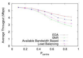
Figure 11: Throughput vs. $P_{centre}$ with arrival rate of STAs as 0.5 per second in the scenario of Figure 10 with 9 APs

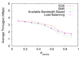
Figure 12: Throughput vs. $P_{centre}$ with arrival rate of STAs as 1 per second for scenario shown in Figure 10

It can be seen that EDA performs distinctly better than the other policies. From Figure 11, we see that the extent of improvement increases as the arrival process becomes more skewed spatially (higher values of $P_{centre}$ ). The relative improvement is not as appreciable in Figure [fig:Confidence_1ps], all APs are subjected to higher load, and different policies cease to make a significant difference.

Next we compare the four AP selection methods in terms of fairness. Jain’s fairness index [26] is used for the comparison. Jain’s Fairness Index is given by

$$\frac{(\sum_{i=1}^{M}T_{i})^{2}}{M\times\sum_{i=1}^{M}T_{i}^{2}}$$ (11)

where $M$ is the number of STAs and $T_{i}$ is the throughput of the $i^{th}$ STA. The fairness index lies in the range 1 to $1/M$. When one STA obtains all the capacity, the fairness index equals $1/M$. If the fairness index is 1, then all the STAs achieve equal throughputs. In Figure 13 we compare the fairness performance of the EDA policy with that of the others. It can be seen that the EDA and Available Bandwidth based policies achieve comparable degrees of fairness, which are distinctly better than those achieved by the others.

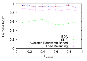
Figure 13: Fairness vs. $P_{centre}$ shows how the fairness index varies with increasing the load of centre AP in Figure 10

VIII Extensions

We presented an association policy by considering TCP-controlled file downloads. This traffic constitutes a very substantial part of network traffic, as mentioned in [1]. Now let us consider simultaneous TCP uploads. In DCF, A node’s attempt behaviour is independent of packet length. If we interchange downlink data packets sent by APs with TCP-ACK packets and uplink ACK packets sent by STAs with TCP data packets, the same analysis holds good for TCP-controlled file uploads. The next case arises when some STAs are uploading and some STAs are downloading files. Here also our basic Markov model of the number of STAs with packets to send remains the same, if all the TCP windows are equal. Even different window sizes can be taken care of by finding the probability that the packet at the head of the queue at the AP is for a particular STA.

Uncontrolled UDP transfers bring changes in the model and results. Apart from the above roaming is not addressed explicitly; it can be considered as a departure from one AP and an arrival to another AP. We considered a noise free environment. Introducing link errors by considering noisy environments may change the actual throughput compared to the one which we estimate before association. In our simulation and numerical evaluation, we used the 802.11b standard. However our mathematical expressions are independent of this standard; hence the association policy can support $k$ different data rates. Thus, we can apply the same scheme and analysis for 802.11g/n standards. We assumed small RTTs, clearly, this needs to be generalized, and we are working on this at present. Further, we considered exponentially distributed files with different mean sizes for different classes. As the BCMP network model supports file size distributions that are nonexponential also, our approach can accommodate these; however, the details are to be worked out.

IX Conclusion

We developed an STA-AP association policy geared towards TCP-controlled file downloads. Our approach was based on extending a model for studying TCP-controlled infinitely long file transfers to the multirate WLAN context, and incorporating the output from this in a 2-node closed-queueing network model for estimating finite file download times. The resulting policy showed considerable improvement over other policies, ranging from 12.8% better throughput compared to EVA, up to 46.4% better throughput compared to simple RSSI-based association for a 9-AP network.

The association policy developed here is but an application of the models analyzed in earlier sections. The models and the analytical approach may find use in addressing other performance evaluation questions. For example, they could be used to address some “what-if” questions like: What would be the performance benefit that can be expected by a network upgrade that introduces a few new APs to of load the traffic from already-deployed congested APs?

References

- [1] http://www.businesswire.com/news/google/20070618005912/en/Ellac oya-Data-Shows-Web-Traffic-Overtakes-Peer-to-Peer
- [2] G. Kuriakose, S. Harsha, A. Kumar, and V. Sharma, “Analytical models for capacity estimation of IEEE 802.11 WLANs using DCF for internet applications,” Wireless Networks, 2006.
- [3] Krusheel M and J. Kuri, “Performance Analysis of TCP Uploads in WLANs with Multiple Rates,” NCC 2009.
- [4] Pradeepa BK and J. Kuri, “Aggregate Download Throughput for TCP-controlled long file transfers in a WLAN with multiple STA-AP association rates”. Available: http://arxiv.org/pdf/1007.3229
- [5] G. S. Kasbekar, P. Nuggehalli, and J. Kuri, “Online client-AP association in WLANs,” Workshop on Resource Allocation in Wireless Networks (RAWNET), 2006
- [6] E. Garcia, J.L. Ferrer, E. L´opez, R. Vidal, and J. Paradells.“ Client-driven load balancing through association control in IEEE 802.11 WLANs.” European Transactions on Telecommunications, 20(5):494–507, August 2009.
- [7] Soung Chang Liew and Ying Jun Zhang, “Proportional Fairness in Multi- channel Multi-rate Wireless Networks”, IEEE Transactions on Wireless Communications, September 2008
- [8] Huazhi Gong and JongWon Kim, “Dynamic Load Balancing through Association Control of Mobile Users in WiFi Networks,” IEEE Transactions on Consumer Electronics, Vol. 54, No. 2, May 2008
- [9] Huazhi Gong, Kitae Nahm and JongWon Kim, “Distributed fair access point selection for multi-rate ieee 802.11 wlans,” 5th IEEE Consumer Communication and networking conference, 2008.
- [10] B Kauffmann, Fbaccelli, A Chaintreu, V Mhatre, K Papgiannaki and C Diot, “ Measurement Based Self Organizing of Interfering 802.11 Wireless Access Networks,” IEEE INFOCOM , 2007
- [11] V A Siris and D Evaggelatou, “Access Point Selection for Improving Throughput Fairness in Wireless LANs,” IEEE International Symposium on Integrated Network Management , 2007.
- [12] Murad Abusubaih, Sven Wiethoelter, James Gross and Adam Wolisz, “A new access point selection policy for multi-rate IEEE 802.11 WLANs,” International Journal of Parallel, Emergent and Distributed Systems, August 2008.
- [13] Li Li, Martin Pal and Yang Richard Yang, “ Proportional Fairness in Multi rate Wireless LANs,” IEEE INFOCOM 2008.
- [14] Ozgur Ekici and Abbas Yongacoglu, “A Novel Association Algorithm for Congestion Relief in IEEE 802.11 WLANs,” Proceedings of International Wireless Communications and Mobile Computing Conference, July 2006
- [15] Ozgur Ekici and A Yongacoglu, “Balanced Association algorithms for IEEE 802.11 extended service areas,” Wireless Communications and Mobile Computing , May 2008.
- [16] Heeyoung Lee, Seongkwan Kim, Okhwan Lee, Sunghyun Choi and Sung-Ju Lee, “ Available Bandwidth-Based Association in IEEE 802.11Wireless LANs,” ACM International Conference on Modeling, Analysis and Simulation of Wireless and Mobile Systems,MSWiM 2008.
- [17] Li-Hsing Yen, Tse-Tsung Yeh and Kuang-Hui Chi, “Load Balancing in IEEE 802.11 Networks,” IEEE Internet Computing , Feb 2009.
- [18] Yigal Bejerano, Seung-Jae Han and Li Li, “Fairness and Load Balancing in Wireless LANs Using Association Control,” IEEE Transactions on Networking June 2007, volume 15 No 3.
- [19] Yigal Bejerano and Seung Jae Han, “ Cell Breathing Techniques for Load Balancing in Wireless LANs,” IEEE Transactions on Mobile Computing, June 2009.
- [20] Y. Fukuda, A. Fujiwara, M. Tsuru and Y. Oie, “Analysis of access point selection strategy in wireless LAN,” IEEE Vehicular Technology Conference, 2005.
- [21] Y. Fukuda, M. Honjo, and Y. Oie. “ Development of Access Point Selection Architecture with Avoiding Interference for WLANs.” In The 17th IEEE International Symposium on Personal, Indoor and Mobile Radio Communications, PIMRC’06, September 2006.
- [22] Y. Fukuda and Y. Oie., “Decentralized Access Point Selection Architecture for Wireless LANs,” IECE Transactions on Communications , September 2007.
- [23] H. Al-Rizzo, M. Haidar, R. Akl, and Y. Chan. “Enhanced Channel Assignment and Load Distribution in IEEE 802.11 WLANs,” In IEEE International Conference on Signal Processing and Communications, ICSPC’07, November 2007.
- [24] Issam Jabri, Nicolas Krommenacker, Thierry Divoux, and Adel Soudani. “IEEE 802.11 Load Balancing: An Approach for QoS Enhancement.” International Journal of Wireless Information Networks, March 2008.
- [25] Quoc-Thinh Nguyen-Vuong, N. Agoulmine, and Y. Ghamri-Doudane. “A user-centric and context-aware solution to interface management and access network selection in heterogeneous wireless environments,” Computer Networks, December 2008.
- [26] R. Jain, D. Chiu, and W. Hawe. “A quantitative measure of fairness and discrimination for resource allocation in shared computer systems.” Technical Report TR-301, DEC Research, September 1984.
- [27] Anurag Kumar, “Discrete Event Stochastic Processes and Queueing Theory: Lecture Notes for an Engineering Curriculum,” http://www.ece.iisc.ernet.in/ anurag/
- [28] Baskett. F, Chandy. K. Mani, Muntz. R.R., Palacios, F.G. (1975). “Open, closed and mixed networks of queues with different classes of customers.” Journal of the ACM 22: 248–260. 1975.
- [29] IEEE 802.11 standard for Wireless Local Area Networks www.standards.ieee.org.
- [30] Qualnet Simulator, www.scalable-networks.com.
- [31] Ronal W. Wolff, “Stochastic Modeling and the Theory of Queues,” Prentice Hall 1989.
- [32] Traffic Generators for Internet Traffic, http://www.icir.org/models/trafficgenerators.html