Beyond Spherical Top Hat Collapse

Abstract

We study the evolution of inhomogeneous spherical perturbations in the universe in a way that generalizes the spherical top hat collapse in a straightforward manner. For that purpose we will derive a dynamical equation for the evolution of the density contrast in the context of a Lemaître-Tolman-Bondi metric and construct solutions with and without a cosmological constant for the evolution of a spherical perturbation with a given initial radial profile.

I Introduction

The formation of large scale structure in the universe is one of the most promising probes that will be used to determine fundamental cosmological parameters in future extra-galactic surveys, such as the imminent Dark Energy Survey (DES) Abbott:2005bi , the Large Synoptic Survey Telescope (LSST) Tyson:2003kb and the Euclid survey Euclid:2008eu .

The basic picture for large scale structure formation is that small perturbations generated by quantum fluctuations in the inflationary epoch grow in the dark matter to form gravitational potential wells where the baryons later fall into. The linear part of this process for dark matter is well understood and described by linear perturbation theory Bardeen:1980kt ; Kodama:1985bj . However, the nonlinear stages are not amenable to these perturbative methods even in the case when only dark matter is present. One then usually resorts to large numerical N-body simulations in order to obtain, e.g. the mass distribution of large dark matter haloes. Unfortunately, these simulations are very costly and it is desirable that a simple, approximate semi-analytical approach could be used to estimate the properties of dark matter haloes.

One such model is the so-called spherical collapse model Gunn:1972sv . In this extremely simple model, a spherically symmetric region of homogeneous overdensity, called “top-hat” density profile, evolves inside a homogeneous expanding Universe. Symmetry arguments show that one can regard the overdense region as a mini-universe of positive curvature. Hence the Raychaudhury and continuity equations can be used to evolve the density and radius of the spherical region Padmanabhan ; Fosalba:1997tn . When combined with the Press-Schechter theory Press:1973iz this framework provides a statistical basis for structure formation from which the number density of dark matter haloes can be estimated.

The spherical collapse model has been recently used to study structure formation in models with a simple Yukawa-type modification of gravity Martino:2008ae , in the so-called $f(R)$ models Schmidt:2008tn , in braneworld cosmologies Schmidt:2009yj , in models which allow for dark energy fluctuations Mota:2004pa ; Nunes:2004wn ; Nunes:2005fn ; Horellou:2005qc ; Manera:2005ct ; Schaefer:2007nf ; Abramo:2007iu ; Abramo:2008ip ; Basilakos:2009mz ; Pace:2010sn ; Wintergerst:2010ui and in the so-called chameleon models Brax:2010tj . The purpose of this work is to relax the assumption of a top-hat profile and study the nonlinear evolution of an inhomogeneous spherical perturbation in a fully relativistic framework.

II Evolution of an inhomogeneous spherical perturbation

In the case of an inhomogeneous perturbation one can not use a Friedmann-Robertson-Walker (FRW) metric which is valid only for a homogeneous matter distribution. The most general spherically symmetric metric is given by:

$$ds^{2}=e^{A(r,t)}dt^{2}-e^{B(r,t)}dr^{2}-R^{2}(r,t)d\Omega^{2}$$ (1)

where $t$ is the cosmic time, $r$ is the comoving radial coordinate and $d\Omega$ is the solid angle element. The metric is determined by three functions: $A(r,t)$, $B(r,t)$ and $R(r,t)$, where this last function is known as the areal radius since the area of a surface with a given time and comoving radial coordinates is given by $S=4\pi R(r,t)^{2}$. For a nice discussion on spherically symmetric inhomogeneous models see, e.g., chapter 18 in Plebanski:2006sd .

We assume a single perfect fluid with energy-momentum tensor given by

$$T_{\;\;b}^{a}=(\rho+p)u^{a}u_{b}-p\delta_{\;\;b}^{a}$$ (2)

where $\rho(r,t)$ and $p(r,t)$ are the energy density and pressure of the fluid and $u^{a}$ is its $4-$velocity, with $u^{a}u_{a}=1$. In a comoving reference frame $u=(e^{-A/2},\vec{0})$.

In this metric, Einstein equations with a cosmological constant, $G_{ab}-\Lambda g_{ab}=8\pi GT_{ab}$, can be written as:

$$e^{-A}\left(\frac{\dot{R}^{2}}{R^{2}}+\frac{\dot{B}\dot{R}}{R}\right)-e^{-B}\left(2\frac{R^{\prime\prime}}{R}+\frac{R^{\prime 2}}{R^{2}}-\frac{B^{\prime}R^{\prime}}{R}\right)+\frac{1}{R^{2}} = 8\pi G\rho+\Lambda$$ (3)

$$e^{-B}\left(2\frac{\dot{R}^{\prime}}{R}-\frac{\dot{B}R^{\prime}}{R}-\frac{A^{\prime}\dot{R}}{R}\right)=0$$ (4)

$$e^{-A}\left(2\frac{\ddot{R}}{R}+\frac{\dot{R}^{2}}{R^{2}}-\frac{\dot{A}\dot{R}}{R}\right)-e^{-B}\left(\frac{R^{\prime 2}}{R^{2}}+\frac{A^{\prime}R^{\prime}}{R}\right)+\frac{1}{R^{2}}=-8\pi Gp+\Lambda$$ (5)

$$\frac{e^{-A}}{4}\left(4\frac{\ddot{R}}{R}-2\frac{\dot{A}\dot{R}}{R}+2\frac{\dot{B}\dot{R}}{R}+2\ddot{B}+\dot{B}^{2}-\dot{A}\dot{B}\right)-$$

$$-\frac{e^{-B}}{4}\left(4\frac{R^{\prime\prime}}{R}+2\frac{A^{\prime}R^{\prime}}{R}-2\frac{B^{\prime}R^{\prime}}{R}+2A^{\prime\prime}+A^{\prime 2}-A^{\prime}B^{\prime}\right) = -8\pi Gp+\Lambda$$ (6)

where dots and primes refer to partial derivatives with respect to time and space, respectively.

Conservation of the energy-momentum tensor, $\nabla_{a}T_{\,\,b}^{a}=0$, in this spacetime results in the following equations:

$$\dot{B}+4\frac{\dot{R}}{R}+2\frac{\dot{\rho}}{\rho+p}=0$$ (7)

$$A^{\prime}+2\frac{p^{\prime}}{\rho+p}=0\,.$$ (8)

Equations (3) and (5), combined with Eq. (4), can be written as two conservation equations for the so-called active mass $m(r,t)$:

$$\frac{2m^{\prime}(r,t)}{R^{2}R^{\prime}} = 8\pi G\rho$$ (9)

$$\frac{2\dot{m}(r,t)}{R^{2}\dot{R}} = -8\pi Gp$$ (10)

with

$$2m(r,t)=e^{-A}R\dot{R}^{2}-e^{-B}RR^{\prime 2}+R-\frac{1}{3}\Lambda R^{3}\,.$$ (11)

We will focus on pressureless dark matter, in which case $p=0$ and

$$\dot{m}(r,t)=0\quad\Rightarrow\quad m=m(r).$$ (12)

In this case the metric takes the form of the Lemaître-Tolman-Bondi (LTB) metric Lemaitre:1933gd ; Tolman:1934za ; Bondi:1947av :

$$ds^{2}=dt^{2}-\frac{R^{\prime 2}}{1+f(r)}dr^{2}-R^{2}(r,t)d\Omega^{2}$$ (13)

where the curvature $f(r)$ is determined by $m(r)$ and $R$

$$f(r)=\dot{R}^{2}-\frac{2m(r)}{R}-\frac{1}{3}\Lambda R^{3}.$$ (14)

Models with large inhomogeneities described by a LTB metric, such as the so-called “Hubble bubble” model, have been used recently as an alternative explanation to the apparent acceleration of the universe (see, e.g Kolb:2005da ; Enqvist:2007vb ; GarciaBellido:2008nz ; Paranjape:2008ai ). Our goal here is to study the cosmological evolution of such an inhomogeneity.

The dynamical equations for the LTB model can be written as a generalization of the Friedmann equation

$$\frac{\dot{R}^{2}}{R^{2}}=\frac{2m(r)}{R^{3}}+\frac{f(r)}{R^{2}}+\frac{\Lambda}{3}$$ (15)

and a generalization of the “acceleration” equation

$$\frac{\ddot{R}}{R}=-\frac{m(r)}{R^{3}},$$ (16)

which is independent of the curvature, just like the FRW case. These equations reduce to the usual FRW equations if we set

$$R(r,t)=a(t)r$$ (17)

and

$$f(r)=-kr^{2},$$ (18)

where $k$ is the spatial curvature.

To describe the evolution of the inhomogeneous density perturbation we define the density contrast

$$\delta\left(r,t\right)\equiv\frac{\rho\left(r,t\right)-\overline{\rho}\left(t\right)}{\overline{\rho}\left(t\right)}$$ (19)

where $\rho(r,t)$ is the energy density inside the perturbation and $\overline{\rho}(t)$ is the energy density of the unperturbed expanding background.

The dynamical equation for $\delta(r,t)$ can be deduced from Eq. (7), which for a pressureless fluid becomes

$$\dot{\rho}+3h\rho=0$$ (20)

where $h\equiv\dot{b}/b$ and $b\equiv(R^{2}R^{\prime})^{1/2}$, together with the expanding background continuity equation:

$$\dot{\overline{\rho}}+3H\overline{\rho}=0\,$$ (21)

where $H=\dot{a}/a$. Taking the derivative of Eq. (19) with respect to time we obtain

$$\dot{\rho}=\dot{\overline{\rho}}\left(1+\delta\right)+\overline{\rho}\dot{\delta}\,,$$ (22)

which can be rewritten as

$$\dot{\delta}=3\left(H-h\right)\left(1+\delta\right)$$ (23)

where we have used Eqs. (20) and (21).

Deriving Eq. (23) with respect to time we obtain

$$\ddot{\delta}=3\left(\dot{H}-\dot{h}\right)\left(1+\delta\right)+3\left(H-h\right)\dot{\delta}\,.$$ (24)

If we now combine Eqs. (3)-(6) with the equations

$$\dot{H}=-\frac{3}{2}H^{2}+\frac{\Lambda}{2}$$ (25)

and

$$\dot{h}=4\pi G\rho+\frac{2}{3R}\left(\frac{f}{R}+\frac{f^{\prime}}{R^{\prime}}\right)+\Lambda-3h^{2}$$ (26)

Eq. (24) becomes the nonlinear differential equation for the evolution of the density perturbation:

$$\ddot{\delta}+2H\dot{\delta}-4\pi G\bar{\rho}\delta\left(1+\delta\right)-\frac{4}{3}\frac{\dot{\delta}^{2}}{1+\delta}=\frac{\Lambda}{2}\left(1+\delta\right)+\frac{2}{3}\left[\frac{\partial}{\partial t}\ln\frac{R}{R^{\prime}}\right]^{2}\left(1+\delta\right)\,.$$ (27)

Note that for a homogeneous density perturbation with a top-hat profile the areal radius is $R=ra$. In this case, the last term on the right hand side of Eq. (27) vanishes, reducing this equation to the well known evolution equation (see, e.g. Abramo:2007iu ) in the case of a single pressureless fluid.

Eq. (27) generalizes the evolution of $\delta$ for spherical perturbations with arbitrary initial radial profiles. Note, however, that for the simple case of pressureless dark matter, the solution of this equation can be obtained directly from Eqs. (20) and (9), which is what we will do in the following.

Consider initially a radial density profile expanding with the background

$$R_{i}=ra_{i}$$ (28)

which is characterized by a time-independent function $g(r)$

$$\rho_{i}\left(r\right)=\bar{\rho_{i}}\left\{1+\delta_{i}\left(r\right)\right\}=\bar{\rho_{i}}g\left(r\right)\,.$$ (29)

Since Eq. (9) in LTB is time-independent, we can set

$$4\pi GR_{i}^{2}R_{i}^{\prime}\rho_{i}\left(r\right)=4\pi GR^{2}R^{\prime}\rho\,.$$ (30)

Furthermore, since $\bar{\rho}_{0}=\bar{\rho}a^{3}$ and $\rho=\bar{\rho}\left\{1+\delta\right\}$ we obtain

$$\delta\left(r,t\right)=a\left(t\right)^{3}\frac{g\left(r\right)r^{2}}{R^{2}R^{\prime}}-1\,.$$ (31)

Defining a dimensionless areal radius

$$\widetilde{R}=\frac{R}{r},$$ (32)

Eq. (31) becomes

$$\delta\left(r,t\right)=a\left(t\right)^{3}\frac{g\left(r\right)}{\widetilde{R}^{2}\left[\widetilde{R}+r\widetilde{R}^{\prime}\right]}-1,$$ (33)

which is, of course, the formal solution to the nonlinear evolution equation Eq. (27).

Before we find the evolution of the density contrast we need to solve the dynamical equations of the background FRW metric for $a(t)$ and of the LTB metric for $\widetilde{R}(r,t)$.

III Solutions of the LTB model for a given initial density profile

We consider initially solutions of the LTB model applied to an inhomogeneous density perturbation with an initial density profile embedded in a Einstein-de Sitter and $\Lambda$CDM background.

III.1 Einstein-de Sitter background

Our first goal is to study the evolution of an initial spherically symmetric perturbation in a dark matter dominated universe with an Einstein- de Sitter (EdS) background in the context of General Relativity.

We assume that at an arbitrary initial time $t=t_{i}$, the whole universe follows the background expansion with $R(r,t_{i})=a(t_{i})r$, but has an initial small density perturbation specified by a profile $g(r)$:

$$\rho(r,t_{i})=\bar{\rho}(t_{i})g(r)$$ (34)

where $\bar{\rho}(t_{i})$ is the initial homogeneous background density.

Since $m(r)$ is time-independent it can be computed as:

$$m(r)=4\pi Ga_{i}^{3}\bar{\rho}_{i}\int_{0}^{r}dr^{\prime}r^{\prime 2}g(r^{\prime}).$$ (35)

Defining

$$h(r)=\frac{3}{r^{3}}\int_{0}^{r}dr^{\prime}r^{\prime 2}g(r^{\prime})$$ (36)

we can write

$$m(r)=\frac{4\pi G}{3}\bar{\rho}_{0}r^{3}h(r),$$ (37)

where the background density today is $\bar{\rho}_{0}=a_{i}^{3}\bar{\rho}_{i}$.

Using time in units of the Hubble age today

$$\tilde{t}=tH_{0}$$ (38)

and distance in units of the comoving radius

$$\tilde{R}=\frac{R}{r}$$ (39)

we will solve the acceleration equation

$$\frac{\partial^{2}\tilde{R}}{\partial\tilde{t}^{2}}=-\frac{1}{2}\Omega_{0}\tilde{R}^{-2}h(r)$$ (40)

for a given value of $r$ and initial conditions

$$\left(\frac{\partial\tilde{R}}{\partial\tilde{t}}\right)_{i}=\sqrt{a_{i}^{-1}\Omega_{0}+(1-\Omega_{0})}$$ (41)

and $\tilde{R}_{i}=a_{i}$.

Hence, given the initial conditions, the evolution of the inhomogeneous perturbation is completely determined by its initial profile. As an example of our method, we choose a Gaussian profile with width given by $r_{c}$ with a sharp cutoff at $r=r_{c}$ characterizing the comoving size of the perturbation:

$$g(r)=1+\delta_{i}e^{-r^{2}/r_{c}^{2}}\Theta(r_{c}-r)$$ (42)

where $\Theta(x)$ is the usual Heaviside function. We have started our evolution from $a_{i}=10^{-5}$ and chose $\delta_{i}=10^{-4.552}$, which results in the collapse today ($a=1$ when $\tilde{t}=0.667$) of the center of the perturbation. Exact solutions for the dynamical LTB equations in this case exist in a parametric form Plebanski:2006sd and we used them to check our numerical method.

In Fig.(1) we show the time evolution of $\tilde{R}(r,t)$ for different values of the comoving radius $r$ in units of $r_{c}$. We can see that different shells collapse at different times, with the outer shells collapsing later. Hence, there is no shell crossing in this case, as expected since the density profile is decreasing radially.

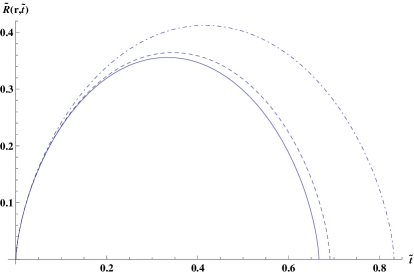
Figure 1: Areal radius $\tilde{R}(r,\tilde{t})$ as a function of time $\tilde{t}$ for $r/r_{c}=0$ (solid line), $0.2$ (dashed line) and $0.5$ (dot-dashed line).

Interestingly, the presence of a density perturbation in our example of an EdS universe, even when initially localized, makes the whole universe to eventually collapse. For instance, a region with a comoving radius of $r=2r_{c}$ collapses at $\tilde{t}=34.1$. Therefore, the expansion rate of the universe at this radius is slightly different from the background EdS.

In Fig.(2) we show the initial instants of the evolution of the profile of the density contrast $\delta(r,\tilde{t})$. The behavior of the perturbation near the sharp boundary is a consequence of numerical instabilities that do not appear in the exact solution.

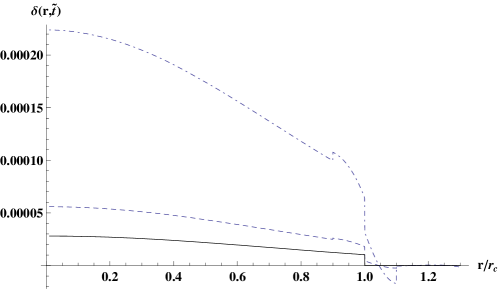
Figure 2: Density contrast $\delta(r,\tilde{t})$ as a function of comoving radius in units of $r_{c}$ for the initial contrast (solid line), density contrast at $\tilde{t}=10^{-7}$ (dashed line) and $\tilde{t}=10^{-6}$ (dot-dashed line).

When one is still in the linear regime, the shape of the profile does not change significantly. For times close to the collapse of the center, the density profiles approach Gaussian profiles with different widths, as shown in Fig.(3).

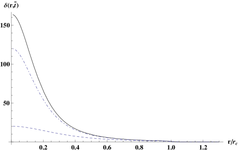
Figure 3: Density contrast $\delta(r,\tilde{t})$ as a function of comoving radius in units of $r_{c}$ for $\tilde{t}=0.5$ (dashed line), density contrast at $\tilde{t}=0.60$ (dot-dashed line) and $\tilde{t}=0.61$ (solid line).

III.2 $\Lambda$CDM background

We now proceed to study the evolution of an inhomogeneous spherical density perturbation in a background with dark matter and cosmological constant, where $\overline{\rho}\left(t\right)=\frac{\overline{\rho}_{m}^{0}}{a^{3}}+\rho_{\Lambda}$ and $\Omega_{m}^{0}+\Omega_{\Lambda}^{0}=1$.

As the cosmological constant is not perturbed, it only affects the behavior of the density contrast through changing the evolution of $a\left(t\right)$ and $\widetilde{R}\left(r,t\right)$. We solve the LTB equations with a cosmological constant, assuming that at an arbitrary initial time $t_{i}=0$, the whole universe follows the background expansion with $R(r,t_{i})=a(t_{i})r$ but it has an initial small density perturbation specified by the profile $g(r)$.

The function mass $m(r)$ now becomes

$$m\left(r\right)=\frac{1}{2}H_{0}^{2}\Omega_{m}^{0}r^{3}h\left(r\right)\,.$$ (43)

Using time in units of the Hubble age today and distance in units of the comoving radius, we will solve the acceleration equation

$$\frac{\partial^{2}\widetilde{R}}{\partial\widetilde{t}^{2}}=-\frac{1}{2}\Omega_{m}^{0}\widetilde{R}^{-2}h\left(r\right)+\Omega_{\Lambda}^{0}\widetilde{R}$$ (44)

for a given value of $r$ and initial conditions

$$\left(\frac{\partial\widetilde{R}}{\partial\widetilde{t}}\right)_{i}=\sqrt{\frac{\Omega_{m}^{0}}{a_{i}}+\Omega_{\Lambda}^{0}a_{i}^{2}}$$ (45)

and $\widetilde{R}_{i}=a_{i}$. In our example below we will use $\Omega_{m}^{0}=0.23$ and $\Omega_{\Lambda}^{0}=0.77$, in which case $\tilde{t}=1.037$ today.

We should point out that also in this case there are exact solutions in terms of implicit Weierstrass-p functions for which the implementation has to be carried semi-analytically 1965PNAS…53….1O . Since this implementation is perhaps as intricate as solving the equations numerically, we have opted for the latter procedure, for simplicity.

In Fig. (4) we show that the time evolution of $\tilde{R}(r,t)$ has the same qualitative behavior as in the EdS case, except that from a certain radius on (around $r=0.7r_{c}$ in our example) the effect of the cosmological constant halts the collapse. This is in agreement with the recent analysis of Mimoso:2009wj , where it was found a dividing shell separating expanding and collapsing regions in general models.

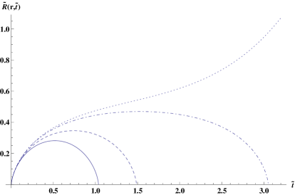
Figure 4: Areal radius $\tilde{R}(r,\tilde{t})$ as a function of time $\tilde{t}$ for $r/r_{c}=0.01$ (solid line), $0.5$ (dashed line), $0.7$ (dot-dashed line) and $0.75$ (dotted line).

The initial evolution of perturbations in matter is shown in Fig.(5). Again we show the initial instants of the evolution of the profile of the density contrast $\delta(r,\tilde{t})$. The small bump around $r=r_{c}$ is due to numerical instabilities and appears because of the sharp boundary in the density profile. Notice that the perturbation profile rapidly evolves to a Gaussian in the nonlinear regime, as can be seen in Fig.(6).

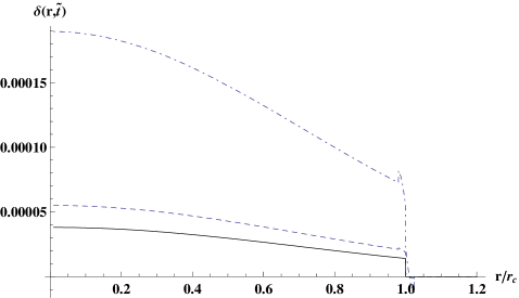
Figure 5: Density contrast $\delta(r,\tilde{t})$ as a function of comoving radius in units of $r_{c}$ for the initial contrast (solid line), density contrast at $\tilde{t}=10^{-7}$ (dashed line) and $\tilde{t}=10^{-6}$ (dot-dashed line).

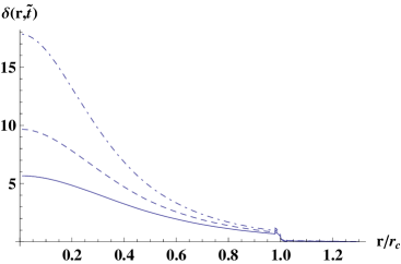
Figure 6: Density contrast $\delta(r,\tilde{t})$ as a function of comoving radius in units of $r_{c}$ at $\tilde{t}=0.5$ (solid line), $\tilde{t}=0.6$ (dashed line) and $\tilde{t}=0.7$ (dot-dashed line).

IV Conclusion

In this work we have implemented a simple generalization of the spherical top-hat collapse model including a general initial profile for the perturbation. We compute the nonlinear evolution of the density perturbation. We chose as an example a simple Gaussian profile with a sharp cutoff that separates the perturbed region from the background. We showed that the density perturbations evolve differently in an EdS and a $\Lambda$CDM background, where in the latter case there is a dividing shell between an expansion and a contraction region inside the perturbation. One should notice that from the usual definition of the quantity $\delta_{c}(z)$, which is the linearly evolved density contrast with an initial condition such that the nonlinear collapse occurs at a redshift $z$, that its value in principle depends only on the background cosmology, being independent of the density profile.

We plan to extend our method to more realistic models including interacting fluids with pressure, where no closed form solutions can be obtained.

References

References

- (1) Dark Energy Survey, T. Abbott et al., (2005), astro-ph/0510346, http://www.darkenergysurvey.org/.
- (2) LSST, J. A. Tyson, Proc. SPIE Int. Soc. Opt. Eng. 4836, 10 (2002), astro-ph/0302102, http://www.lsst.org/lsst,.
- (3) The EUCLID team, T. E. team, (2008), http://sci.esa.int/science-e/www/area/index.cfm?fareaid=102.
- (4) J. M. Bardeen, Phys. Rev. D22, 1882 (1980).
- (5) H. Kodama and M. Sasaki, Prog. Theor. Phys. Suppl. 78, 1 (1984).
- (6) J. E. Gunn and I. Gott, J. Richard, Astrophys. J. 176, 1 (1972).
- (7) T. Padmanabhan, (1993).
- (8) P. Fosalba and E. Gaztanaga, Mon. Not. Roy. Astron. Soc. 301, 503 (1998), astro-ph/9712095.
- (9) W. H. Press and P. Schechter, Astrophys. J. 187, 425 (1974).
- (10) M. C. Martino, H. F. Stabenau, and R. K. Sheth, Phys. Rev. D79, 084013 (2009), 0812.0200.
- (11) F. Schmidt, M. V. Lima, H. Oyaizu, and W. Hu, Phys. Rev. D79, 083518 (2009), 0812.0545.
- (12) F. Schmidt, W. Hu, and M. Lima, Phys. Rev. D81, 063005 (2010), 0911.5178.
- (13) D. F. Mota and C. van de Bruck, Astron. Astrophys. 421, 71 (2004), astro-ph/0401504.
- (14) N. J. Nunes and D. F. Mota, Mon. Not. Roy. Astron. Soc. 368, 751 (2006), astro-ph/0409481.
- (15) N. J. Nunes, A. C. da Silva, and N. Aghanim, Astron. Astroph. 450, 899 (2006), astro-ph/0506043.
- (16) C. Horellou and J. Berge, Mon. Not. Roy. Astron. Soc. 360, 1393 (2005), astro-ph/0504465.
- (17) M. Manera and D. F. Mota, Mon. Not. Roy. Astron. Soc. 371, 1373 (2006), astro-ph/0504519.
- (18) B. M. Schaefer and K. Koyama, Mon. Not. Roy. Astron. Soc. 385, 411 (2008), 0711.3129.
- (19) L. R. Abramo, R. C. Batista, L. Liberato, and R. Rosenfeld, JCAP 0711, 012 (2007), arXiv:0707.2882 [astro-ph].
- (20) L. R. Abramo, R. C. Batista, L. Liberato, and R. Rosenfeld, Phys. Rev. D79, 023516 (2009), 0806.3461.
- (21) S. Basilakos, J. C. Bueno Sanchez, and L. Perivolaropoulos, Phys. Rev. D80, 043530 (2009), 0908.1333.
- (22) F. Pace, J. C. Waizmann, and M. Bartelmann, (2010), 1005.0233.
- (23) N. Wintergerst and V. Pettorino, (2010), 1005.1278.
- (24) P. Brax, R. Rosenfeld, and D. A. Steer, (2010), 1005.2051.
- (25) J. Plebanski and A. Krasinski, Cambridge, UK: Univ. Pr. (2006) 534 p.
- (26) G. Lemaitre, Gen. Rel. Grav. 29, 641 (1997).
- (27) R. C. Tolman, Proc. Nat. Acad. Sci. 20, 169 (1934).
- (28) H. Bondi, Mon. Not. Roy. Astron. Soc. 107, 410 (1947).
- (29) E. W. Kolb, S. Matarrese, and A. Riotto, New J. Phys. 8, 322 (2006), astro-ph/0506534.
- (30) K. Enqvist, Gen. Rel. Grav. 40, 451 (2008), 0709.2044.
- (31) J. Garcia-Bellido and T. Haugboelle, JCAP 0804, 003 (2008), 0802.1523.
- (32) A. Paranjape and T. P. Singh, JCAP 0803, 023 (2008), 0801.1546.
- (33) G. C. Omer, Proceedings of the National Academy of Science 53, 1 (1965).
- (34) J. P. Mimoso, M. Le Delliou, and F. C. Mena, Phys. Rev. D81, 123514 (2010), 0910.5755.