Neutral skyrmion configurations in the low-energy effective theory of spinor condensate ferromagnets

Abstract

We study the low-energy effective theory of spinor condensate ferromagnets for the superfluid velocity and magnetization degrees of freedom. This effective theory describes the competition between spin stiffness and a long-ranged interaction between skyrmions, topological objects familiar from the theory of ordinary ferromagnets. We find exact solutions to the non-linear equations of motion describing neutral configurations of skyrmions and anti-skyrmions. These analytical solutions provide a simple physical picture for the origin of crystalline magnetic order in spinor condensate ferromagnets with dipolar interactions. We also point out the connections to effective theories for quantum Hall ferromagnets.

I Introduction

For systems with broken symmetries, low-energy effective theories provide a simple and powerful tool for describing the relevant physics. The focus is on the long-wavelength Goldstone modes which emerge from the microscopic degrees of freedom. This often reveals the connections between seemingly unrelated systems that share the same pattern of symmetry breaking. The most well-known example is that of the complex scalar field used in the low-energy theories of bosonic superfluids Gross (1961); Pitaevskii (1961), fermionic superconductors Ginzburg and Landau (1950), and XY spin systems Kosterlitz and Thouless (1973).

Effective theories also bring to light subtle topological effects that may become important at low energies. Goldstone modes often carry a non-trivial topology which can give rise to the appearance of topological defects. For example, in two spatial dimensions Kosterlitz and Thouless pointed out the crucial role of vortices for the complex scalar field Kosterlitz and Thouless (1973); Minnhagen (1987). Vortices are point-like topological defects around which the phase of the complex scalar field winds by an integer multiple of $2\pi$.

Ultracold atomic systems provide an ideal testing ground for low-energy effective theories. The microscopic degrees of freedom are well-isolated from the environment experimentally and well-understood theoretically. The challenge is in describing how these microscopic degrees of freedom organize at low energies in the presence of non-trivial interactions. When only one internal hyperfine level is important, the phenomenon of scalar Bose-Einstein condensation is given by the low-energy theory of the complex scalar field Pitaevskii and Stringari (2003); Pethick and Smith (2001); Ozeri et al. (2005). A series of ground breaking experiments have observed vortex lattices in rotating condensates Matthews et al. (1999); Abo-Shaeer et al. (2001) as well as evidence for the role of vortices in the equilibrium Kosterlitz-Thouless transition for two-dimensional condensates Hadzibabic et al. (2006).

For ultracold atoms with a complex internal level structure, there are various patterns of symmetry breaking. This lead to rich possibilities and challenges for low-energy effective descriptions. Spinor condensate ferromagnets are one such system which has seen a number of important experimental advancements (see Ref. Stamper-Kurn and Ketterle (2000)). This includes the development of optical dipole traps used for preparation Stamper-Kurn et al. (1998) and phase-contrast imaging used for detection Higbie et al. (2005) in $S=1$ ⁸⁷Rb. In addition to the phase degree of freedom familiar from single-component condensates, the magnetization naturally arises as a description of the low-energy spin degrees of freedom. A vector quantity sensitive to both the population and coherences between the three hyperfine levels, the magnetization can be directly imaged in experiments Higbie et al. (2005).

One of the most striking observations in spinor condensate ferromagnets is the spontaneous formation of crystalline magnetic order Vengalattore et al. (2008, 2009). From an initial quasi-two-dimensional condensate prepared with a uniform magnetization, a crystalline lattice of spin domains emerges spontaneously at sufficiently long times. The presence of a condensate with magnetization spontaneously breaks global gauge invariance and spin rotational invariance. Additionally, crystalline order for the magnetization breaks real space translational and rotational symmetry. Previous works have pointed out the crucial role of dipolar interactions in driving dynamical instabilities within the uniform condensate towards states with crystalline order Cherng and Demler (2009); Kawaguchi et al. (2009); Sau et al. (2009). Numerical analysis of the full multi-component Gross-Pitaevskii equations suggest dipolar interactions can give rise to states with crystalline order Kawaguchi et al. (2009); Zhang and Ho (2009).

In this and a companion paper Levitov et al. (2010), we take a complementary approach and focus on the low-energy effective theory of two-dimensional spinor condensate ferromagnets. This effective theory describes the interaction between the superfluid velocity and the magnetization degrees of freedom. Previous work has derived the equations of motion for this effective theory Lamacraft (2008); Barnett et al. (2009). We extend this result to demonstrate how the Lagrangian for the effective theory can be written as a non-linear sigma model in terms of the magnetization alone. The effect of the superfluid velocity is to induce a long-ranged interaction term between skyrmions, topological defects familiar from the theory of ordinary ferromagnets Rajaraman (1982). In contrast to the point-like topological defects of vortices, skyrmions describe extended magnetization textures which carry a quantized topological charge.

In the companion paper Levitov et al. (2010), we study how symmetry groups containing combined real space translational, real space rotational, and spin space rotational symmetry operations can be used to classify possible crystalline magnetic orders. Within each symmetry class, we find minimal energy configurations describing non-trivial crystalline configurations.

The main purpose of this paper is to give a simple physical physical picture for the origin of crystalline order in terms of neutral configurations of skyrmions and anti-skyrmions. Long-ranged skyrmion interactions force magnetization configurations to have net neutral collections of topological defects. We show this explicitly by finding exact analytical solutions for the non-linear equations of motion describing both localized collections of skyrmions and anti-skyrmions as well as extended skyrmion and anti-skyrmion stripes.

Skyrmions have non-trivial spin configurations that spontaneously break translational and rotational invariance in real space. Proposed originally in high energy physics as a model for mesons and baryons Skyrme (1962); Klebanov (1985), skyrmions have found applications in a number of diverse fields including quantum hall ferrogmagnets Sondhi et al. (1993); Brey et al. (1995), and magnetically ordered crystals Bogdanov and Yablonskii (1989); Muhlbauer et al. (2009); Neubauer et al. (2009); Münzer et al. (2010).

A neutral collection of such topological objects is able to take advantage of the dipolar interaction energy without a large penalty in the skyrmion interaction energy. Since a neutral skyrmion configuration has the same topological number as the uniform magnet, its stability is not ensured by topology alone. However, the scale invariance of the skyrmion interaction energy rules out the most straightforward instability of bringing skyrmions and anti-skyrmions closer together. Essentially, the skyrmion interaction energy forces the charge densities of a skyrmion and anti-skyrmion pair to shrink as the distance between them shrinks so that the overall energy remains the same.

The analytical solutions we find without dipolar interactions closely resemble the minimal energy configurations found numerically in the presence of dipolar interactions. The role of dipolar interactions can then be seen as stabilizing these non-trivial solutions of the effective theory. We point out that magnetic dipolar interactions are small. Thus it is a good starting point to find states which are static nontrivial solutions of the system without dipolar interactions.

The effective theory of spinor condensate ferromagnets is essentially identical to that of the quantum Hall ferromagnets Sondhi et al. (1993); Lee and Kane (1990). Although the microscopic degrees of freedom are fermionic electrons, the magnetization order parameter is bosonic. The Coloumb interaction between electrons then gives a contribution to the skyrmion interaction for the effective theory. The resulting skyrmion interaction is qualitatively the same as the one for spinor condensate ferromagnets. This suggests the study of spinor condensate ferromagnets may have interesting connections to quantum hall ferromagnets and vice versa.

The plan of this paper is as follows. In Sec. II we review the theory of ordinary ferromagnets and how skyrmion solutions arise from the non-linear Landau-Lifshitz equations of motion. We then proceed to review how these skyrmion solutions are used in the low-energy effective theory of quantum Hall ferromagnets in Sec. III. Next we derive the low-energy effective theory for spinor condensate ferromagnets in Sec. IV. In particular, we demonstrate how a long-ranged skyrmion interaction term (which also appears for quantum hall ferromagnets) arises from coupling of the magnetization to the superfluid velocity.

In Sec. V, we discuss how to interpret the mathematical structure of skyrmion solutions for ordinary ferromagnets in terms of a separation of variables. This approach allows us to use find new exact solutions for the oridinary ferromagnet. More importantly, it also allows us to generalize the skyrmion solutions of the ordinary ferromagnet to find analytical solutions for the spinor condensate ferromagnet. These latter solutions describe both neutral collections of localized skyrmions and anti-skyrmions as well as extended stripe configurations. Finally, we discuss how the analytical solutions we find offer insight into quantum hall ferromagnets and spinor condensate ferromagnets with dipolar interactions in Sec. VI

II Skyrmions in ferromagnets

We begin by reviewing the theory of ordinary two-dimensional ferromagnets described by the following Lagrangian, Hamiltonian, and Landau-Lifshitz equations of motion Fradkin (1991)

$$\mathcal{L} =-S\int dtd^{2}x\mathcal{A}(\hat{n})\cdot\partial_{t}\hat{n}-\int dt\mathcal{H}$$

$$\mathcal{H} =\frac{S}{4}\int d^{2}x\nabla(\hat{n})^{2}$$

$$\partial_{t}\hat{n} =\frac{1}{2}\hat{n}\times\nabla^{2}\hat{n}$$ (1)

where $\hat{n}$ is a three component real unit vector and $\mathcal{A}(\hat{n})$ is the unit monopole vector potential. The order parameter $\hat{n}$ describes the magnetization and is a unit vector living on the sphere. Calculating the variation of the Lagrangian to derive the Landau-Lifshitz equations Stone (1989, 1996) can be done by using $\delta\hat{n}=\delta w\times\hat{n}$. This is consistent with the constraint $|\hat{n}|=1$ since $\delta\hat{n}\cdot\hat{n}=0$ by construction. The variation of the term $\int dt\mathcal{A}(\hat{n})\cdot\partial_{t}\hat{n}$ is clearest when using its geometric interpretation as the area on the sphere swept by $\hat{n}$. While we include time dependent terms for completeness, in this paper we will only consider static solutions

In addition to the trivial uniform solution, there are non-trivial soliton solutions to the Landau-Lifshitz equations called skyrmions. By parameterizing

$$\hat{n}=\begin{bmatrix}\sin(\alpha)\cos(\beta)&\sin(\alpha)\sin(\beta)&\cos(\alpha)\end{bmatrix}^{T}$$ (2)

we see $\alpha$ controls $\hat{n}_{z}$, the $\hat{z}$ component of the magnetization while $\beta$ controls the canonically conjugate variable giving the orientation of $\hat{n}_{x}$, $\hat{n}_{y}$, the $\hat{x}$, $\hat{y}$ components of the magnetization.

The minimal energy solutions within each topological sector are called skyrmions and can be written in the form Rajaraman (1982)

$$\tan(\alpha/2)e^{i\beta}=\exp[f(x+iy)]=\exp[u(x,y)+iv(x,y)]$$ (3)

where $f(z)$ is a holomorphic function of $z$ with real part $u(x,y)$ and imaginary part $v(x,y)$. The function $f(z)\sim n\log(z-z_{0})$ can have logarithmic singularities . Since $\beta$ has to be $2\pi$ periodic, the residues of these singularities must be integers. This implies $\exp[f(x+iy)]$ can only have zeros or poles. The resulting spin configuration has $\hat{n}_{z}=+1$ ($\hat{n}_{z}=-1$) at zeros (poles) of $\exp[f(z)]$ while $\hat{n}_{x}$, $\hat{n}_{y}$ wind anti-clockwise (clockwise) along a path circling the zeros (poles) in a anti-clockwise direction.

These solutions describe topological defects of ordinary ferromagnets. For fixed boundary conditions, smooth, finite energy configurations are separated into distinct classes characterized by a quantized topological invariant $\int d^{2}xq(x)=4\pi N$ where $N$ is the number of times $\hat{n}$ covers the sphere. Here

$$q=\epsilon_{\mu\nu}\hat{n}\cdot\nabla_{\mu}\hat{n}\times\nabla_{\nu}\hat{n}$$ (4)

is the skyrmion density which is positive for $f(z)$ holomorphic. From here on, lower Greek indices (upper Roman indices) refer to real space (order parameter) components.

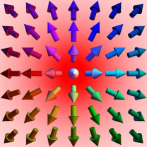
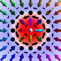
Figure 1: A single localized skyrmion carrying $4\pi$ net skyrmion charge in the ordinary ferromagnet (left). Neutral configuration consisting of a localized skyrmion carrying $+4\pi$ skyrmion charge in a negative background carrying $-4\pi$ skyrmion charge in the spinor condensate ferromagnet (right). Notice the $+\hat{z}$ ($-\hat{z})$ meron carrying $+2\pi$ ($+2\pi$) net skyrmion charge at the origin (at infinity) for the ordinary ferromagnet are mapped to a skyrmion (anti-skyrmion) carrying $+4\pi$ (-$4\pi$) net skyrmion charge in the spinor condensate ferromagnet. Red (blue) background indicates positive (negative) skyrmion density $q$, black 2D arrows the superfluid velocity $\mathbf{v}$ for the spinor condensate ferromagnet, and shaded 3D arrows the magnetization $\hat{n}$.

Consider the single skyrmion solution shown in the left of Fig. 1. It corresponds to $f(z)=\log(z)$, carries net skyrmion charge $4\pi$, and can be decomposed into a $+\hat{z}$ meron at the origin and a $-\hat{z}$ meron at infinity. Essentially, a meron can be thought of as half of a skyrmion and characterized by two signed quantities: the direction of the magnetization at the core and the orientation of the winding away from the core. The sign of the skyrmion density is the product of the sign of these two quantities. For example, the $+\hat{z}$ meron at the origin to the left of Fig. 1 carries net skymrion charge $2\pi$.

For spinor condensate ferromagnets, scale invariance of the skyrmion interaction term guarantees stability against trivial rescaling. However, this may change if we introudce a short distance cutoff or quantum fluctuations.

Notice the Lagrangian in Eq. 1 has translational, rotational, and scale invariance in real space as well as rotational invariance in spin space. The single skyrmion solution spontaneously breaks all of these symmetries. However, the action is invariant for $f(z)=\log[f_{0}(z-z_{0})]$ with complex constants $z_{0}$ and $f_{0}$. Taking solutions with $z_{0}\neq 0$ corresponds to spatially translating the solution with $z_{0}=0$, solutions with $\text{Re}[f_{0}]\neq 1$ correponds to spatially rescaling the the solution with $f_{0}=1$, and solutions with $\text{Im}[f_{0}]\neq 0$ corresponds to rotation of the $f_{0}=1$ solution. In addition, the action is the same for $O\hat{n}$ where $O$ is a rotation matrix describing solutions related by spin space transformations.

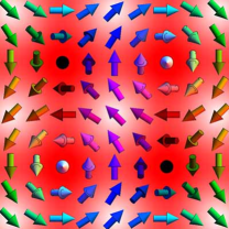
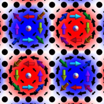
Figure 2: Unit cell for a lattice of localized skyrmions carrying $8\pi$ net skyrmion charge per unit cell in the ordinary ferromagnet (left). Unit cell for a neutral configuration carrying zero net skyrmion charge per unit cell in the spinor condensate ferromagnet (right). Notice $+\hat{z}$ ($-\hat{z})$ merons are mapped to skyrmions (anti-skyrmions). Red (blue) background indicates positive (negative) skyrmion density $q$, black 2D arrows the superfluid velocity $\mathbf{v}$, and shaded 3D arrows the magnetization $\hat{n}$.

Collections of multiple skyrmions are described by $f(z)$ having multiple singularities. A square lattice of skyrmions with net skyrmion charge $8\pi$ per unit cell is shown in the left of Fig. 2. It can also be decomposed into a collection of two $+\hat{z}$ merons and two $-\hat{z}$ merons arranged antiferromagnetically. In addition, there are solutions $\tan(\alpha/2)e^{i\beta}=\exp[f(x-iy)]$ with $f(\bar{z})$ antiholomorphic characterized by $\hat{x}$, $\hat{y}$ components winding in the opposite direction compared to holomorphic solutions and $q$ negative.

III Quantum Hall Ferromagnets

After describing the structure of skyrmion solutions for ordinary ferromagnets, we now briefly review how they are used in the study of quantum Hall ferromagnets Sondhi et al. (1993); Lee and Kane (1990). For the low-energy effective theory of quantum Hall ferromagnets, spin $1/2$ electrons in a magnetic field are described by a two component Chern-Simons composite boson theory. The bosons couple to the physical gauge field due to the magnetic field and a fictitious Chern-Simons gauge field which attaches appropriate flux quanta to change from bosonic to fermionic statistics. At appropriate filling fractions, the physical and Chern-Simons fluxes cancel and the resulting quantum Hall plateau is described as a condensate of composite bosons.

The Lagrangian and Hamiltonian for the resulting effective theory is given by

$$\mathcal{L}= -\frac{1}{2}\int dtd^{2}x\mathcal{A}(\hat{n})\cdot\partial_{t}\hat{n}-\int dt\mathcal{H}$$

$$\mathcal{H}= \int d^{2}x\left[\frac{1}{8}(\nabla\hat{n})^{2}+\frac{1}{2}\vec{B}\cdot\hat{n}\right]$$

$$+\frac{1}{8}\int d^{2}xd^{2}y[q(x)-\bar{q}]G(x-y)[q(y)-\bar{q}]$$ (5)

where $\vec{B}$ is the magnetic field giving rise to a linear Zeeman shift, $q(x)$ is the skyrmion density and $\bar{q}=\int d^{2}xq(x)$ is the net skyrmion charge.

The coupling of the bosons to the Chern-Simons field gives rise to the skyrmion interaction term. At long distances, the Chern-Simons field ties the skyrmion density to the deviation of the physical electron density from its background value. In fact skyrmions are lowest energy quasiparticles at a filling factor of one Sondhi et al. (1993); Fertig et al. (1994). Thus, the skyrmion density inherits the Coloumb interaction for the electron density. Away from quantum Hall plateaus, the background value $\bar{q}$ is non-zero and the singular $|x-y|^{-1}$ behavior in $G(x-y)$ forces finite energy configurations to have non-zero net skyrmion charge.

Thus the focus is on static configurations carrying net skyrmion charge. The skyrmion solutions of the ordinary ferromagnet have non-zero $\bar{q}$ and provide a good qualitative description of quantum Hall ferromagnets away from quantum Hall plateaus. For example, a sqaure lattice of skyrmions as shown in Fig. 2 carries a net charge of $8\pi$ per unit cell and can be used as a starting point for studying configurations carrying finite $\bar{q}$. Although such solutions take into account the spin stiffness and the long-ranged divergence of the skyrmion interaction, quantitative results require additional analysis arising from the detailed form of skyrmion interaction and the linear Zeeman shift. This usually involves numerical minimization Fertig et al. (1997); Lejnell et al. (1999); Fertig et al. (1994); Timm et al. (1998) of the Hamiltonian in Eq. 5.

IV Spinor Condensate Ferromagnets

Having reviewed known results on ordinary and quantum Hall ferromagnets, we now consider spin $S$ spinor condensate ferromagnets described by the microscopic condensate wavefunction $\mathbf{\Psi}$, a $2S+1$ complex vector Ohmi and Machida (1998); Ho (1998). The microscopic Gross-Pitaevskii Lagrangian is given by

$$\mathcal{L} =\int dti\mathbf{\Psi}^{\dagger}\partial_{t}\mathbf{\Psi}-\int dt\mathcal{H}-\int dt\mathcal{H}_{S}$$

$$\mathcal{H} =\int d^{2}x\left[\frac{1}{2m}|\nabla\mathbf{\Psi}|^{2}+g_{0}(\mathbf{\Psi}^{\dagger}\mathbf{\Psi})^{2}+g_{s}(\mathbf{\Psi}^{\dagger}\vec{F}\mathbf{\Psi})^{2}\right]$$ (6)

where $\vec{F}$ are spin matrices and $g_{0}>0$ gives the spin-independent contact interaction strength while $g_{s}<0$ gives the spin-dependent contact interaction strength which favors finite magnetization. Here, $\mathcal{H}_{S}$ denotes additional spin dependent interactions such as the quadratic Zeeman shift and dipolar interactions.

As was the case for quantum Hall ferromagnets, we expect a simpler description to emerge at low energies. The resulting low-energy effective theory should only involve the condensate phase $\phi$ and local magnetization $\hat{n}$ which describe the order parameters of the system. Previous work has shown this can be done at the level of the equations of motion Lamacraft (2008). In this section, we extend this result to derive the Lagrangian and Hamiltonian for the effective theory solely in terms of the magnetization. However, the skyrmion density acts as a source of voriticity for the superfluid velocity. Thus, the effect of the superfluid phase is to induce a logarithmic vortex-vortex interaction between skyrmions. The resulting non-linear sigma model is essentially identical to that of the quantum Hall ferromagnet but with skyrmion interaction $G(x-y)\sim\log(x-y)$ having logarithmic behavior instead of $|x-y|^{-1}$ behavior.

We begin by considering energies below the scale of spin-independent $g_{0}$ and ferromagnetic spin-dependent $g_{s}$ contact interactions. The condensate has fixed density $\mathbf{\Psi}^{\dagger}\mathbf{\Psi}=\rho$ and fully polarized magnetization $\mathbf{\Psi}^{\dagger}\vec{F}\mathbf{\Psi}=S\rho\hat{n}$ where $\vec{F}$ are spin matrices. The states that satisfy these constraints are parameterized solely in terms of the low-energy degrees of freedom

$$\mathbf{\Psi} =\sqrt{\rho}e^{i\phi}\psi_{\hat{n}}, \hat{n}\cdot\vec{F}\psi_{\hat{n}} =S\rho\psi_{\hat{n}}$$ (7)

where $\phi$ descrribes the phase of the condensate and $\psi_{\hat{n}}$ is a fully polarized unit spinor with $\hat{n}$ describing the orientation of the magnetization. Although $\phi$ is not directly observable, the superfluid velocity is a physical quantity

$$\mathbf{v}_{\mu}=\nabla_{\mu}\phi-i\psi_{\hat{n}}^{\dagger}\nabla_{\mu}\psi_{\hat{n}}$$ (8)

which has contributions from both $\phi$ and $\psi_{\hat{n}}$.

In this paper, we are primarily interested in the competition between the spin stiffness and superfluid kinetic energy. In the companion paper Levitov et al. (2010), we address the effect of magnetic dipolar interactions. From here on, we consider the case $\mathcal{H}_{S}=0$. From the Gross-Pitaevskii Lagrangian in Eq. 6, the Berry’s phase term becomes $i\mathbf{\Psi}^{\dagger}\partial_{t}\mathbf{\Psi}=-\rho\partial_{t}\phi-S\rho\mathcal{A}(\hat{n})\cdot\partial_{t}\hat{n}$ while the kinetic energy term is given by $|\nabla\mathbf{\Psi}|^{2}=S\rho/2(\nabla\hat{n})^{2}+\rho\mathbf{v}^{2}$ and the interaction terms give constants. This gives the Lagrangian and Hamiltonian as

$$\mathcal{L} =-S\int dtd^{2}x\mathcal{A}(\hat{n})\cdot\partial_{t}\hat{n}-\int dt\mathcal{H}$$

$$\mathcal{H} =\int d^{2}x\left[\frac{S}{4}(\nabla\hat{n})^{2}+\frac{1}{2}\mathbf{v}^{2}\right]$$ (9)

where we take $\rho=m=1$ for simplicity. Notice for fixed $\rho$, the $\partial_{t}\phi$ term is a total derivative which we exclude. Compared to the Lagrangian describing ordinary ferromagnets in Eq. 1, there is an additional superfluid kinetic energy term $\mathbf{v}_{\mu}\mathbf{v}_{\mu}$.

The global phase $\phi$ enters the Lagrangian quadratically and only through $\mathbf{v}$. The equation of motion for $\phi$ gives $\nabla_{\mu}\mathbf{v}_{\mu}=0$ implying the superfluid velocity is divergenceless. This follows from $\mathbf{v}$ describing transport of the density $\rho$, a conserved quantity which is locally fixed at low energies due to the spin-independent contact interaction. This implies that $\mathbf{v}_{\mu}\mathbf{v}_{\mu}$ only depends on the divergenceless part of $\mathbf{v}$. In momentum space, this is $\mathbf{v}_{\mu}(+k)[\delta_{\mu\nu}-k_{\mu}k_{\nu}/k^{2}]\mathbf{v}_{\nu}(-k)$ which can also be written as $F_{\mu\nu}(+k)F_{\mu\nu}(-k)/2k^{2}$.

Here we have introduce the analog of the field strength tensor $F_{\mu\nu}=\nabla_{\mu}\mathbf{v}_{\nu}-\nabla_{\nu}\mathbf{v}_{\mu}$, a local quantity that depends only on the divergenceless part of $\mathbf{v}$. In two dimensions, there is only one non-zero component to $F_{\mu\nu}$. From Eq. 8, this is given by the skyrmion density $F_{xy}=-F_{yx}=Sq$. Here we assume that the condensate phase $\phi$ does not contribute to $F_{xy}$ through vortex-like singularities. This is valid because the vortex core energy is large.

The above results give $\mathbf{v}$ solely in terms of $\hat{n}$ as

$$\nabla_{\mu}\mathbf{v}_{\mu} =0, \epsilon_{\mu\nu}\nabla_{\mu}\mathbf{v}_{\nu} =Sq$$ (10)

with $q$ the skyrmion density. Gradients in the order parameter $\hat{n}$ arise in part from phase gradients in the condensate wavefunction $\mathbf{\Psi}$. Topologically non-trivial magnetization configurations can thus give rise to vorticity described by a non-zero curl $\epsilon_{\mu\nu}\nabla_{\mu}\mathbf{v}_{\nu}\neq 0$.

By introducing the two-dimensional logarithmic Green’s function $-\nabla^{2}G(x)=\delta(x)$ we can write the superfluid kinetic energy $F_{\mu\nu}(+k)F_{\mu\nu}(-k)/2k^{2}$ in real space and obtain

$$\mathcal{L} =-S\int dtd^{2}x\mathcal{A}(\hat{n})\cdot\partial_{t}\hat{n}-\int dt\mathcal{H}$$

$$\mathcal{H} =\frac{S}{4}\int d^{2}x(\nabla\hat{n})^{2}+\frac{S^{2}}{2}\int d^{2}xd^{2}yq(x)G(x-y)q(y)$$ (11)

with the corresponding equations of motion given by

$$\left(\partial_{t}+\mathbf{v}_{\mu}\nabla_{\mu}\right)\hat{n} =\frac{1}{2}\hat{n}\times\nabla^{2}\hat{n}$$ (12)

along with Eq. 10 for the superfluid velocity solved by

$$\mathbf{v}_{\mu} =S\epsilon_{\mu\nu}\nabla_{\nu}\Phi, -\nabla^{2}\Phi =q$$ (13)

where $\Phi(x)=\int d^{2}xG(x-y)q(y)$ has the interpretation of the two-dimensional Coloumb potential associated with $q$.

Compared to the Landau-Lifshitz equations describing ordinary ferromagnets in Eq. 1, the replacement $\partial_{t}\rightarrow\partial_{t}+\mathbf{v}_{\mu}\nabla_{\mu}$ describes the advection of the magnetization by the superfluid velocity Lamacraft (2008). This advective term arise from variation of the superfluid kinetic energy term in Eq. 9 or equivalently from the skyrmion interaction term in Eq. 11. Recall that we include the time dependence for completeness and focus only on static solutions.

The skyrmion density $q$ gives the vorticity for the superfluid velocity $\mathbf{v}$. Thus, the second term in the Hamiltonian above gives the pairwise logarithmic interaction energy between vortices. In the thermodynamic limit, the logarithmic divergence of $G(x-y)$ at large distances forces finite energy configurations to have zero net skyrmion density $\int d^{2}xq(x)=0$.

Notice Eq. 11 for spinor condensate and Eq. 5 for quantum hall ferromagnets have the same form. Although $G(x-y)$ behaves as $\log|x-y|$ for the former and $|x-y|^{-1}$ for the latter, both give singular contributions at long wavelengths. However, the important absence of a finite backgroud value $\bar{q}$ in the skyrmion interaction implies configurations for spinor condensate ferromagnets must have zero net skyrmion charge.

V Exact solutions with neutral skyrmion charge

In quantum hall systems density deviations from the incompressible state cause skyrmions. Density fluctuations with zero net average (such as impurities) cause spin textures with zero net skyrmion number. States with non-zero skyrmion number occur away from quantum hall plateaus. Thus the analytical skyrmion solutions carrying net charge for the ordinary ferromagnet offered insight into more complicated case of quantum Hall ferromagnets away from the quantum Hall plateau. For spinor condensate ferromangets, we will show how net neutral solutions with skyrmions and anti-skyrmions without dipolar interactions offer insight into the more complicated case with dipolar interactions.

In this section, we find exact analytical solutions for spinor condensate ferromagnets with logarithmic skyrmion interactions in the absence of dipolar interactions. We study the effect of including dipolar interactions numerically after a symmetry analysis in the companion paper Levitov et al. (2010). The exact solutions we find here greatly resemble the numerical solutions in the companion paper. As we discuss in Sec. VI, the interpretation of the exact solutions in terms of neutral collections of skyrmions and anti-skyrmions offers physical insight into the more complicated numerical solutions of the companion paper.

To find exact solutions with zero net skyrmion charge, it is vital to include to effect of the skyrmion interaction term. Recall it is the long wavelength divergence of this term that forces configurations to have zero net skyrmion charge. Although this cannot be done exactly for $|x-y|^{-1}$ interactions as in quantum hall ferromagnets, it is possible for logarithmic interactions as in spinor condensate ferromagnets. Physically, this is because the logarithmic interaction arises solely from the superfluid kinetic energy which is scale invariant just like the spin stiffness term.

We begin with the parameterization of $\hat{n}$ in Eqs. 2, 3, used in the skyrmion solutions of the ordinary ferromagnet. Notice $\alpha$, $\beta$ provide a set of orthogonal coordinates for the sphere describing the order parameter space of $\hat{n}$. For $f(x+iy)=u(x,y)+iv(x,y)$ holomorphic, $u(x,y)$ and $v(x,y)$ provide a set of orthogonal coordinates for the plane describing real space. So for ordinary ferromagnets, skyrmion solutions are given by $\alpha=2\tan^{-1}(e^{u})$ and $\beta=v$ (see also Eq. 3), which can be understood as a separation of variables.

Notice $\alpha(u)$ is a function of $u$ only while $\beta(v)$ is a function of $v$ only. Each orthogonal coordinate of the order parameter space $\alpha$, $\beta$ is a function of only one orthogonal coordinate of real space $u$, $v$, respectively. The reason why using $u$ and $v$ as coordinates is tractable is because they satisfy the Cauchy-Riemann equations $\partial_{x}u=+\partial_{y}v$, $\partial_{y}u=-\partial_{x}v$. In particular, this implies $\nabla u\cdot\nabla v=0$ meaning countour lines of constant $u$ are perpendicular to countour lines of constant $v$ as required for orthogonal coordinates. In addition, both $\nabla^{2}u=0$ and $\nabla^{2}v=0$ satisfy Laplace’s equation. The above two identities simplify expressions involving $\nabla^{2}$ which arise in the equations of motion. In particular, when changing variables from $(x,y)$ to $(u,v)$, the Laplacian retains its form $\partial_{x}^{2}+\partial_{x}^{2}\propto\partial_{u}^{2}+\partial_{v}^{2}$.

An alternative interpretation of the above separation of variables is as follows. Given an arbitrary configuration for $\hat{n}$, consider the contour lines of constant $\hat{n}_{z}$, the $\hat{z}$ component of the magnetization. For contour lines with $\hat{n}_{z}\neq\pm 1$ that form closed curves, consider the winding number of $\hat{n}_{x}+i\hat{n}_{y}=\sin(\alpha)e^{i\beta}$. For smooth configurations, this is a quantized integer that cannot change between neighboring contours which do not cross $\hat{n}_{z}\neq\pm 1$. This implies the winding number is constant in regions between contours with $\hat{n}_{z}\neq\pm 1$. Label different contours of $\hat{n}_{z}$ by $u$ and the label coordinate along each contour by $v$.

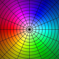
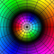
Figure 3: For an arbitrary smooth magnetization configuration, contour lines of $\hat{n}_{z}$ and the phase of $\hat{n}_{x}+i\hat{n}_{y}$ provide a natural coordinate system. For skyrmion solutions of the ordinary ferromanget, this gives an orthogonal coordinate system with contour lines intersecting at right angles. Using the same ansatz for spinor condensate ferromagnets where contour lines intersect at right angles allows us to solve the non-linear and non-local equations of motion. The magnetization and contour lines are shown for the single skyrmion (left) for the ordinary ferromagnet and neutral configuration (right) for the spinor condensate ferromagnet. Hue indicates orientation of $\hat{n}_{x}$, $\hat{n}_{y}$ components of the magnetization and brightness gives the $\hat{n}_{z}$ component with white (black) indicating $\hat{n}_{z}=+1$ ($\hat{n}_{z}=-1$).

In order to have a non-zero winding number, $\beta$ must have some dependence on $v$ and the minimal one is $\beta\propto v$. In principal, $\beta$ can also depend on $u$ and have some non-monotonic dependence on $v$, but linear dependence is the smoothest one compatible with non-zero winding number. We see that skyrmion solutions can be interpreted in the above manner along with the additional condition that $u$ and $v$ are mutually othogonal and satisfy Laplace’s equation. Physically, these additional conditions on $u$ and $v$ can be understood as a consequence of minimizing the spin stiffness. The relationship between contour lines, winding number, and the exact solutions we discussed in this section is shown in Fig. 3.

With this viewpoint, we can now generalize the skyrmion solutions for ordinary ferromagnets and also find new solutions for spinor condensate ferromagnets. For $f(x+iy)=u(x,y)+iv(x,y)$ holomorphic, we take

$$\alpha =\alpha(u), \beta=kv$$ (14)

for the parameterization of Eq. 2. Compared to the skyrmion solutions of Eq. 3 with $\tan(\alpha/2)=\exp[u]$ for ordinary ferromagnets, we allow for general dependence $\alpha(u)$ for spinor ferromagnets. Whereas for ordinary ferromagnets we only need to solve $\nabla^{2}\hat{n}=0$, for spinor condensate ferromagnets we need to solve Eqs. 12, 13 with $\partial_{t}=0$.

In addition, we include a constant of proportionality $\beta=kv$ instead of $\beta=v$. Recall for ordinary ferromagnets, $\beta=+v$ and $f(x+iy)$ holomorphic give skyrmion solutions with positive skyrmion density $q$ while $\beta=-v$ and $f(x-iy)$ antiholomorphic give anti-skyrmion solutions with $q$. We can treat both types of solutions with just $f(x+iy)$ holomorphic by allowing $\beta=kv$ with $k$ positive or negative.

There are two cases to consider for $f(z)$. The first is when $f(z)$ is a polynomial in $z$ with no singularities. This will turn out to describe skyrmion and anti-skyrmion stripe and domain wall configurations for both ordinary and spinor condensate ferromagnets. The second case is when $f(z)$ has singularities. Since $\hat{n}$ should be single-valued, $\beta$ and thus $kv$ can only have constant $2\pi N$ discontinuities with $N$ integer. This implies $f(z)$ can only have logarithmic singularities. These solutions will turn out to simply be the localized skyrmion configurations for ordinary ferromagnets and neutral collections of localized skyrmions and anti-skyrmions for spinor condensate ferromagnets.

Next we consider Eq. 13 for the superfluid velocity $\mathbf{v}$. For the parameterization in Eqs. 2, 14, we see from Eq. 4 that the skyrmion density $q$ only depends on $u$. We thus take $\Phi(u)$ to only depend on $u$ which reduces the equation $-\nabla^{2}\Phi=q$ to $-\Phi^{\prime\prime}(u)=q(u)$. From here on primes denote derivatives with respect to $u$. By solving for $\Phi(u)$ we can then obtain $\mathbf{v}$ by differentiating. Explicitly, we obtain

$$q =-k\cos(\alpha)^{\prime}|\partial_{z}f|^{2}, \mathbf{v}_{z} =iSk[C+\cos(\alpha)]\partial_{z}f$$ (15)

where $\mathbf{v}_{z}=\mathbf{v}_{x}-i\mathbf{v}_{y}$, $\partial_{z}f=\partial_{x}f-i\partial_{y}f$ and $C$ is a constant of integration physically describing a $u$ independent constant contribution to the superfluid velocity.

We now proceed to analyze Eq. 12 for spinor condensate ferromagnets. By substituting the results of Eq. 15 above and the parameterization in Eqs. 2, 14, we find the $\hat{z}$ component of Eq. 12 is automatically satisfied. In addition, the $\hat{x}$ and $\hat{y}$ components are proportional to each other and reduce to a second ordinary differential equation for $\alpha(u)$. For completeness, we can use the same approach to analyze Eq. 1 for ordinary ferromagnets using the same parameterization in Eqs. 2, 3.

For ordinary and spinor condensate ferromagnets, the equations of motion in Eq. 1 and Eq. 12 reduce to

$$2\alpha^{\prime\prime} =+k^{2}\sin(2\alpha)$$

$$2\alpha^{\prime\prime} =-4SCk^{2}\sin(\alpha)-(2S-1)k^{2}\sin(2\alpha)$$ (16)

respectively. Notice the equations of motion for ordinary ferromagnets are formally given by the $S=0$ limit for spinor condensate ferromagnets. Recall the spin stiffness term scales linearly with $S$ whereas the superfluid kinetic energy scales quadratically with $S$. For spinor condensate ferromagnets in the limit $S\rightarrow 0$, the superfluid kinetic energy is negligible compared to the spin stiffness and the ordinary ferromagnet is recovered. From here on, we consider the more general equation of motion for spinor condensate ferromagnets.

Interpreting $u$ as time, this equation is that of a classical particle with coordinate $\alpha$ and momentum $\alpha^{\prime}$. The total energy $E=K+U$ is a constant of motion where $K=(\alpha^{\prime})^{2}/2$ is the kinetic energy while the periodic potential $U$ and equation of motion are

$$U(\alpha) =-2SCk^{2}\cos(\alpha)-\frac{2S-1}{4}k^{2}\cos(2\alpha)$$

$$\alpha^{\prime} =\sqrt{E-U(\alpha)}$$ (17)

with $S=0$ for ordinary ferromagnets. For this type of solution, the total energy calculated from the Hamiltonian in Eq. 11 is given by

$$\mathcal{H} =N\int dudv\frac{S}{2}\left[\frac{2S+1+4C^{2}S}{4}k^{2}-E+\alpha^{\prime 2}\right]$$ (18)

and similarly, $S=0$ for the term in brackets for ordinary ferromagnets.

The integer $N$ comes from changing variables $(x,y)$ to $(u,v)$ and taking into account each $(u,v)$ may occur for multiple $(x,y)$. Mathematically, it is given by the degree of $f$ viewed as a map from the complex plane to itself $\mathbb{C}\rightarrow\mathbb{C}$. For localized skyrmion solutions for the ordinary ferromagnet, it physically corresponds to the skyrmion number. As an example, $f(z)=\log z$ for the solutions shown in Fig. 1 (see Eq. 21 for a generalization) and each value of $(u,v)$ occurs exactly once for $(x,y)$ ranging over the plane and thus $N=1$. For $f(z)=\log[(\vartheta(z-\lambda,i)\vartheta(z-\lambda^{*},i))/(\vartheta(z+\lambda,i)\vartheta(z+\lambda^{*},i))]$ with $\vartheta(z,\tau)$ the elliptic theta function and $\lambda=(1+i)/2$ for the solutions shown in Fig. 2 (see Eq. 22 for a generalization) and each value of $(u,v)$ occurs exactly twice for $(x,y)$ ranging over the unit cell and thus $N=2$.

Here we comment on the significance of the parameters $C$ and $E$. Different values of $C$ and $E$ correspond to solutions with different boundary conditions. Physically, $C$ controls a constant background contribution to the superfluid velocity. The parameter $E$ controls the relative scaling of the two components of the coordinate system. For example, for doubly periodic stripe solutions which we will discuss later, $E$ controls the aspect ratio of the unit cell.

Formally, $E$ and $C$ are constants of integration for the equations of motion. Since Eq. 16 is a second order differential equation, we have to specify both $\alpha(u)$ and $\alpha^{\prime}(u)$, with the latter given indirectly by the constant of motion $E$. In addition, $C$ enters through integration of Eq. 15 relating the skyrmion density to the superfluid velocity.

These considerations mean that the total energy in Eq. 18 cannot be directly compared for different $C$ and $E$. In particular, one should not consider minimizing the total energy $\mathcal{H}$ with respect to $E$ and $C$. Specific values of $E$, and $C$ will be selected by terms beyond the non-linear sigma model considered in this paper.

V.1 Localized skyrmions and anti-skyrmions

We begin by considering the case of localized skyrmions for ordinary ferromagnets and neutral collections of localized skyrmions and anti-skyrmions for spinor condensate ferromagnets. This corresponds to $f(z)$ having logarithmic singularities. The singularities should be of integer magnitude and $k$ should also be an integer.

Requiring a well-behaved, finite energy solution gives rise to several constraints. Consider Eq. 15 for the skyrmion density $q$ and supefluid velocity $\mathbf{v}$. Since $\partial_{z}f$ diverges at the logarithmic singularities, we require $\cos(\alpha)^{\prime}$ and $C+\cos(\alpha)$ to vanish. In addition, a finite region in $(x,y)$ near logarithmic singularities is mapped to an infinite region in $(u,v)$. The constant term in Eq. 18 for the total energy is then integrated over an infinite interval. Thus, we also require it to vanish.

These constraints uniquely specify $E$, $C$ and the asymptotic value $\alpha_{-\infty}$. For spinor condensate ferromagnets, $E=k^{2}(1+6S)/4$, $C=\pm 1$, $\cos(\alpha_{-\infty})=\mp 1$ with $S=0$ for ordinary ferromagnets. For $C=\pm 1$, we find for spinor condensate ferromagnets the solution of Eq. 16 and the total energy of Eq. 18 given by

$$\alpha(u) =\cos^{-1}(\mp 1)-2\cot^{-1}(\sqrt{2S}\sinh(ku))$$

$$\mathcal{H} =4\pi NSk^{2}\left(1+\frac{2S\tan^{-1}(\sqrt{2S-1})}{\sqrt{2S-1}}\right)$$ (19)

which describes either a $0\rightarrow 2\pi$ or $-\pi\rightarrow+\pi$ kink solution. For $C=\pm 1$ we find for ordinary ferromagnets

$$\alpha(u) =\cos^{-1}(\mp 1)+2\tan^{-1}(e^{ku})$$

$$\mathcal{H} =2\pi NSk^{2}$$ (20)

which describes in contrast either a $0\rightarrow\pi$ or $-\pi\rightarrow 0$ kink solution.

Consider the classical mechanics problem describing the evolution of $\alpha(u)$ in Eq. 17. For these solutions, $E$ lies at the maximum giving rise to kink solutions. For ordinary ferromagnets, the kinks connect $0\rightarrow\pi$ or $-\pi\rightarrow 0$ and carry net positive or negative skyrmion charge, respectively. For spinor condensate ferromagnets, the kinks connect $-\pi\rightarrow+\pi$ or $0\rightarrow 2\pi$ and carry net neutral skyrmion charge. The neutral configurations consist of regions of oppositely charged skyrmion and anti-skyrmions. These regions are separated by lines where the skyrmion density $q$ vanishes, the magnetization $\hat{n}$ is along $\hat{z}$, and the superfluid velocity $\mathbf{v}$ is large.

For $f(z)$ having a finite number of logarithmic singularities, we can write

$$f(z)=\log\left[f_{0}\frac{\prod_{n=1}^{N_{a}}(z-a_{n})}{\prod_{m=1}^{N_{b}}(z-b_{m})}\right]$$ (21)

with the degree $N$ of the function $f(z)$ given by $N=\text{max}(N_{a},N_{b})$. Here, $a_{n}$ ($b_{n}$) give the locations of $+\hat{z}$ ($-\hat{z}$) merons each carrying net skyrmion charge $2\pi$ for the ordinary ferromagnet. In contrast, $a_{n}$ ($b_{n}$) give the locations of skyrmions (anti-skyrmions) each carrying net skyrmion charge $+4\pi$ ($-4\pi)$ for the spinor condensate ferromagnet. We show the corresponding plots of $\hat{n}$, $q$, and $\mathbf{v}$ in Fig. 1 for $f(z)=\log(z)$. The single skyrmion solution for the ordinary ferromagnet with $S=0$ is shown on the left and a neutral configuration of one skyrmion and one anti-skyrmion for the spinor condensate ferromagnet with $S=1$ is shown on the right.

For a periodic lattice of logarithmic singularities,

$$f(z)=\log\left[f_{0}\frac{\prod_{n=1}^{N_{a}}\vartheta(z-a_{n},\tau)}{\prod_{m=1}^{N_{b}}\vartheta(z-b_{m},\tau)}\right]$$ (22)

where $f_{0}$ is a constant, and $1$, $\tau$ give the basis vectors generating the latttice in complex form, and $\vartheta(z,\tau)$ is the elliptic theta function. The elliptic theta function $\vartheta(z,\tau)$ is essentially uniquely specified by the quasiperiodic condition

$$\vartheta(z+n+m\tau,\tau)=\exp(-\pi im^{2}\tau-2\pi imz)\vartheta(z,\tau)$$ (23)

and holomorphicity. Just as Eq. 21 is built up from the linear polynomials $(z-z_{0})$ which are holomorphic and vanish at one point in the complex plane, Eq. 22 is built up from $\vartheta(z,\tau)$ which are holomorphic and vanish at one point in the unit cell. For a discussion of theta functions in the quantum Hall effect, see Ref. Haldane and Rezayi (1985).

In the lattice case, $N_{a}=N_{b}$ and $\sum a_{n}=\sum b_{n}$ in order to have $f(z)$ periodic. This restriction comes from requiring $f(z+n+m\tau)=f(z)$ and using Eq. 23. The degree $N$ of the function $f(z)$ per unit cell is given by $N=N_{a}=N_{b}$. Again, $a_{n}$, $b_{n}$ give the locations of merons (skyrmions or anti-skyrmions) for the ordinary (spinor condensate) ferromagnet. Fig. 2 shows plots for $f(z)$ having a lattice of logarithmic singularities with $N=N_{a}=N_{b}=2$, $f_{0}=1$, $\tau=i$, $a_{1}=-a_{2}=(1+i)/2$, $b_{1}=-b_{2}=(1-i)/2$. Again the ordinary (spinor condensate) ferromagnet is on the left (right).

V.2 Stripe configurations

Now we turn to case of stripe configurations described by $f(z)$ polynomial in $z$. The behavior of $\alpha(u)$ solutions controlled by the potential in Eq. 17 changes as $E$ crosses critical points $dU/d\alpha=0$ of the potential.

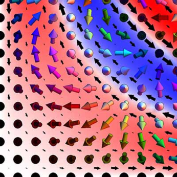
Figure 4: Neutral stripe configuration satisfying non-trivial corner boundary conditions. Red (blue) background indicates positive (negative) skyrmion density $q$, black 2D arrows the superfluid velocity $\mathbf{v}$, and shaded 3D arrows the magnetization $\hat{n}$.

For completeness, we first briefly consider $f(z)$ given by higher order polynomials. The corresponding stripe solutions are not doubly periodic, but satisfy non-trivial boundary conditions. For example, we show the magnetization $\hat{n}$, skyrmion density $q$, and superfluid velocity $\mathbf{v}$ for $f(z)=iz^{2}$ in Fig. 4. This solution satisfies corner boundary conditions with zero normal component to both the superfluid velocity $\mathbf{v}$ and spin current $\mathbf{J}^{i}_{\mu}=\hat{n}^{i}\mathbf{v}_{\mu}-\epsilon^{ijk}\hat{n}^{j}\nabla_{\mu}\hat{n}^{k}/2$.

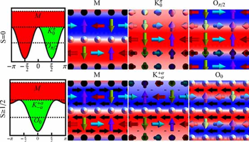
Figure 5: Stripe configurations for different boundary conditions in $S\geq 1/2$ spinor condensate (bottom row) and $S=0$ ordinary ferromagnets (top row). Red (blue) background indicates positive (negative) skyrmion density $q$, black 2D arrows the superfluid velocity $\mathbf{v}$, and shaded 3D arrows the magnetization $\hat{n}$. Notice $\hat{n}_{x}$, $\hat{n}_{y}$ $(\hat{n}_{z})$ wind horizontally (oscillate vertically). The first column shows schematic plots of the classical periodic potential $U(\alpha)$ controlling the evolution of the angular variable $\alpha$ for $\hat{n}_{z}=\cos(\alpha)$. Labels for the corresonding type of solution are below the dashed lines indicating the corresponding constant of motion $E$. For $E$ above the maximum of $U$, $\alpha(u)$ is montonic in the coordinate $u$ giving rise to periodic stripe configurations labeled $M$ with $\hat{n}_{z}$ covering the entire range $\pm 1$. For $E$ at a potential maximum, kink solutions connecting the maxima $\alpha_{1}$, $\alpha_{2}$ give rise to single domain wall configurations in $\hat{n}_{z}$ labeled $K_{\alpha_{1}}^{\alpha_{2}}$. For a given value of $C$, kink solutions occur at one specific value of $E$. For $E$ below the maximum, $\alpha$ oscillates about a minimum located at $\alpha_{0}$ giving rise to periodic stripe configuration with $\hat{n}_{z}$ oscillating about $\cos(\alpha_{0})$. Notice that monotonic solutions $M$ are qualitatively similar for both $S\geq 1/2$ spinor condensate and $S=0$ ordinary ferromagnets. In contrast, spinor condensate (ordinary) ferromagnets have a single (two distinct) $2\pi$ ($\pi$) kink solutions $K$ centered about $\alpha=0$ ($\alpha=\pm\pi/2$). In addition, there is a single (two distinct) oscillatory solutions $O$ also centered about $\alpha=0$ ($\alpha=\pm\pi/2$) for spinor condensate (ordinary) ferromagnets.

From here on, we focus on $f(z)=iz$ with the corresponding solutions doubly periodic and describing stripe configurations. The different types of behavior for $\alpha(u)$ are illustrated schematically along with the resulting configurations for $\hat{n}$ in Fig. 5. $E$ above the global maximum corresponds to $\alpha(u)$ monotonic in $u$ which from here on we denote as $M$. This solution describes a periodic stripe solution with $\hat{n}_{z}$ varying over the entire range $\pm 1$. $E$ at a local maximum corresponds to a kink solution for $\alpha(u)$ connecting $\alpha_{1}$ to $\alpha_{2}$ denoted as $K_{\alpha_{1}}^{\alpha_{2}}$. This solution describes a single domain wall configuration in $\hat{n}_{z}$ and is the analog of the localized solution described earlier. $E$ below a local maximum corresponds to $\alpha(u)$ oscillating near a fixed value $\alpha_{0}$ denoted as $O_{\alpha_{0}}$. Finally, $E$ below the global minimum is forbidden, denoted as $F$.

Notice that for $S=0$, $S=1/2$, $S>1/2$, the $\cos(2\alpha)$ term in the potential $U(\alpha)$ of Eq. 17 is negative, zero, and positive. For the montonic solutions $M$, this does not affect the qualitative behavior of the resulting periodic stripe configurations. For kink solutions $K$ connecting $0\rightarrow 2\pi$ or $-\pi\rightarrow+\pi$ ($0\rightarrow\pi$ or $-\pi\rightarrow 0$), the resulting single domain wall carrys zero net skyrmion charge (positive or negative skyrmion charge) for spinor condensate (ordinary) ferromagnets. Oscillatory solutions $O$ also have different behavior with oscillations centered about $\hat{n}_{z}\approx\pm 1$ ($\hat{n}_{z}\approx 0$) for spinor condensate (ordinary) ferromagnets.

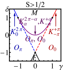
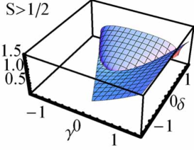
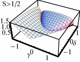
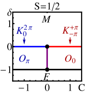
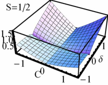
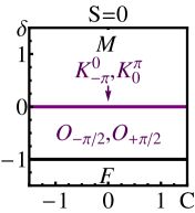
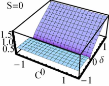
Figure 6: Classification of solutions (2D plots) and total energy density (3D plots) for stripe configurations given different boundary conditions in $S>1/2$ (top row) and $S=1/2$ (bottom left) spinor condensate as well as $S=0$ (bottom right) ordinary ferromagnets. Fig. 5 illustrates the corresponding configurations. $\gamma$ controls a constant contribution to the superfluid velocity. $\delta$ controls the energy of an associated classical mechanics problem giving the evolution of $\hat{n}_{z}=\cos(\alpha)$, the $\hat{z}$ component of the magnetization. Monotonic solutions $M$ have $\hat{n}_{z}$ covering the entire range $\pm 1$. Kink solutions $K_{\alpha_{1}}^{\alpha_{2}}$ describe single domain wall configurations with $\hat{n}_{z}$ connecting $\cos(\alpha_{1})$ to $\cos(\alpha_{2})$. Oscillatory solutions $O_{\alpha_{0}}$ have $\hat{n}_{z}$ oscillating about $\cos(\alpha_{0})$. Notice kink solutions $K$ always separate monotonic $M$ from oscillatory $O$ solutions. For $S>1/2$ spinor condensate ferromagnets, notice the two distinct oscillatory and kink solutions for each $\gamma$, $\delta$ in the region near the origin which are absent for $S=1/2$. For $S=0$ ordinary ferromagnets, there is no dependence on $C$.

For ordinary ferromagnet with $S=0$, we parametrize $E=k^{2}(1+2\delta)/4$ and find the solution of Eq. 16 and the total energy of Eq. 18 given by

$$\alpha(u) =\pi/2\pm\text{am}\left(ku\sqrt{1+\delta},(1+\delta)^{-1}\right)$$

$$\bar{\mathcal{H}} =\frac{Sk^{2}}{2}\left[-\frac{\delta}{2}+\theta(1+\delta)\right]$$ (24)

where $\bar{\mathcal{H}}$ is the total energy density given by the averaging $\mathcal{H}$ over the unit cell. Also, $\text{am}(x,m)$ is the Jacobi amplitude function and we define

$$\theta(m)=m\frac{\text{Re}[E(m^{-1})]}{\text{Re}[K(m^{-1})]}$$ (25)

with $K$ ($E$) the complete elliptic integral of the first (second) kind. For $\delta<-1$ the solution is forbidden $F$. For $-1\leq\delta<0$ there are two oscillatory solutions at the $\pm\pi/2$ minima $O_{\pm\pi/2}$. For $\delta=0$ there are two kink solutions $K_{0}^{+\pi}$ and $K_{-\pi}^{0}$. For $\delta>0$ the solution is monotonic $M$. We show the classification of solutions along with the total energy density for ordinary ferromagnets in the bottom left of Fig. 6. Notice the solutions and total energy density do not depend on $C$. This is because $C$ enters through the superfluid velocity which is absent from the Lagrangian for ordinary ferromagnets.

For spinor condensate ferromagnets with $S=1/2$, we parameterize the constant of motion $E=|C|k^{2}(1+2\delta)$ and find the solution of Eq. 16 and the total energy density from Eq. 18 given by

$$\alpha(u) =\cos^{-1}(C/|C|)+2\text{am}\left(ku\sqrt{|C|(1+\delta)},(1+\delta)^{-1}\right)$$

$$\bar{\mathcal{H}} =k^{2}\left[\frac{(|C|-1)^{2}}{8}-\frac{\delta|C|}{2}+|C|\theta(1+\delta)\right]$$ (26)

depends only on $|C|$. For $\delta<-1$ the solution is forbidden $F$. For $-1\leq\delta<0$ there is one oscillatory solution $O_{\pi}$ ($O_{0}$) for $C<0$ ($C>0$). For $\delta=0$ there is one kink solution $K_{0}^{2\pi}$ ($K_{-\pi}^{+\pi}$) for $C<0$ ($C>0$). For $\delta>0$ the solution is monotonic $M$. We show the classification of solutions along with the total energy density for $S=1/2$ spinor condensate ferromagnets in the bottom right of Fig. 6.

For spinor condensate ferromagnets with $S>1/2$ we parameterize the constant of motion $E=(2S-1)k^{2}(1+2\delta)/4$ and the constant $C=(2S-1)\gamma/2S$. With $\gamma=\tau$ and $\delta=-1+2\sigma\tau$ where $\sigma=\pm 1$ we find one solution for Eq. 16 while the total energy density from Eq. 18 given by

$$\alpha(u) =\text{Arg}\left[-\frac{\tau-\sigma+2\sqrt{\tau(\tau-\sigma)}s(u)+\tau s(u)^{2}}{1+\sigma\tau-\sigma\tau s(u)^{2}}\right]$$

$$\bar{\mathcal{H}} =\frac{Sk^{2}}{2}\left[h_{0}+(2S-1)j_{0}\right]$$ (27)

where we define the auxiliary function

$$s(u) =\sin(ku\sqrt{(1-\sigma\tau)(2S-1)})$$ (28)

in the solution for $\alpha(u)$ and the functions

$$h_{0} =\frac{((2S-1)\tau-\sigma S)^{2}}{4S}$$

$$j_{0} =\begin{cases}\sigma\tau\sqrt{\tau-\sigma}&0\leq\sigma\tau\leq 1\\ 0&\text{otherwise}\end{cases}$$ (29)

for the total energy density. With $\gamma=r\sinh(\tau)$ and $\delta=-1+2r\sinh(\tau)$ we find two solutions for Eq. 16 and the total energy density from Eq. 18 given by

$$\alpha_{\pm}(u)= \text{Arg}\left[-\frac{\cosh(\tau/4)e^{\pm iw(u)}\mp\sinh(\tau/4)}{\sinh(\tau/4)e^{\pm iw(u)}\mp\cosh(\tau/4)}\right]$$

$$\bar{\mathcal{H}}= \frac{Sk^{2}}{2}\left[h+(2S-1)j\mp(2S-1)k\right]$$ (30)

where we define the auxiliary function

$$w(u)= \text{am}\left[ku\sqrt{2r(2S-1)},\frac{1+r-r\cosh(t)}{2r}\right]$$ (31)

in the solutions for $\alpha(u)$ and the functions

$$h= \frac{1-(2S-1)\delta}{2}+\frac{(2S-1)^{2}\beta^{2}}{4S}$$

$$j= \frac{\text{Re}[2\sqrt{r}E(\omega)]}{\text{Re}[K(\omega)/\sqrt{r}]}+$$

$$\frac{\text{Re}[2\sqrt{r}[\cosh(t/2)^{2}\Pi(-\sinh(t/2)^{2},\omega)-K(\omega)]]}{\text{Re}[K(\omega)/\sqrt{r}]}$$

$$k= \begin{cases}\frac{\text{Re}[\pi r\sinh(t)]}{\text{Re}[K(\omega)\sqrt{2/r}]},&O_{\pi},O_{0}\ \text{phase}\\ 0&\text{otherwise}\end{cases}$$

$$\omega= \frac{1+r-r\cosh(\tau)}{2r}$$ (32)

for the total energy density where $\Pi(m,n)$ is the complete elliptic integral of the third kind. We show the classification of solutions along with the total energy density for $S>1/2$ spinor condensate ferromagnets in the top row of Fig. 6. The boundaries between solutions of different types are given by $\delta=-1+2\beta$, $\delta=-1-2\beta$, $\delta=\beta^{2}$. For increasing $\gamma$, notice kink solutions evolve from just one $K_{0}^{2\pi}$ through a region with two $K_{\alpha}^{2\pi-\alpha}$ and $K_{-\alpha}^{+\alpha}$, to just one $K_{-\pi}^{+\pi}$ for $\gamma<-1$, $-1<\gamma<+1$, $+1<\gamma$, respectively. The kink solutions separate the monotonic solutions $M$ from the oscillatory solutions. For increasing $\gamma$, the oscillatory solutions also evolve from just one $O_{\pi}$ to a region with two $O_{\pi}$ and $O_{0}$, to just one $O_{0}$ for $\delta<-1-2\gamma$, $-1+2\gamma\geq\delta\geq-1-2\gamma$, $\delta<-1+2\gamma$, respectively.

VI Discussion

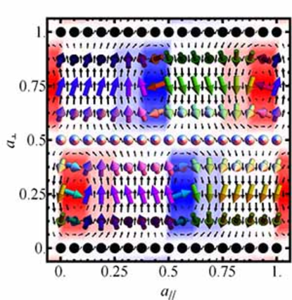
Figure 7: Numerically optimized configuration for two-dimensional spinor condensate ferromagnets with an effective dipolar interaction modified by rapid Larmor precession. The magnetic field $\hat{B}=\hat{x}$ inducing Larmor precession lies along the horizontal axis in the plane. Lattice constants are $a_{\parallel}=90$ $\mu$m and $a_{\perp}=42$ $\mu$m. Red (blue) background indicates positive (negative) skyrmion density $q$, black 2D arrows the superfluid velocity $\mathbf{v}$, and shaded 3D arrows the magnetization $\hat{n}$.

Having presented a unified description of both localized and extended stripe solutions in ordinary and spinor condensate ferromagnets, we now turn to how these solutions offer insight into different physical phenomena. We first consider quantum Hall systems. As discussed in Sec. III, configurations for quantum Hall ferromagnets away from quantum Hall plateaus carry net skymrion charge Lee and Kane (1990); Sondhi et al. (1993); Lejnell et al. (1999); Fertig et al. (1994); Timm et al. (1998). Thus, solutions for the ordinary ferromagnet describing collections of localized skyrmions carrying net charge as shown in the left of Figs. 1 and 2 have been used extensively in this regime.

However, we showed in Sec. V that these solutions of localized topological objects can be derived in a unified framework along with extended stripe solutions. There have been a number of studies on the possibility of quantum Hall states with stripe order. At high Landau levels and with frozen spin degrees of freedom, Coloumb interaction may directly favor charge density waves as predicted theoretically Koulakov et al. (1996); Moessner and Chalker (1996) and verified experimentally Lilly et al. (1999); Du et al. (1999). Such states are not directly comparable to the stripe solutions we describe which have fixed total density and stripe order in the relative density. However, stripe order has also been proposed Demler et al. (2002); Côté et al. (2002); Brey and Fertig (2000) and experimental evidence observed Gusev et al. (2007) in the context of quantum Hall bilayers. Here, even though the total density between layers is fixed, both interlayer coherence and relative density imbalance can develop. The isospin degree of freedom that arises can be used to define an appropriate magnetization vector $\hat{n}$. Here, the phase of the interlayer coherence gives the orientation of $\hat{n}_{x}$, $\hat{n}_{y}$, while the relative density imbalance gives $\hat{n}_{z}$. States with skyrmion stripe order and winding $\hat{n}_{x}$, $\hat{n}_{y}$ have been proposed that are direct analogs of the configurations shown in the top row of Fig. 5.

For spinor condensate ferromagnets, experiments at Berkeley suggest the possibility of a condensate with crystalline magnetic order Vengalattore et al. (2008, 2009). This crystalline order arises from an effective dipolar interactions modified by rapid Larmor precession and reduced dimensionality. It can drive dynamical instabilities of the uniform state which occur in a characteristic pattern Cherng and Demler (2009); Kawaguchi et al. (2009). Modes controlling the component $\hat{n}$ parallel (perpendicular) to the magnetic field in spin space are unstable along wavevectors perpendicular (parallel) to the magnetic field in real space. Instabilities of this type can give rise to the spin textures shown in the stripe solutions of the bottom row in Fig. 5. Here, $\hat{n}_{z}$ is modulated along the $y$ direction while $\hat{n}_{x}$, $\hat{n}_{y}$ wind along the $x$ direction.

In the companion paper Levitov et al. (2010), we have performed a systematic numerical study of minimal energy configurations for spinor condensate ferromagnets with dipolar interactions. This is made possible by the use of symmetry operations combining real space and spin space operations to distinguish different symmetry classes of solutions. For applied magnetic field in the plane $\hat{B}=\hat{x}$ corresponding to current experiments, we show the lowest energy configuration in Fig. 7.

Notice $\hat{n}_{z}$ is modulated between $\pm 1$ just as in the monotonic $M$ solutions shown in Fig. 5. In addition, the $\hat{n}_{x}$, $\hat{n}_{y}$ components wind along the horizontal axis. However, notice the winding in the $\hat{n}_{x}$, $\hat{n}_{y}$ components is not uniform as in the solutions we find in this paper. In addition, the winding changes from clockwise to counter-clockwise halfway along the horizontal axis. For the solutions we find in this paper, the skyrmion density forms stripes of opposite charge parallel to the horizontal axis. For the lowest energy configuration in Fig. 7, the non-uniform winding leads to concentration of the skyrmion density in smaller regions and modulation in the sign of the skyrmion density along the $x$ axis. We find minimal energy configurations in other symmetry classes are generally of this type with $\hat{n}_{z}$ oscillating between $\pm 1$ along $y$ and $\hat{n}_{x}$, $\hat{n}_{y}$ winding along $x$. However, the detailed form of the winding along $x$ varies for different classes.

Thus we see that the exact solutions for spinor condensate ferromagnets without dipolar interactions provides a more transparent physical picture for the numerical solutions with dipolar interactions. This can be seen as follows. The solutions we find in this paper describe overall neutral collections of skyrmion and anti-skyrmion topological objects. The neutrality constraint comes from the long-ranged divergence of the skyrmion interaction and remains even when considering additional spin interactions such as the dipolar interaction. Morever, skyrmions and anti-skyrmions themselves have a non-trivial spin texture which is evident in Fig. 5 showing the solutions of this paper. When dipolar interactions are included, such spin textures can take advantage of the gain in dipolar interaction energy without chaning their qualitative structure. However, quantitative details for minimal energy configurations such as the one shown in Fig. 7 require detailed analysis of the competition between dipolar interactions, skyrmion interactions, and spin stiffness.

In conclusion, we have presented the low-energy effective theory of spinor condensate ferromagnets. This effective theory describes the superfluid velocity and magnetization degrees of freedom and can be written as a non-linear sigma model with long-ranged interactions between skyrmions, the topological objects of the theory. Quantum Hall ferromagnets share a similar effective theory with long-ranged skyrmion interactions. For the case of spinor condensate ferromagnets, we find exact solutions for the non-linear equations of motion describing neutral configurations of skyrmions and anti- skyrmions carrying zero net skyrmion charge. These solutions describe within a unified framework both collections of localized topological objects as well as extended stripe configurations. In particular, they can be used to understand aspects of non-trivial spin textures in both quantum Hall ferromagnets as well as spinor condensate ferromagnets with dipolar interactions.