Egalitarian Improvement to Democracy: Quark renormalization constants in $N_{f}=2$ QCD

Abstract:

We present our results on the non-perturbative evaluation of the renormalization constant for the quark field, $Z_{q}$, in Landau gauge within RI-MOM scheme. Using three lattice spacing we are able to isolate lattice artefacts of various origin, both perturbative and non-perturbative. In particular, the existence of the dimension-two gluon-condensate is discussed, and confirmed.

1 Introduction

As any other way of computing matrix elements, lattice QCD requires calculation of the renormalisation constants, which relate bare quantities to the physical ones. In our particular case the renormalization constants will be dependent not only on the scale, but also on the lattice parameters, such as light quark mass and lattice spacing. This dependence turns out to be remarkably strong in case of the latter. Even if the lattice computation contains only $O(a^{2})$ lattice artefacts, the bare quantities differ from the continuum ones by $O(g^{2})\simeq O(1/\log(a^{2}))$ which is unacceptable. Renormalization restores the $O(a^{2})$ accuracy. While some perturbative methods to calculate the constants exist, it is obviously preferable to do it in a consistent manner, i.e. non-perturbatively. Although in some cases the results may be similar, there is no guarantee for the validity of the perturbative calculation.

Our method of preference is the so-called RI’MOM scheme. It involves the computation of Green functions of quarks, gluons, ghosts, at large enough momenta in a fixed gauge, usually the Landau gauge. This gives the renormalisation constant $Z(\mu)$ at many values of the scale $\mu$. We have to note here, that even though we advocate the completely non-perturbative approach, the conversion to other renormalization schemes has to fall back onto perturbative methods. Here we use perturbative QCD to convert MOM into $\overline{\rm MS}$ and run to 2 GeV. The running of $Z_{\mathrm{M}OM}(\mu)$ is a very powerful testing tool: perturbative QCD is only useful if we are in the perturbative regime, i.e. at large enough momenta. The only way to check if this is the case is to compare lattice data with the perturbative running. It turns out that this is not always so.

To calculate the renormalization constants we must fix the gauge, and we perform all calculation in the Landau gauge. Wilson operator expansion suggests the presence of the non-vanishing vacuum expectation value of the only dimension-two operator in the Landau gauge: $A^{2}\equiv A^{a}_{\mu}A^{a\mu}$, and that it is not small [1, 2],[3]. This contribution to the OPE will scale as $1/p^{2}$ up to logarithmic corrections. To argue that this is a continuum feature we must check that the $1/p^{2}$ term scales well with the lattice spacing when expressed in physical units.

In general, our museum of artefacts has a number of exhibitions. The $O(a^{2})$ artefacts can be quite large since we consider large momenta, while finite volume artefacts are minor. There are two main types of $O(a^{2})$ artefacts: $O(a^{2}p^{2})$ artefacts which respect the continuum $O(4)$ rotation symmetry, and the ones which do not. The latter appear due to the explicit breaking of the rotational symmetry, which, on the lattice, is reduced to the hypercubic symmetry $H_{4}$. After removing these, we will identify the $O(a^{2}p^{2})$ artefacts non-perturbatively by doing a fit of the running $Z(\mu)$ which will include the perturbative running, the condensate and a term proportional to $a^{2}p^{2}$.

For the elimination of hypercubic artefacts several methods have been proposed in literature: the democratic one, the perturbative correction and the non-perturbative “egalitarian” one. The perturbative one deserves a separate paper, so we will focus on two others. We will demonstrate to what extent the “half-fishbone” structure, which raw lattice results for $Z_{q}$ always exhibit and which is a dramatic illustration of hypercubic artefacts, is corrected by every method.

Although the issues raised here concern all the renormalisation constants as well as the QCD coupling constant, we will concentrate in the following on $Z_{q}$, that renormalizes the quark field

$$q_{R}=Z_{q}^{1/2}q_{B}$$ (1)

where $q_{B}$ ($q_{R}$) is the bare (renormalized) quark field.

2 Simulation details

For the details about twisted mass and tree-level improved Symanzik gauge actions please refer to refs. [6, 7, 8, 9]. Here we will just briefly mention the essential parts for our presentation (See Tab. 1).

The Wilson twisted mass fermionic lattice action for two flavours of mass degenerate quarks reads (in the so called twisted basis [4, 10] )

$$\begin{split}S_{\mathrm{tm}}^{\rm F}=&\,a^{4}\sum_{x}\Bigl{\{}\bar{\chi}_{x}\left[D_{\rm W}+m_{0}+i\gamma_{5}\tau_{3}\mu_{q}\right]\chi_{x}\Bigr{\}}\,,\\ &D_{\rm W}=\frac{1}{2}\gamma_{\mu}\left(\nabla_{\mu}+\nabla_{\mu}^{*}\right)-\frac{ar}{2}\nabla_{\mu}\nabla_{\mu}^{*}\,,\end{split}$$ (2)

where $m_{0}$ is the bare untwisted quark mass and $\mu_{q}$ the bare twisted quark mass, $\tau_{3}$ is the third Pauli matrix acting in flavour space and $r$ is the Wilson parameter, which, as usually, is set to $r=1$ in the simulations. The twisted Dirac operator is defined as

$$D_{\rm tw}\equiv D_{\rm W}+m_{0}+i\gamma_{5}\tau_{3}\mu_{q}$$ (3)

The bare quark mass $m_{0}$ is related as usual to the so-called hopping parameter $\kappa$, by $\kappa=1/(8+2am_{0})$. Twisted mass fermions are said to be at maximal twist if the bare untwisted mass is tuned to its critical value, $m_{\mathrm{crit}}$. This corresponds to setting the so-called untwisted PCAC mass to zero, so it requires additional tuning during the simulation.

In the gauge sector the tree-level Symanzik improved gauge action (tlSym) [5] is used:

$$S_{g}=\frac{\beta}{3}\sum_{x}\Biggl{(}b_{0}\sum_{\begin{subarray}{c}\mu,\nu=1\\ 1\leq\mu<\nu\end{subarray}}^{4}\{1-\mathbb{R}\text{e}\text{Tr}(U^{1\times 1}_{x,\mu,\nu})\}\Bigr{.}\Bigl{.}+b_{1}\sum_{\begin{subarray}{c}\mu,\nu=1\\ \mu\neq\nu\end{subarray}}^{4}\{1-\mathbb{R}\text{e}\text{Tr}(U^{1\times 2}_{x,\mu,\nu})\}\Biggr{)}\,,$$ (4)

where $\beta\equiv 6/g_{0}^{2}$, $g_{0}$ being the bare lattice coupling and we set $b_{1}=-1/12$ (with $b_{0}=1-8b_{1}$ as dictated by the requirement of continuum limit normalization). The overview of the ensembles used for this work can be found in Tab. 1. From our previous simulations we deduced that fortunately $Z_{q}$ does not depend within uncertainties on the sea-quarks mass and on the lattice volume. So here we keep both quark mass and volume fixed.

$\beta$	$a\mu_{q}$	Volume	# confs dim 3	# confs dim 4.
$3.9$	0.004 0.0064 0.010	$24^{3}\times 48$	$120$ $20$ $20$	$100$ $20$ $20$
$4.05$	0.006 0.003 0.006 0.008 0.012	$24^{3}\times 48$ $32^{3}\times 64$ $32^{3}\times 64$ $32^{3}\times 64$ $32^{3}\times 64$	$100$ $20$ $20$ $20$ $20$	$100$ - - - -
$4.2$	0.0065 0.002	$32^{3}\times 64$ $24^{3}\times 48$	$100$ -	$100$ $100$

Table 1: ETMC ensembles used for this work, “dim 3” refers to the local operators (V, A, S, P) while “dim 4” refer to the operators with one derivative (O44, O14, etc).

To compute the renormalization constants for the quark propagator we need to fix the gauge and calculate the 2-point quark Green functions on each configuration. We do this using a local source taken at a random point on the lattice which reduces the correlation between successive configurations:

$$S(y,x_{0})^{a,\alpha;b_{0},\beta_{0}}_{i}=D_{\rm tw}^{-1}(y,x)^{a,\alpha;b,\beta}so^{b,\beta}(x)\qquad so^{b,\beta}_{i}(x)=\delta_{x,x_{0}}\delta_{b,b_{0}}\delta_{\beta,\beta_{0}}$$ (5)

where $i=u,d$ labels isospin. Thereafter we perform the Fourier transform of the incoming quark which is a $12\times 12$ complex matrix

$$S_{i}(p)\equiv\sum_{y}e^{-ip(y-x_{0})}\,S_{i}(y,x_{0})$$ (6)

and the outgoing quark

$$S^{\dagger 5}_{i}(p)=\gamma_{5}S^{\dagger}_{\bar{i}}(p)\gamma_{5}$$ (7)

where $\bar{u}\equiv d;\bar{d}\equiv u$. We define the quark renormalization constant $Z_{q}$ as

$$Z_{q}(p)\equiv\frac{1}{12\,p^{2}}\;<{\rm Tr}[S^{-1}(p)p\!\!\!/]>$$ (8)

where $<...>$ means here the average over the chosen ensemble of thermalized configurations.

3 Artefacts

3.1 Hypercubic $H(4)$-extrapolation

A first kind of artefacts that can be systematically cured [11, 12] are those arising from the breaking of the rotational symmetry of the Euclidean space-time when using an hypercubic lattice, where this symmetry is restricted to the discrete $H(4)$ isometry group. It is convenient to compute first the average of any dimensionless lattice quantity $Q(ap_{\mu})$ over every orbit of the group $H(4)$. In general several orbits of $H(4)$ correspond to one value of $p^{2}$. Defining the $H(4)$ invariants

$$p^{[4]}=\sum_{\mu=1}^{4}p_{\mu}^{4}\qquad p^{[6]}=\sum_{\mu=1}^{6}p_{\mu}^{6}$$ (9)

it happens that the orbits of $H(4)$ are labeled by the set $p^{2},a^{2}p^{[4]},a^{4}p^{[6]}$. Group theory tells us that any $H(4)$-invariant polynome will only depend on the four invariants $p^{[2i]}$ with $i=1,2,3,4$ [11, 12]. As a consequence of the upper cut for momenta, the first three of these invariants suffice to label all the orbits we deal with and hence any presumed dependence on $p^{[8]}$ is neglected. We have to admit that our action is obviously non-polynomial, but perturbative results suggest that up to a certain order the renormalization constant will be such, so it is sensible to assume this feature. Later we will be able to check that it leads to consistent results, proving our assumption. Moreover, in the continuum limit the effect of $a^{2}p^{[4]},a^{4}p^{[6]}$ vanishes. We can thus define the quantity $Q(ap_{\mu})$ averaged over $H(4)$ as

$$Q(a^{2}\,p^{2},a^{4}p^{[4]},a^{6}p^{[6]},a^{2}\Lambda_{\rm QCD}^{2}).$$ (10)

If the lattice spacing is small enough such that $\epsilon=a^{2}p^{[4]}/p^{2}\ll 1$, the dimensionless lattice correlation function defined in Eq. (10) can be expanded in powers of $\epsilon$ and truncated:

$$Q(a^{2}\,{p}^{2},a^{4}p^{[4]},a^{6}p^{[6]},a^{2}\Lambda_{\rm QCD}^{2})=Q(a^{2}p^{2},a^{2}\Lambda_{\rm QCD}^{2})+\left.\frac{dQ}{d\epsilon}\right|_{\epsilon=0}a^{2}\frac{p^{[4]}}{p^{2}}+\cdots$$ (11)

The basic method is to fit from the whole set of orbits, sharing the same $p^{2}$, the coefficient $dQ/d\epsilon$ and get the extrapolated value of $Q$, free from $H(4)$ artefacts. The fit is performed in a momentum window between $(p-\delta,p+\delta)$ to extract the extrapolated value of $Q$ for the momenta $p$ in the window, and then we shift to the next window etc.

Such method, which we call SWF, “sliding window fit”, is quite reliable since the extrapolation does not rely on any particular assumption for the coefficients of the Taylor expansion. We can then estimate the systematic error by varying the width of the fitting window. If we further assume that the coefficient

$$\left.R(a^{2}p^{2},a^{2}\Lambda_{\rm QCD}^{2})=\frac{dQ\left(a^{2}p^{2},0,0,a^{2}\Lambda_{\rm QCD}^{2}\right)}{d\epsilon}\right|_{\epsilon=0}$$ (12)

has a smooth dependence on $a^{2}p^{2}$ over a given momentum window, we can expand $R$ as

$$R=c_{a2p4}+c_{a4p4}a^{2}p^{2}$$ (13)

and make a global fit over a wide range of momenta:

$$Q(a^{2}\,{p}^{2},a^{4}p^{[4]},a^{6}p^{[6]},a^{2}\Lambda_{\rm QCD}^{2})=Q(a^{2}p^{2},a^{2}\Lambda_{\rm QCD}^{2})+c_{a2p4}a^{2}\frac{p^{[4]}}{p^{2}}+c_{a4p4}a^{4}p^{[4]}+\cdots$$ (14)

We will refer to this method as OWF, “one window fit”.

4 Lattice results and Hypercubic corrections

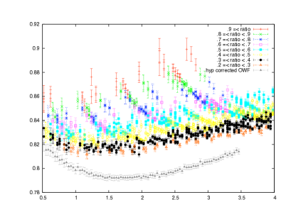
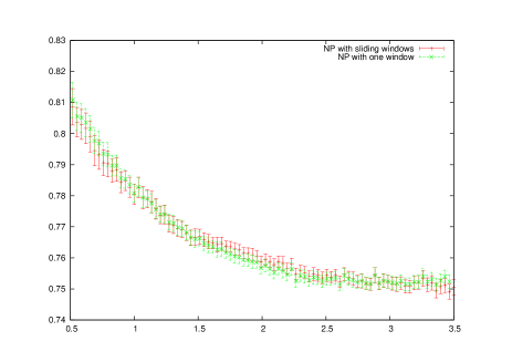
Figure 1: On the l.h.s. we show the raw data for $\beta=3.9$, $Z_{q}^{\mathrm{latt}}(a^{2}\,p^{2},a^{4}p^{[4]},a^{6}p^{[6]},ap_{4},a^{2}\Lambda_{\rm QCD}^{2})$. The “half-fishbone structure” due to hypercubic artefacts is clearly seen. There is one point for every cubic (3-D) orbit. On the r.h.s we show, using the OWF, the non-perturbatively corrected data. As on l.h.s., there is one point for every cubic (3-D) orbit.

The hypercubic artefacts are clearly visible on the raw lattice data for $Z_{q}^{\mathrm{latt}}$ as the so-called “half-fishbone” structure [13] shown in fig 1. The color code shows the value of the ratio $p^{[4]}/(p^{2})^{2}$ which is between 0.25 and 1. The values which are closer to one are “least democratic” or “tyrannic” ones. We see, as expected, that the tyrannic points are more affected by the artefact. We also see that the gap between $Z_{q}^{\mathrm{latt}}(a^{2}\,p^{2},a^{4}p^{[4]},a^{6}p^{[6]},ap_{4},a^{2}\Lambda_{\rm QCD}^{2})$ at a given $q^{2}$ can be as large as 0.07, i.e. about 10%. Taking a naive average without a correct treatment of this artefact would leave a systematic upward shift of about 5 %.

The oldest method to alleviate this problem is the “democratic selection”. It amounts to keeping only, say, the violet points in Fig. 1, or, in case of low statistics, being less restrictive, the violet and yellow ones. It works to a certain extent, but obviously we still have an upward shift compared to H4-method, which is not negligible.

While performing systematic treatment using H4-method, we only expand up to $p^{[4]}$ since the higher order terms turn out to be negligible. In the l.h.s of Fig. 1, we show the comparison of hypercubic corrected data after applying OWF and SWF for the case $\beta=3.9$ . The difference does not appear to be large which is rather encouraging. The OWF gives a slightly smoother result.

$\beta$	$a^{2}$ fm2	$c_{a2p4}$	$c_{a4p4}$	$c_{a2p4}/g^{2}$	$c_{a4p4}/g^{2}$	$\chi^{2}$/d.o.f
$3.9$	0.00689	0.067(4)	-0.0149(10)	0.044(3)	-0.0097(7)	4.1
$4.05$	0.00456	0.065(3)	-0.0144(5)	0.044(2)	-0.0097(3)	0.53
$4.2$	0.00303	0.055(11)	-0.0124(4)	0.039(8)	-0.0089(3)	0.98

Table 2: Results for the slope in $a^{2}\,p^{[4]}/p^{2}$ and $a^{4}\,p^{[4]}$ and the same divided by $g^{2}$ in the one window fits.

The fitted values of $c_{a2p4}$ and $c_{a4p4}$ from the one window fit are given in Tab. 2 as well as the same divided by $g^{2}$, since perturbation theory expects at least for $c_{a2p4}$ to be $\propto g^{2}$. Before dividing by $g^{2}$ a small scaling violation is apparent, and much less so afterwards. The $\chi^{2}$ in Tab. 2 is not good for $\beta=3.9$, apparently due to some structure at the lower end of the plot, but remember it uses only two hypercubic parameters. Of course, this point is further away from the continuum than both other points.

5 Results and Conclusion

Once the hypercubic corrections are performed we make a fit for every $\beta$ according to the following formula

$$Z_{q}^{\mathrm{NPsubtracted}}(a^{2}p^{2}) = Z_{0}\,c_{0Z_{q}}(q^{2},\mu^{2})\left(1+\frac{c_{1overp2}}{p^{2}}\right)+c_{a2p2}\;a^{2}\,p^{2}$$ (15)

where $c_{0Z_{q}}(q^{2},\mu^{2})$ is the perturbative running of $Z_{q}$ [14], $c_{a2p2}$ is a hypercubic insensitive lattice artefact, and $c_{1overp2}$ is due to the $g^{2}\langle A^{2}\rangle$ condensate. Combining several analysis methods we get

$$g^{2}(\mu^{2})\langle A^{2}\rangle_{\mu^{2}} = 2.25(40)\left({}^{+0.75}_{-1.0}\right)\;\mathrm{GeV}^{2}\quad\mu=10\,\mathrm{GeV}$$

$$Z_{q}^{\mathrm{pert}}((10\,{\mathrm{GeV}})^{2},g^{2}_{\mathrm{bare}}) = 0.741(3)(7)-0.305(25)\,(g^{2}_{\mathrm{bare}}-1.5)$$

$$Z_{q}^{\mathrm{pert}}((2\,{\mathrm{GeV}})^{2},g^{2}_{\mathrm{bare}}) = 0.773(3)(7)-0.319(20)\,(g^{2}_{\mathrm{bare}}-1.5)$$

To conclude, we calculated $Z_{q}$ from the ETMC gauge configurations in the RI-MOM scheme. We demonstrated effectiveness of the H4-method of removing hypercubic artefacts. From the resulting hypercubic corrected function $Z_{q}(a^{2}p^{2},a^{2}\Lambda_{\rm QCD}^{2})$ we perform a fit to an Ansatz consisting of the perturbative running, a non perturbative $1/p^{2}$ term and rotationally-symmetric lattice spacing artefact proportional to $a^{2}p^{2}$. The fits are good and $a^{2}p^{2}$ term scales almost perfectly in lattice units, as expected. The $g^{2}\langle A^{2}\rangle$ term scales rather well in physical units as expected, though less accurate. Therefore we advocate the presence of the non-perturbative condensate in the quark renormalization constant. More detailed analysis and even more rigorous proof will be presented in a separate paper soon.

References

- [1] Ph. Boucaud et al., JHEP 0601 (2006) 037 [arXiv:hep-lat/0507005];
- [2] B. Blossier, Ph. Boucaud, F. De Soto, V. Morenas, M. Gravina, O. Pene and J. Rodriguez-Quintero [ETM Collaboration], arXiv:1005.5290 [hep-lat].
- [3] K. G. Chetyrkin and A. Maier, arXiv:0911.0594 [hep-ph].
- [4] R. Frezzotti, P. A. Grassi, S. Sint and P. Weisz [Alpha collaboration], JHEP 0108 (2001) 058 [arXiv:hep-lat/0101001].
- [5] P. Weisz, Nucl. Phys. B 212 (1983) 1.
- [6] Ph. Boucaud et al. [ETM Collaboration], Phys. Lett. B 650 (2007) 304 [arXiv:hep-lat/0701012].
- [7] Ph. Boucaud et al. [ETM collaboration], Comput. Phys. Commun. 179 (2008) 695 [arXiv:0803.0224 [hep-lat]].
- [8] C. Urbach [ETM Coll.], PoS LAT2007 (2007) 022 [0710.1517 [hep-lat]].
- [9] P. Dimopoulos et al. [ETM Collaboration], arXiv:0810.2873 [hep-lat].
- [10] R. Frezzotti and G. C. Rossi, JHEP 0408 (2004) 007 [arXiv:hep-lat/0306014].
- [11] D. Becirevic, P. Boucaud, J. P. Leroy, J. Micheli, O. Pene, J. Rodriguez-Quintero and C. Roiesnel, Phys. Rev. D 60 (1999) 094509 [arXiv:hep-ph/9903364].
- [12] F. de Soto and C. Roiesnel, JHEP 0709 (2007) 007 [arXiv:0705.3523 [hep-lat]].
- [13] P. Boucaud et al., Phys. Lett. B 575 (2003) 256 [arXiv:hep-lat/0307026].
- [14] K. G. Chetyrkin and A. Retey, Nucl. Phys. B 583, 3 (2000) [arXiv:hep-ph/9910332].