Combining spatial information sources while accounting for systematic errors in proxies

Abstract

Environmental research increasingly uses high-dimensional remote sensing and numerical model output to help fill space-time gaps between traditional observations. Such output is often a noisy proxy for the process of interest. Thus one needs to separate and assess the signal and noise (often called discrepancy) in the proxy given complicated spatio-temporal dependencies. Here I extend a popular two-likelihood hierarchical model using a more flexible representation for the discrepancy. I employ the little-used Markov random field approximation to a thin plate spline, which can capture small-scale discrepancy in a computationally efficient manner while better modeling smooth processes than standard conditional auto-regressive models. The increased flexibility reduces identifiability, but the lack of identifiability is inherent in the scientific context. I model particulate matter air pollution using satellite aerosol and atmospheric model output proxies. The estimated discrepancies occur at a variety of spatial scales, with small-scale discrepancy particularly important. The examples indicate little predictive improvement over modeling the observations alone. Similarly, in simulations with an informative proxy, the presence of discrepancy and resulting identifiability issues prevent improvement in prediction. The results highlight but do not resolve the critical question of how best to use proxy information while minimizing the potential for proxy-induced error.

Keywords: Bayesian data fusion, data assimilation, Markov random field, numerical models, remote sensing, spatio-temporal modeling, splines

1 Introduction

There has been substantial interest recently in combining observations at spatial point locations with proxy information from remote sensing and numerical model output, particularly in the area of air quality. Building on Fuentes and Raftery (2005), statisticians have proposed a number of modeling approaches, often termed ’data fusion’. Most use Bayesian hierarchical spatial models to combine information sources with goals such as air quality management, forecasting, and exposure prediction for health analysis. Critically, numerical models and remote sensing retrievals often produce highly spatially-correlated surfaces, but some of this structure may represent spatially-correlated error with regard to the quantity of interest. For example, a numerical model may overpredict a pollutant over a wide area because of shortcomings in information on emissions sources, while cloud or surface contamination may cause spatially-correlated errors in satellite retrievals. This ’error’ is better termed discrepancy when the proxy is not designed to estimate the focal process of interest but rather some related quantity.

In statistical formulations of the problem, the possibility of proxy discrepancy has generally been acknowledged, but previous modeling efforts have often placed strong constraints on the structure of the discrepancy for reasons of identifiability or computational feasibility. Fuentes and Raftery (2005) proposed the following general model with their proxy (numerical model output) treated as data via a second likelihood,

$$Y_{i} = L(\mbox{\boldmath$s$}_{i})+\epsilon_{i}$$

$$A_{j} = \phi(\mbox{\boldmath$s$}_{j})+\beta_{1}(\mbox{\boldmath$s$}_{j})L(\mbox{\boldmath$s$}_{j})+e_{j}.$$ (1)

The model relates both the gold-standard observations, $Y_{i}$, $i=1,\ldots,n$, and the proxy values, $A_{j}$, $j=1,\ldots,m$ ($A$ for auxiliary), to the latent, true process of interest (the focal process), $L(\mbox{\boldmath$s$})$, at location $s$. For the moment I suppress any change-of-support manipulations in defining $L(s_{j})$ when $s_{j}$ is an area. $\phi(\cdot)$ and $\beta_{1}(\cdot)$ are additive and multiplicative bias terms. In general it will be difficult to identify both $\phi(\cdot)$ and $\beta_{1}(\cdot)$, and Fuentes and Raftery (2005) use a scalar $\beta_{1}$ and take $\phi(\cdot)$ to be a simple polynomial in the spatial coordinates. Critically, since the additive bias has a very low dimensional representation, this approach assumes that all of the small- and moderate-scale spatial structure in the proxy is signal with respect to $L(\cdot)$. Paciorek and Liu (2009) used such a structure (1), with remote sensing retrievals playing the role of the proxy, but chose a reduced rank spline basis for additional flexibility in modeling the discrepancy. We found that model fitting was sensitive to the number of basis functions, with increasingly better fits as the number of basis functions increased, such that computational complexity prevented fitting a model with sufficiently many basis functions to model $\phi(\cdot)$ adequately. Other recent work has used such moderately flexible specifications for quantities analogous to $\phi(\cdot)$: Fuentes et al. (2008) used a small number of basis functions, while McMillan et al. (2010) used b-splines in two dimensions.

The danger in limiting the flexibility of the discrepancy representation is that systematic discrepancies will bias prediction of the spatial process of interest in subdomains and that correlated uncertainty will not be properly acknowledged. In short, spatially-correlated discrepancy in the proxy may look like signal because of the dependence structure but will cause spurious features in the predictions. Overly constrained discrepancy terms implicitly assume the proxy is useful and data fusion successful, but changes in prediction from including the proxy may primarily reflect discrepancy. Gold-standard data can help to assess the potential for discrepancy at scales resolved by the data. For large scales (relative to the data density), one can hope to estimate and adjust for the discrepancy using the data. At smaller scales, one can at best hope to discount proxy information if the data indicate discrepancy. The key to this effort lies in using a sufficiently flexible model specification for the spatial discrepancy.

I propose to represent the discrepancy, $\phi(\cdot)$, using a computationally-efficient Markov random field (MRF) specification that is sufficiently flexible to model discrepancies at a variety of spatial scales. This MRF specification (Rue and Held, 2005, Sec. 3.4.2; Yue and Speckman 2010) approximates a thin plate spline while retaining the sparse precision matrix structure of more widely used MRFs, such as conditional autoregressive (CAR) models based on neighborhood adjacencies. For proxy variables, which are often very high-dimensional, modeling $\phi(\cdot)$ efficiently is critical. The ability of the proposed MRF specification to capture variation at a range of spatial scales stands in contrast to standard spatial representations: (1) reduced rank basis function approaches (Kammann and Wand, 2003; Ruppert et al., 2003; Banerjee et al., 2008) omit smaller-scale structure to improve computational efficiency, while (2) traditional CAR models are computationally tractable and capture small-scale variability, but estimate small-scale variation even when it is not present, as discussed in Section 3.2.

The advantage of this approach is that it allows for the real possibility that discrepancy can occur at a variety of scales, in particular at smaller scales than have been possible in other analyses. In many applications, we have no reason to think that the proxy is only biased at larger scales, so a realistic statistical model should allow for spatially-correlated discrepancy at smaller scales. Unfortunately, the latent process of interest and the discrepancy may occur at similar scales. Flexible representation of the discrepancy may result in poor identifiability as the model attempts to decompose variability in the proxy between signal, $L(\cdot)$, and noise, $\phi(\cdot)$. The open question is whether the statistical model can disentangle signal from noise in the proxy data source sufficiently to improve prediction of the process of interest. Note that the lack of identifiability is inherent in the scientific context and is reflected in the proposed model, which does not impose artificial constraints to improve identifiability.

The potential for improving prediction using data fusion is very appealing in applications. However, Paciorek and Liu (2009) found no improvement in fine particulate matter (PM) prediction using two satellite aerosol products. Compared to simply kriging the monitor values, McMillan et al. (2010) found no improvement in mean square prediction error of PM using output from the Community Multiscale Air Quality (CMAQ) atmospheric chemistry model in a Bayesian hierarchical model but did find that the fusion improved bias and coverage results. Sahu et al. (2009) found a statistically significant regression coefficient for the relationship between CMAQ output and their process of interest, but the magnitude of the coefficient was small, and there appears to be little evidence of predictive improvement from including the proxy. Berrocal et al. (2010) did find improvement in prediction of ozone relative to ordinary kriging without covariates when including the CMAQ proxy as a covariate.

The contributions of this work are two-fold. First, I present a methodological approach that focuses attention on the following questions: is the proxy useful and data fusion successful; at what scales is the proxy useful and at what scales does it distort predictions; and can one sufficiently distinguish proxy signal and noise? I propose a specific diagnostic for assessing the scales of discrepancy as a standard tool in data fusion. I use the methodology to assess the use of proxies for monthly average PM in the eastern United States. Second, given the identifiability issues of the problem, I highlight the importance and implications of the scales and spatial structure of the discrepancy and show that the lack of identifiability makes it difficult in some circumstances to improve spatial predictions using proxy information.

2 Air pollution example

The specific scientific goal is to improve spatio-temporal predictions of fine PM (also called $\mbox{PM}_{2.5}$, and henceforth simply PM) relative to current statistical modeling efforts that combine smoothing with land use and meteorological covariates (Yanosky et al., 2009; Paciorek et al., 2009; Szpiro et al., 2010). In recent years, researchers have considered using both remotely-sensed aerosol optical depth (Paciorek and Liu, 2009; van Donkelaar et al., 2010) and deterministic model output (Sahu et al., 2009; McMillan et al., 2010) as proxies for PM. Rather than introducing the complexity of a full spatio-temporal model, I analyze individual months separately here, but Paciorek and Liu (2011) present a spatio-temporal extension of this work. Note that Paciorek et al. (2009) found little improvement from accounting for temporal correlation when interest focused on monthly average air pollution exposure. Of course the relatively usefulness of a proxy may change with temporal scale, as does the importance of temporal correlation, so results may differ when averaging over shorter periods.

The gold-standard observations are monthly averages of available 24-h fine PM concentrations in the eastern U.S. from the U.S. EPA Air Quality System. The first analysis involves the spatial variation for each month of 2004 for the mid-Atlantic region with aerosol optical depth (AOD) from the moderate resolution imaging spectroradiometer (MODIS) instrument as the proxy. Each orbit of the satellite provides a snapshot of a swath of the eastern U.S. at approximately 10:30 am, which produces an AOD value for any fixed location every 1-2 days. AOD is a dimensionless measure of light extinction through the entire vertical column of the atmosphere that is generally correlated with PM at the ground surface, with a correlation of monthly averages here of 0.58. MODIS AOD is estimated by an algorithm based on light sensed by the satellite instrument and is available on an irregular grid with an approximate resolution of 10 km.

The second analysis explores the usefulness of a proxy over a larger spatial domain, considering spatial variation for each month of 2001 for the entire eastern U.S. with CMAQ output from a 36 km-resolution model run as the proxy. Hourly CMAQ-estimated PM is available on a regular 36 km grid at 14 vertical levels from this run; I use the 24-h averages from the lowest level to best match PM at the ground surface, which produces a correlation of monthly averages of 0.52. CMAQ relies on meteorological and emissions inventory inputs, and was designed for short-term air quality applications, so there has been limited evaluation of long-term average output. One concern with the first analysis is that some PM monitors report only every third or sixth day, which increases the noise in the PM monthly averages. To avoid such temporal misalignment, I restricted the second analysis to monthly averages of PM data and CMAQ output from every third day, using only ground monitors reporting every day or every third day. Full details on the various data sources and data pre-processing manipulations for both analyses are provided in our peer-reviewed Health Effects Institute report (Paciorek and Liu, 2011).

Figs. 4 and 5 show examples of raw PM observations (top rows) and raw proxy data (bottom rows) used in the analyses.

3 Model and methods

In this section I outline the basic modeling approach, with technical details of the two specific models used in the examples and the Markov chain Monte Carlo (MCMC) fitting methods provided in the Appendix.

3.1 Spatial latent variable model

I propose the following basic spatial model

$$Y_{i} = \beta_{y}(x_{y,i})+\mbox{\boldmath$P$}_{Y,i}\mbox{\boldmath$L$}+\epsilon_{i}$$

$$A_{j} = \phi(s_{j})+\beta_{1}\mbox{\boldmath$P$}_{A,j}\mbox{\boldmath$L$}+e_{j}$$ (2)

where notation follows (1), with $L$ the vectorized representation of a spatial latent variable represented the process of interest on a fine base grid. $\beta_{y}(x_{y,i})$ is an regression function that represents sub-grid scale variability based on a single (for notational simplicity) covariate, while $\mbox{\boldmath$P$}_{Y,i}$ and $\mbox{\boldmath$P$}_{A,j}$ are rows of mapping matrices that pick off elements of $L$ to map to the observations and proxy values respectively. $\mbox{\boldmath$P$}_{A}$ will generally also weight the focal process values to account for spatial misalignment of the proxy and base grids (particularly relevant for irregular remote sensing grids). By virtue of relating point-level measurements to a grid-based latent process, the model has some of the flavor (and the computational advantages) of the measurement error model of Sahu et al. (2009), although $\beta_{y}(\cdot)$ allows for sub-grid heterogeneity. I take the error terms, $\epsilon_{i}$ and $e_{j}$, to be normally-distributed white noise.

I then represent $L(\mbox{\boldmath$x$},\mbox{\boldmath$s$})=\sum_{p}\beta_{L,p}(x_{L,p})+g(\mbox{\boldmath$s$})$ as the sum of multiple regression terms, $\beta_{L,p}(x_{L,p})$, where $x_{L,p}$ is the $p$th covariate, and remaining spatial variation, $g(\mbox{\boldmath$s$})$. $\beta_{y}(\cdot)$ and $\beta_{L,p}(\cdot)$ may be simple linear terms or smooth regression terms to capture nonlinearity, in which case I use the mixed model formulation of a penalized thin plate spline (cubic radial basis functions in one dimension), where the basis coefficients’ variance component controls the amount of smoothing (Ruppert et al., 2003; Crainiceanu et al., 2005). When the covariates are able to represent most of the small-scale variation in the focal process, $g(\cdot)$ need only explain large-scale variation, so one approach is represent $g(\cdot)$ using a penalized thin plate spline, as I do for the analysis in the mid-Atlantic region (Section 5.1). Alternatively, when the knot-based representation of $g(\cdot)$ requires so many knots that computations bog down, either because of small-scale process variation or a large domain, $g(\cdot)$ can be represented as a MRF, as described next for $\phi(\cdot)$ and used in the eastern U.S. analysis (Section 5.2).

For $\phi(\cdot),$ I use the MRF approximation of a thin plate spline, $\mbox{\boldmath$\phi$}\sim\mathcal{N}_{m-3}(0,(\kappa\mbox{\boldmath$Q$})^{-})$, described in detail in Section 3.2. $Q$ is the MRF weight matrix, with rank $m-3$, hence the use of the generalized inverse, while $\kappa$ is a precision parameter. This approach allows the discrepancy term to represent either smooth large-scale variation or wiggly small-scale variation depending on the data, while providing computational feasibility. I work with $m=17500$ and $m=5621$ pixels in the two analyses. Note that integrating over $\phi$ produces a spatially-correlated proxy covariance structure. Given the equivalence between a stochastic process in the mean and integrating over that process to move the variation into the covariance, I believe the distinction between representation in the mean and variance is artificial (Cressie, 1993, p. 114) and instead focus on understanding the scale of the discrepancy.

3.2 Markov random field specification

MRF models, in particular the standard CAR model, often use simple binary weights in which direct neighbors are given a weight of one and all other locations are given zero weight. However, such models have realizations with unappealing properties. Besag and Mondal (2005) show that the model is asymptotically equivalent (as the grid resolution increases) to two-dimensional Brownian motion (the de Wijs process) and Lindgren et al. (2011) show that the model approximates a GP in the Matérn class with the spatial range parameter (in distance units) going to infinity and the differentiability parameter going to zero. Brownian motion has continuous but not differentiable sample paths, so it is not surprising that the process realizations of standard CAR models are locally heterogeneous, as seen next, regardless of the value of the process’ variance component.

A more flexible alternative that has received little attention is an intrinsic Gaussian MRF whose weight structure is motivated by the smoothness penalty that induces the thin plate spline (henceforth denoted TPS-MRF) (Rue and Held, 2005; Yue and Speckman, 2010). For a regular grid, the TPS-MRF extends the neighborhood further from the focal cell and introduces negative weights (details on the exact weights, including boundary effects, can be found in Paciorek and Liu (2011, Appendix C)). Fig.1 shows the fitted posterior mean surface under the standard CAR and TPS-MRF models for a simulated dataset whose true surface is very smooth; note the local heterogeneity induced by using the CAR model. The TPS-MRF can also represent fine-scale (albeit differentiable) variability (not shown), in the following sense. If the spatial surface varies at fine scales, the TPS-MRF can capture this variation given sufficient data, and in doing so it will also follow any larger scale variations. A referee suggested the alternative of more explicitly decomposing scales by combining the standard CAR model to represent small-scale variation with basis functions such as regression splines or reduced rank kriging to capture large-scale variation.

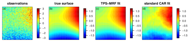
Figure 1: For simulated data (a) based on white noise added to a smooth true surface (b), (c) shows the posterior mean under the TPS-MRF model and (d) the posterior mean under a MRF model with a standard CAR neighborhood structure.

3.3 Spatial scales of discrepancy

3.3.1 Discrepancy scenarios and identifiability

One important goal of including the spatial discrepancy term is to understand the scales at which the proxy and the process of interest are well- and poorly-correlated. I posit a range of potential relationships and the implications for making use of proxy signal, as well as the implications of overly constraining the discrepancy process. These represent extreme scenarios, so real applications will likely involve a combination of scenarios.

• White noise discrepancy: the spatial structure in the proxy mirrors the focal process but there is fine-scale discrepancy at the scale of pixels that can be treated as white noise. Under this scenario, there is no need for $\phi(\cdot)$ given the white noise error structure, $\{e_{j}\}$. Smoothing over the proxy gives information about the process of interest.

• Small-scale discrepancy: the proxy accurately reflects the focal process at large scales, but there is smaller-scale spatially-correlated discrepancy. Under this scenario, models without a sufficiently flexible discrepancy term may treat the discrepancy as signal since it is not white noise, particularly when the proxy sample size overwhelms the gold standard observations. This allows the variation in the proxy to be explained by a spatial process rather than by white noise (with higher accompanying posterior density, analogous to a penalized likelihood setting), even at the expense of increasing the observation error variance. In contrast, with a flexible representation of $\phi(\cdot)$, the model can treat the discrepancy as having small-scale spatial dependence, thereby ignoring this component of variation in the proxy.
  Note that without dense gold standard data, the small-scale signal and noise in the proxy are not identifiable, but improved small-scale prediction may be achievable by attributing some of the small-scale variability in the proxy to the focal process. Estimation of $\beta_{1}$ thus involves a bias-variance tradeoff. Finally, unless there are large spatial gaps in the observations, it’s not clear if using the proxy to help estimate large-scale variation will improve upon simply smoothing the gold standard data.

• Large-scale discrepancy: the proxy accurately reflects small-scale variation in the focal process, but there is large-scale discrepancy. In this case, one can correct for discrepancy through $\phi(\cdot)$ (needing only moderate amounts of gold standard data) and predict small-scale variation in the focal process from small-scale variation in the proxy. In this case it would be appropriate to constrain $\phi(\cdot)$ to vary only at larger spatial scales.
  One potential difficulty is that discrepancy occurring at similar scales as the focal process can cause problems with identifiability. The attribution of variability between the discrepancy and the focal process is determined through a complicated tradeoff between the likelihood for the data, the likelihood for the proxy, and penalization of complexity via the spatial process priors. Unless one removes the large-scale variation in the proxy via a projection, discrepancy can ’leak’ into the focal process predictions, analogous to the bias occurring in the partial spline setting (Rice, 1986).

• Uninformative proxy: the proxy and focal process are at best weakly related at all scales. A model without a flexible discrepancy term may have trouble representing the proxy reasonably, with focal process predictions largely reflecting the proxy when the proxy sample size overwhelms the gold standard data as in the small-scale discrepancy scenario.

3.3.2 Spatial discrepancy diagnostic

To assess the spatial scales of the discrepancy term, I propose to use a spatial variogram-based diagnostic introduced by Jun and Stein (2004) for assessing numerical model performance relative to observations. They calculate variograms for the model output, observations, and model error (defined as model output minus observations). They propose the ratio of the model error variogram to the sums of the variograms for model output and observations as a distance-varying diagnostic of the spatial variation in the observations captured by the model output. If the model output and observations were independent, then the variogram of the error would be the sum of the variograms of output and observations, so the ratio would be one on average. My analog plugs the analogous quantities from the statistical model (2) into their diagnostic, using $\beta_{1}\mbox{\boldmath$L$}$ as the best estimate of the focal process, scaled to the units of the proxy:

$$M(d)=\frac{\mbox{Variog}(\mbox{\boldmath$\phi$};d)}{\mbox{Variog}(\mbox{\boldmath$\phi$}+\beta_{1}\mbox{\boldmath$L$};d)+\mbox{Variog}(\beta_{1}\mbox{\boldmath$L$};d)}.$$

$M(d)$ is interpreted as the proportion of the variation in the proxy that is accounted for by the discrepancy term, as a function of spatial scale, quantified by distance, $d$. The diagnostic has the following appealing extremal properties: when $\beta_{1}=0$ or if $\phi$ offsets all the variation in the focal process at a given scale, $M(d)=1$, indicating all of the variability in the proxy is explained by discrepancy. In the ideal situation when $\mbox{\boldmath$\phi$}=\mbox{\boldmath$0$}$ in general or has no variation at a given scale, then $M(d)=0$, indicating all of the variability in the proxy at the scale is explained by the process of interest.

3.4 Marginalization and MCMC sampling

The proposed model contains two latent processes that can trade off in explaining variation in the proxy. In addition there is cross-level dependence between each latent process and its hyperparameters. In such situations, marginalization over the process or joint sampling of a process and its hyperparameters (Rue and Held, 2005) are often used, when possible, to improve MCMC convergence and mixing. Here the high-dimensionality of the processes complicates matters further. The modeling approach allows for marginalization over the process values and then efficient computations based on sparse matrix manipulations, with details given in the Appendix. I marginalize first over the MRF(s) and then over any basis coefficients to produce a representation of the marginal posterior that can be calculated based on sparse matrix manipulations. Note that even with these efforts, sampling can be slow; for the mid-Atlantic and eastern U.S. analyses run times were on the order of 6 hours and 3-5 days, respectively. Much of this was required to achieve good mixing of the variance components for the MRF and spline basis coefficients without the use of informative priors.

4 Simulations

4.1 Methods

To assess the performance of the approach I fit a simplified model to simulated data under a variety of scenarios:

1. Large- and small-scale discrepancy present with $\beta_{1}=1$

2. Large- and small-scale discrepancy with $\beta_{1}=0$

3. No spatial discrepancy, $\beta_{1}=1$

4. Large-scale discrepancy only, $\beta_{1}=1$

5. Small-scale discrepancy only, $\beta_{1}=1$

6. Scenario 1 but with sparse observations ($n=40$)

I constructed the simulation to mimic the mid-Atlantic analysis, with similar number of gold-standard observations, $n=171$ (except for scenario 6) and including a subset of the covariates used there. The proxy is fully-observed over the entire 175x100 grid with no misalignment and with white noise discrepancy in all cases, but I calculate the likelihood only for the 15,157 land-based pixels. I used a GP with Matérn covariance, parameterized as in Banerjee et al. (2004), with $\nu=2$ and varying values of $\rho=1/\phi$ to simulate the residual spatial surface, $g$ (effective range: 340 grid cells), and (independently) the discrepancy, $\phi$, operating at two different scales (effective ranges: 413 and 24 grid cells) (when not zeroed out in a given scenario). Note that the surface generation model differs from the spatial process representations in the model. I included population density, elevation, road density in the two largest road size classes, and county average emissions as linear (on the log scale for the first two terms and square root scale for the other three) covariates for the focal process with coefficients of $0.2$, $-0.3$, $0.01$, $0.01$, and $0.1$. When fitting the model, I included road density in the third largest road size class rather than the first two largest to introduce some model misspecification. In addition, I introduced mismatch in some of the transformations between data generation and model fitting by using a linear function of elevation, truncated to a maximum of 500 m, a linear function of the road density, and the log transform of county emissions. As in the real analyses, I included local covariates to capture within-pixel variability. I generated local variability as a function of distances (m), $d_{1}$ and $d_{2}$, to the nearest major road in two size classes as $50d_{1}^{-0.77}+10d_{2}^{-0.77}$ . To fit the model I used linear terms of these distances, truncated at 10 and 500 m.

I carried out 10 replications, resampling the spatial surfaces and error terms. The variances of the different components were $0.55^{2}$ and $1.73^{2}$ for the normally-distributed proxy and observation white noise, respectively, $0.84^{2}$ for the empirical within-pixel variability from the two local covariates combined, $0.93^{2}$ for the empirical variability in the true process from the five land use covariates, $2.5^{2}$ for the residual spatial surface component of the true process, $1.64^{2}$ for the small-scale discrepancy, and $2.0^{2}$ for the large-scale discrepancy. For scenario 1, these settings produced correlations (spatially, over the land-based pixels) of the proxy and the focal process that varied (over the 10 replications) between 0.47 and 0.87 (median 0.67) (with a range of correlations of 0.76-0.88 when excluding the large-scale discrepancy), somewhat higher than correlations of 0.58 and 0.52 observed for the real proxies. In the replicates, larger correlations occurred when the residual spatial component of the true process and the large-scale discrepancy were more positively spatially correlated in a given realization, which occurs by chance because both vary at large spatial scale. Prior distributions were the same as described in the Appendix for the real analyses.

4.2 Results

I summarize the results based on mean square prediction error (MSPE) for the land-based pixels, averaged over the 10 replicates (Table 1). Note that it is difficult to compare MSPE values for different scenario-model combinations in the table because the variability across replicates is large compared to the differences between some of the combinations. To address this, in the text below, I compute standard errors of mean MSPE differences between scenario-model combinations based on paired replicates.

In general, the model is able to predict spatial variation in the true process reasonably well in these settings, but it does not exploit the information in the proxy effectively. Comparing the full model to a model that does not include the proxy, there is no improvement in MSPE. In scenarios 1, 3, 4, and 5, the mean difference (standard error of the difference) over 10 replications for full model minus reduced model is 0.02 (0.04), 0.10 (0.05), 0.09 (0.05), and 0.02 (0.04). Note that even for scenario 3, in which the proxy has no spatial discrepancy, the mean MSPE is larger for the full model. This indicates that lack of identifiability plays an important role here, with the full model having difficulty decomposing the spatial variation into signal and noise. Covariate coefficient estimates are quite sensitive to the inclusion of the proxy, indicating that there is substantial trading off of variability between the discrepancy, residual spatial, and covariate components of the model. In the full model, the posterior mean of $\beta_{1}$ generally ranges between 0.4 and 0.7, an attenuation relative to the true value of one, with the model attributing some of the signal in the proxy to the discrepancy term. In addition to these general identifiability issues, I note a more subtle difficulty in making use of the proxy to resolve small-scale spatial features (such as those induced in the simulations by the covariates). Small-scale variation not explained by the measured covariates can only be resolved as part of the pollution process through the residual spatial term, $g(\cdot)$. However, the spatial process prior, reflecting the natural Bayesian complexity penalty, penalizes complexity in $g(\cdot)$. Instead, the simulations indicate that the discrepancy term picks up the small-scale proxy signal, as the discrepancy term already needs to operate at a small scale to capture the small-scale proxy discrepancy.

Table 1: Average MSPE (standard error) for a variety of model structures for the six simulation scenarios.

	Simulation scenario
Model structure	1	2	3	4	5	6
Full model	1.09 (0.09)	1.03 (0.07)	1.17 (0.09)	1.16 (0.09)	1.09 (0.09)	1.67 (0.13)
No proxy data (Scenarios 1-5 are the same)	1.07 (0.08)					1.51 (0.11)
No discrepancy term	2.05 (0.11)	3.17 (0.17)	0.52 (0.05)	1.87 (0.12)	1.38 (0.08)	not run1
Discrepancy assumed large scale	1.83 (0.19)	2.36 (0.21)	0.84 (0.08)	0.88 (0.07)	1.80 (0.17)	not run1
Fixing $\beta_{1}=1$	0.90 (0.06)	1.43 (0.09)	0.88 (0.05)	0.88 (0.05)	0.90 (0.06)	not run1
Proxy used as covariate	1.06 (0.09)	1.09 (0.08)	0.86 (0.05)	0.96 (0.05)	1.04 (0.07)	1.57 (0.11)

¹These scenario-model combinations were not run as as they were expected to add little information to the simulation study.

Adding constraints to the model can improve the situation in some cases (Table 1). When there is no small-scale discrepancy, forcing $\phi(\cdot)$ to vary only at a large scale (by fixing $\kappa$ to be 1000) reduces MSPE relative to not constraining $\phi(\cdot)$ (mean differences of -0.33 (0.08) and -0.29 (0.12) for scenarios 3 and 4, respectively). Fixing $\beta_{1}=1$ also generally improves MSPE relative to not constraining $\beta_{1}$ (mean differences of -0.19 (0.08), -0.29 (0.09), -0.28 (0.09), and -0.19 (0.08) for scenarios 1, 3, 4, and 5, respectively). And not surprisingly, MSPE is lowest (0.52) in scenario 3 (no spatial discrepancy) when the discrepancy term is excluded. Unfortunately, in real applications, one does not know when the addition of constraints to improve identifiability is reasonable (although cross-validation can help to assess this). For example, when there is small-scale discrepancy, forcing $\phi(\cdot)$ to vary only at a large scale greatly increases MSPE relative to not constraining $\phi(\cdot)$ (mean differences of 0.75 (0.24), 1.33 (0.23), and 0.71 (0.23), for scenarios 1, 2, and 5 respectively), as does removing $\phi(\cdot)$ entirely (mean differences of 0.96 (0.16), 2.14 (0.20), 0.29 (0.11) for scenarios 1, 2, and 5, respectively).

Including the proxy as a covariate does not substantially reduce MSPE relative to not including the proxy when there is small-scale discrepancy (mean differences of -0.01 (0.03) and -0.03 (0.12) for scenarios 1 and 5, respectively) (Table 1). However, when there is no discrepancy or only large-scale discrepancy, then including the proxy as a covariate does reduce MSPE (mean differences of -0.22 (0.09) and -0.11 (.10) for scenarios 3 and 4, respectively, but note the large standard error for 4), with the model able to account for large-scale discrepancy in scenario 4 through $g(\cdot)$. The model can account for a large proportion of the spatial variation without the proxy, and the proxy is correlated with the measured covariates. Therefore, it is not surprising that using the proxy, which is essentially a measurement-error-contaminated variable, as a covariate is not always helpful.

In scenario 6, with the smaller sample size, the full model and the model using the proxy as a covariate are still unable to improve upon the reduced model without the proxy (mean differences of 0.15 (0.16) and 0.06 (0.08) relative to the model without the proxy) (Table 1). This suggests that even with sparse observations, discrepancy poses a challenge to taking advantage of the proxy when the reduced model has reasonable predictive ability ($R^{2}$ values ranging between 0.16 and 0.85 with a median of 0.68).

Note that the difficulty in exploiting the proxy occurs with correlations between the proxy and the truth that are on average higher than those seen in the real analyses of Section 5. This suggests that one needs a high-quality proxy when a model without the proxy performs reasonably well on its own. In the presence of discrepancy, the model discounts the proxy (recall the attentuated estimates of $\beta_{1}$), but error in the proxy still ’leaks’ into the focal process inference. Whether this leakage outweighs any benefit of proxy signal for prediction depends in a complicated fashion on the amount of information available in the observations and the signal to noise ratio in the proxy. On a positive note, the simulations indicate that the model is able to screen out proxies that are not sufficiently informative, with little decrease in predictive performance, despite the imbalance between gold standard and proxy sample sizes. On a negative note, in the simulations neither the discrepancy nor $\beta_{1}$ vary with the covariates, which is not realistic in the air pollution context and would likely make it harder to take advantage of a proxy by introducing non-identifiability between the covariates and the discrepancy.

Finally, I briefly consider prediction uncertainty (for scenario 1). The full model and the model including the proxy as a covariate have somewhat smaller prediction standard deviations (averaged over the land-based pixels) than the model without the proxy (0.89 and 1.01 compared to 1.04), but coverage is also lower (0.86 and 0.90 compared to 0.91).

Fig. 2 shows the discrepancy scale diagnostic (Section 3.3.2) for the full model under each scenario. In general, there appears to be reasonable, but imperfect, information in the diagnostic, with the expected relationship with scale given the data generation for a given scenario. That is, when there is more discrepancy at large than small scales the ratio should increase with distance (scenario 4) and when there is more discrepancy at small than large scales, it should decrease (scenario 5). Unfortunately, even when there is no true discrepancy at a scale the diagnostic estimates discrepancy, which is caused by the identifiability problems. This suggests that one should treat the diagnostic as indicative, rather than conclusive, about the scales of discrepancy. Also, the diagnostic results suggest caution in interpreting the diagnostic at the shortest distances, given the drop in the diagnostic even for the scenarios with small scale discrepancy (scenarios 1 and 5).

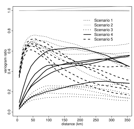
Figure 2: Discrepancy scale diagnostic for the model fit to simulated data (the first five of the 10 replications for clarity) under various scenarios: (1) large- plus small-scale discrepancy (thin dashed line), (2) uninformative proxy (thin grey line), (3) no spatial discrepancy (dotted line), (4) large-scale discrepancy only (thick line), and (5) small-scale discrepancy only.

5 Analysis of particulate matter

5.1 Spatial analysis of MODIS AOD in the mid-Atlantic region

I fit separate spatial models for each month of 2004 for the mid-Atlantic region with AOD from the MODIS instrument as the proxy. I used a regular four km grid of dimension 175 by 100 as the resolution of $L(\cdot)$, $g(\cdot)$, and $\phi(\cdot)$. MODIS AOD is misaligned with respect to this grid and for different satellite orbits on different days, the pixels shift spatially. Therefore, I considered the overlap of all the pixels in an orbit with the four km grid, assigning to each grid cell, $s_{j}$, the value of the MODIS pixel in which the cell centroid falls. Taking the retrievals assigned to each cell, I then averaged to the monthly level for each cell. More sophisticated approaches are possible (Mugglin et al., 2000), but for these purposes, this ad hoc realignment retained the essential character of the AOD retrievals and reduced computations. I attempted to account in part for informatively-missing AOD due to cloud cover (Paciorek et al., 2008) by including a smooth regression term, $\beta_{a}(x_{a})$, in the additive mean for the proxy, thereby making a missing-at-random assumption. $x_{a}$ is the average cloud cover over the month for each location, based on the cloud screen variable from the Geostationary Operational Environmental Satellite. $g(\cdot)$ was modeled using the thin plate spline mixed model representation. Distances to nearby roads in two road size classes, calculated for each monitor location, were used as smooth spline terms, $\beta_{y,p}(x_{y,p}),\,p=1,2$, while elevation, population density, road density in three road size classes, and area emissions were estimated at the four km resolution using a Geographic Information System and used as smooth spline terms, $\beta_{L,p}(x_{L,p}),\,p=1,\ldots 6$. Distance to point source emissions (those greater than five tons per year) was handled as a smooth function of distance, adding over the sources within 100 km of the observation (or grid cell), following the methodology of Paciorek and Liu (2011, Appendix D).

I considered both raw MODIS AOD and a ’calibrated’ MODIS AOD that adjusts off-line for the effects of boundary layer height and relative humidity, as well as large-scale temporal and spatial adjustments, based on comparison of co-located daily PM and AOD values (Paciorek and Liu, 2009). Results were similar and are presented here for raw MODIS AOD.

The estimated values of the regression coefficient, $\beta_{1}$, relating the proxy to the focal process were essentially zero in every month (Fig. 3c), indicating that the model found no relationship between the proxy and the PM process, ignoring the proxy in predicting PM. The spatial discrepancy plot indicates that the proxy is explained by the discrepancy term rather than the PM process at all scales (Fig. 3a). These results are consistent with those found in Paciorek and Liu (2009). Fig. 4 shows predictions from the model when excluding and including AOD, with very similar predictions. Correspondingly, (ten-fold) cross-validative predictive assessment indicated that including the proxy did not improve predictive performance (Table 2). (Yearly prediction appeared slightly worse when excluding the proxy, but this is likely within the uncertainty of the predictive assessment, which is difficult to quantify given the correlation structure of the data). Results were qualitatively similar when considering only held-out monitors in more rural areas, suggesting that AOD is not adding information in areas far from monitors (Table 2). In light of the simulation results, these results suggest that we are in the regime where the proxy is not sufficiently informative about the process of interest (relative to the strength of information in the gold standard data) to be able to exploit the information in the proxy indicated by the AOD-PM correlation of 0.58.

Figure 3: Discrepancy scale diagnostic plots (top row) and boxplots of posterior estimates of $\beta_{1}$ (bottom row) by month for analysis of MODIS AOD as the proxy in 2004 in the mid-Atlantic (left panel) and CMAQ as the proxy in 2001 in the eastern U.S. (right panels).

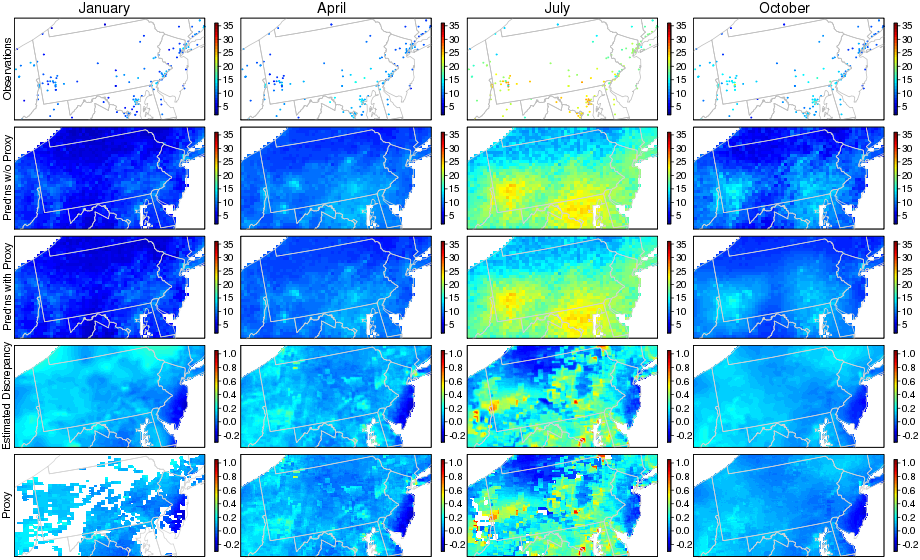
Figure 4: For the mid-Atlantic region of the U.S., PM observations (first row), model PM predictions excluding MODIS AOD (second row), model predictions including AOD (third row), estimated discrepancy in the model with AOD (fourth row), and AOD values (fifth row) for four months in 2004: January, April, July, and October (columns). White space in the land areas in the fifth row indicate AOD values missing because of cloud cover for all AOD retrievals in the month.

Table 2: Cross-validation predictive ability, $R^{2}$ (RMSPE), for monthly and yearly (average of the 12 monthly values) predictions, with and without proxy information, over the spatio-temporal domains of the analyses.

Time scale	Proxy inclusion	mid-Atlantic, 2004, MODIS AOD	eastern U.S., 2001, CMAQ
All monitors
Monthly prediction1	With proxy	0.806 (1.80)	0.827 (1.71)
	Without proxy	0.808 (1.79)	0.826 (1.72)
Yearly prediction2	With proxy	0.667 (1.00)3	0.800 (1.21)
	Without proxy	0.650 (1.03)3	0.835 (1.09)
Monitors generally isolated from other monitors4
Monthly prediction1	With proxy	0.830 (1.73)	0.739 (2.12)
	Without proxy	0.830 (1.72)	0.781 (1.94)
Yearly prediction2	With proxy	0.669 (1.17)	0.710 (1.58)
	Without proxy	0.624 (1.25)	0.826 (1.22)

¹ Including monthly averages based on at least five daily observations. ²Including yearly averages (averages of monthly values) based on at least nine months with at least five daily observations. ³ Excludes one site outside Pittsburgh just downwind of a major industrial facility. ⁴ Monitors in four km grid cells with fewer than 187.5 people per square km=3000 people per cell.

5.2 Spatial analysis of CMAQ output in the eastern United States

I fit separate monthly spatial models for 2001 for the entire eastern U.S. with CMAQ output as the proxy. For this analysis, I extended the four km grid over the the eastern U.S. (roughly the area east of $100^{{}^{\circ}}$W longitude), giving a grid of dimension 669 by 677. I used the 36 km CMAQ grid of dimension 73 by 77 for $\phi(\cdot)$. For this larger domain with more complexity in the pollution surface, I represented $g(\cdot)$ on this same 36 km grid using the TPS-MRF representation rather than the mixed model thin plate spline. The latter would have required a computationally burdensome increase in the number of basis coefficients. Note that I relied on the same covariates used in the mid-Atlantic analysis to represent small-scale residual spatial variability, such that representing $g(\cdot)$ on the 36-km CMAQ grid is sufficient, based on posterior assessment of the scale of $g(\cdot)$. To calculate the PM likelihood I used the covariate values for the four km grid cell that each observation falls in, while using the value of $g$ from the 36 km grid cell the observation falls in. For the CMAQ likelihood, the CMAQ value for a given 36 km grid cell was related to the covariate effects on the four km grid by weighted averaging, with weights based on the overlap between a CMAQ grid cell and the four km grid cells.

$\beta_{1}$ was estimated to be large (between three and seven), with $\phi$ strongly negatively correlated with $L$ and with $\phi$ having very large negative values to offset the large positive values of $\beta_{1}\mbox{\boldmath$L$}$. This appeared to be driven by CMAQ overpredicting in some urban areas, with CMAQ estimating the urban to rural gradient as being much stronger than apparent in the observations. $\phi$ then adjusts for the impact outside urban areas of large values of $\beta_{1}$, highlighting the lack of identifiability between the discrepancy and the PM process. To address this in an ad hoc manner and identify $\phi$ as the orthogonal variation in the proxy not accounted for in the PM process, I carried out an ad hoc orthogonalization of $\phi$ and $L$ within each step of the MCMC. While a formal orthogonality constraint on $\phi$ and $L$ is technically appealing, this simple approach was effective in practice, and predictive results were similar with and without the orthogonalization.

Using this orthogonalized specification, the estimated values of $\beta_{1}$ were generally near one, as one would hope (Fig. 3d). Somewhat more of the variability in CMAQ at larger scales was associated with the PM process than variability at smaller scales, suggesting that CMAQ is better able to resolve regional variability than more local variability (Fig. 3b). This is consistent with the discrepancy surfaces shown in Fig. 5, which include hotspots at the scale of states or portions of states that show no evidence of being real hotspots based on the observations, such as over Iowa/southern Minnesota and eastern North Carolina. Use of CMAQ as a proxy did not improve predictive ability (Table 2).

Considered in light of the simulation results, these results suggest that we are again in the regime where the proxy is not sufficiently informative about the process of interest (relative to the strength of information in the gold standard data) to be able to exploit the information in the proxy indicated by the CMAQ-PM correlation of 0.52. Given the apparent impact of extreme CMAQ predictions, further model refinement, such as letting $\beta_{1}$ vary with covariates such as population density, might improve our ability to extract information from the proxy.

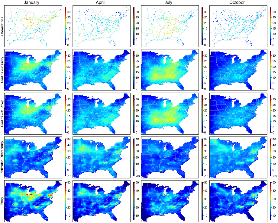
Figure 5: PM observations (first row), model PM predictions, excluding CMAQ (second row), model predictions including CMAQ (third row), estimated CMAQ discrepancy (fourth row), and CMAQ values (fifth row) for four months in 2001: January, April, July, and October (columns). Note that the scale for the CMAQ values is different than for the PM observations. Also note that in January, some CMAQ values larger than 50 $\mu g/m^{3}$ (up to 75 $\mu g/m^{3}$) are truncated to 50 $\mu g/m^{3}$.

As a final assessment, I included CMAQ as a simple regression term, finding the cross-validation $R^{2}$ (RMSPE) to be 0.849 (1.60) for monthly prediction and 0.849 (1.05) for yearly prediction, both slightly better than modeling without the proxy (Table 2) but suggesting that there is limited additional information given the other terms in the model. Similarly modest improvements were seen when restricting to more rural sites. The posterior mean regression coefficients for CMAQ-estimated PM were between 0.48 and 0.89 for the 12 months, with the average of those 12 posterior means being 0.67.

I also considered whether CMAQ might be more helpful in a setting with sparse observations by artificially using only 100 monitors as the PM dataset, but found that prediction for the remaining monitor locations was very poor, consistent with the simulation results, because the model was not able to adjust for the CMAQ discrepancy as well as with more dense data.

6 Discussion

The model developed here is a spatial latent variable model, in which the proxy is decomposed into signal for the process of interest and noise, which raises the obvious concern of identifiability. Sufficient gold standard observations are required for the implicit calibration of the proxy that is done within the model fitting. The penalized model identifies the discrepancy and the focal process based on a tradeoff between goodness of fit for the observations and for the proxy values and penalization of the latent spatial processes. This tradeoff is likely quite sensitive to model specification (note the trading off that occurred in the CMAQ analysis) and to the relative richness of observation and proxy data. The limited identifiability of the spatial processes in the model helps to explain the difficulty in exploiting the proxies seen in the simulations and the real analyses. Large-scale discrepancy occurring at a similar scale as the process of interest can leak into the estimated process. This stands in contrast to regression models in which fitting involves a projection that fully filters out the effect of covariates included for confounding control. When there is both discrepancy and signal in the proxy at smaller scales, the model has no way to distinguish these based on sparse observations. The discrepancy necessarily distorts the predictions. One can interpret the regression coefficient that relates the focal process and the proxy as a shrinkage parameter that weights the impact of the proxy on the focal process in the context of a complicated bias-variance tradeoff. Whether the proxy can improve prediction depends on the relative strength of the signal and noise in the proxy and the strength of information in the observations.

Despite these concerns about identifiability and sensitivity to model structure, the decomposition of signal and noise is a fundamental task when using proxies. One doesn’t know the quality of the proxy or the structure of any discrepancy and must assess this, ideally as a function of scale. As in the computer models literature (Bayarri et al., 2007), the lack of identifiability in the modeling follows from the scientific context. In contrast, a priori constraints on the flexibility of the discrepancy process incorporated into some data fusion approaches make strong assumptions about proxy quality. The model presented here attempts to assess proxy quality and to make use of available information in the proxy without prejudging that spatial correlation in the proxy reflects spatial signal for the process of interest. The results highlight the difficulty in actually improving predictions when including proxy information for which discrepancy is a concern and the need for new approaches that do not make strong assumptions about proxy quality but are better able to exploit information in the proxy.

The model accounts for errors and local variability in the observations, as well as spatial and temporal misalignment between observations and proxy. This should help to avoid concluding that a proxy is not helpful because of noise or fine-scale variability in the ’gold standard’, but I cannot completely rule out this possibility. However, I note that comparisons of daily maps of proxy values and observations indicate a great deal of mismatch between the two, of particular note on days when the observations show large-scale variation but little local variation. On such days the patterns in true PM are well-identified from the observations, yet the proxies often did a poor job of capturing that variation. It is possible that the proxy variables might add useful information in the absence of the GIS-based covariates, but part of the purpose of the covariates is to account for local variation in the observations that contributes to discrepancy between proxy and observations. Local variation that is not accounted for in the model structure is likely to mask any real relationship between the proxy and the true process of interest at the grid scale and may lead to discounting real information in the proxy.

As noted by a referee, it may seem curious to use a MRF representation in a context in which spatial scale is critical, given the lack of a spatial range parameter in the MRF. A recently-developed alternative to the TPS-MRF is the MRF approximation to GPs in the Matérn class (Lindgren et al., 2011). However, even GP approaches only explicitly model variation at a single scale. (Note they will also follow larger-scale variation except in data gaps.) To what extent might the limitations of the TPS-MRF prevent us from better exploiting the proxy? When there is large-scale discrepancy or no discrepancy, there is no reason to think that a GP or multiresolution model for the discrepancy would do any better in handling the identifiability problem. However, when only small-scale discrepancy is present, a multiresolution approach that imposes identifiability based on differentiating spatial scales might do a better job of preventing large-scale signal from being represented in the discrepancy term. More exploration of multiresolution approaches would be worthwhile, but they seem unlikely to deal substantially better with identifiability issues when the signal and noise vary at similar scales.

Rather than treating proxy information as data, Berrocal et al. (2010) proposed instead to regress on the proxy, which also greatly reduces computational complexity. In the simulations, I found that regressing on the proxy in some cases (no discrepancy or large-scale discrepancy only) improved predictive ability and in others (when small-scale discrepancy was present) had little effect. (Note that the presence of covariates in my settings likely decreases the potential for improvements from including the proxy, in comparison with the improved prediction seen in Berrocal et al. (2010) in a scenario without covariates.) So if one is purely interested in prediction and not in understanding the structure of the proxy, a simple regression approach may be best. An important drawback is that for proxies such as remote sensing retrievals affected by cloud cover, missing observations are a problem. This then requires an imputation of some sort, bringing one back to modeling the proxy.

The second potential drawback is more subtle and involves difficulties in decomposing the proxy into scales when the relationship with the process of interest varies by scale. If the proxy captures small-scale patterns well, but misses large-scale patterns, then the additive spatial process term used in Berrocal et al. (2010) can adjust for this discrepancy, leveraging the proxy to improve prediction of small-scale variation, a phenomenon seen also in my simulations. Concern arises when the proxy captures large-scale patterns well, but the small-scale patterns in the proxy are predominantly noise, a plausible scenario in applications. In such a setting, the model may estimate a large regression coefficient for the proxy because of the large-scale association. The resulting prediction will be reasonable at the large scale but will also include all the small-scale spatial discrepancy in the proxy, which will be interpreted by the analyst as signal, with the proxy assumed to be of high quality at small scales. The additive spatial process in the model will not be able to correct for this small-scale discrepancy because of the sparsity of the gold standard observations relative to the proxy. Alternatively, the small-scale discrepancy in the proxy may act as measurement error, causing attenuation in the regression coefficient and limiting any information gain from the large-scale signal in the proxy. One would like to carry out a decomposition of the scales of variability in the proxy, but the regression approach conditions on all the scales of the proxy.

From an interpretation standpoint, the approach proposed in this work cleanly distinguishes between discrepancy and signal in principle, albeit not in practice. A simpler alternative would be to explicitly decompose the proxy into two or more scales and include each component as a separate regression term, allowing the model to learn which scales are correlated with the observations. One might successively smooth the proxy with spatial smooth terms with fixed degrees of freedom or use kernel average predictors, as suggested in Heaton and Gelfand (2011).

Appendix: Model structures and fitting details

Spatial model structure for the mid-Atlantic analysis

The basic model is a model with two likelihoods and additive mean terms, in particular

$$Y \sim \mathcal{N}_{n_{Y}}(\mbox{\boldmath$Z$}_{y}\mbox{\boldmath$b$}_{y}+\mbox{\boldmath$Z$}_{L}\mbox{\boldmath$b$}_{L}+\mbox{\boldmath$P$}_{\delta}\mbox{\boldmath$\delta$},\mbox{\boldmath$V$}_{Y})$$

$$A \sim \mathcal{N}_{n_{A}}(\mbox{\boldmath$P$}_{\phi}\mbox{\boldmath$\phi$}+\mbox{\boldmath$Z$}_{a}\mbox{\boldmath$b$}_{a}+\beta_{1}\mbox{\boldmath$P$}_{A}\mbox{\boldmath$Z$}_{L}\mbox{\boldmath$b$}_{L},\mbox{\boldmath$V$}_{A})$$

$$\delta \sim \mathcal{N}(\mbox{\boldmath$0$},\sigma_{h}^{2}\mbox{\boldmath$I$})$$

$$\phi \sim \mathcal{N}_{m-3}(\mbox{\boldmath$0$},(\kappa\mbox{\boldmath$Q$})^{-})$$

$$\mbox{\boldmath$b$}=\{\mbox{\boldmath$b$}_{y},\mbox{\boldmath$b$}_{L},\mbox{\boldmath$b$}_{a}\} \sim \mathcal{N}(\mbox{\boldmath$0$},\mbox{\boldmath$\Lambda$})$$

where $\mbox{\boldmath$Z$}_{y}\mbox{\boldmath$b$}_{y}$ is the matrix representation of $\sum_{p}\beta_{y,p}(x_{y,p})$ and $\mbox{\boldmath$Z$}_{L}\mbox{\boldmath$b$}_{L}$ is the matrix representation of $\sum_{p}\beta_{L,p}(x_{L,p})+g(s)$ with $\mbox{\boldmath$b$}_{L}$ the collection of combined coefficients for the regression smooths and the spatial term, as well as including an intercept for $Y$. Similarly, $\mbox{\boldmath$Z$}_{a}\mbox{\boldmath$b$}_{a}$ represents the influence of explanatory variables for the proxy unrelated to latent PM (cloud cover in the case of the AOD model). $\delta$ are site-specific effects that account for correlation between monitors placed at the same site. I denote the variance of $\phi$ using the generalized inverse to indicate that the prior is proper in an $m-3$ dimensional space based on the construction of the TPS-MRF, fixing the mean and coefficients for linear terms of the spatial coordinates to zero. In the sampling, the three parameters are identified by the likelihood for $A$, so I sample these parameters implicitly as part of $\phi$ and therefore omit a separate intercept for $A$. Given the limited number of observation locations, I use five knots for each regression smooth and 55 knots for the spatial residual. Knots were placed either uniformly over the range of covariate values or at equally-spaced quantiles to achieve reasonable spread over the covariate spaces, but given the use of penalized splines, results should be robust to the exact placement of knots. $\Lambda$ is the prior covariance matrix of $b$ (non-informative for the fixed effect components and with exchangeable priors amongst the coefficients for a given regression smooth term, following Ruppert et al. (2003)).

I integrate over the conditional normal distribution of $\phi$, with mean $\mbox{\boldmath$M$}_{\phi}=\mbox{\boldmath$V$}_{\phi}(\mbox{\boldmath$P$}_{A}^{T}\mbox{\boldmath$V$}_{A}^{-1}(\mbox{\boldmath$A$}-\mbox{\boldmath$Z$}_{a}\mbox{\boldmath$b$}_{a}-\mbox{\boldmath$P$}_{A}\mbox{\boldmath$Z$}_{L}\mbox{\boldmath$b$}_{L}))$ and variance $\mbox{\boldmath$V$}_{\phi}=(\mbox{\boldmath$P$}_{\phi}^{T}\mbox{\boldmath$V$}_{A}^{-1}\mbox{\boldmath$P$}_{\phi}+\kappa\mbox{\boldmath$Q$})^{-1}$ to obtain

$$\mbox{\boldmath$A$}\sim\mathcal{N}_{n_{A}-3}(\mbox{\boldmath$Z$}_{a}\mbox{\boldmath$b$}_{a}+\beta_{1}\mbox{\boldmath$P$}_{A}\mbox{\boldmath$Z$}_{L}\mbox{\boldmath$b$}_{L},\mbox{\boldmath$\Sigma$}_{A}).$$

Here $\mbox{\boldmath$\Sigma$}_{A}^{-1}=\mbox{\boldmath$V$}_{A}^{-1}-\mbox{\boldmath$V$}_{A}^{-1}\mbox{\boldmath$P$}_{\phi}\mbox{\boldmath$V$}_{\phi}\mbox{\boldmath$P$}_{\phi}^{T}\mbox{\boldmath$V$}_{A}^{-1}$ and $|\mbox{\boldmath$\Sigma$}_{A}|^{-\frac{1}{2}}$ can be expressed as

$$\frac{1}{|\mbox{\boldmath$\Sigma$}_{A}|^{\frac{1}{2}}}=\frac{\kappa^{\frac{m-3}{2}}|\mbox{\boldmath$Q$}|^{\frac{1}{2}}}{|\mbox{\boldmath$V$}_{A}|^{\frac{1}{2}}|\mbox{\boldmath$V$}_{\phi}^{-1}|^{\frac{1}{2}}}.$$

Note that the impropriety in the prior for $\phi$ carries over into this marginal likelihood for $A$, resulting in $m-3$ rather than $m$ in the exponent of $\kappa$ and in $\mbox{\boldmath$\Sigma$}_{A}^{-1}$ being singular, with three zero eigenvalues, but the subsequent calculations all involve $\mbox{\boldmath$\Sigma$}_{A}^{-1}$ so no inversion is needed. Equivalently, I do not have a legitimate data-generating model for $A$ because of the prior impropriety. Information from three of the linear combinations in the quadratic form of the marginal likelihood contribute zero to the marginal likelihood because the variance for those combinations is infinite. I can avoid calculating the non-existent determinant of $Q$ because this is a constant with respect to the model parameters. Note that the impropriety is analogous to that in the marginal likelihood obtained from integrating over the mean in a simple normal mean problem with an improper prior for the mean.

I then integrate over the joint distribution for $b$, where I construct $\mbox{\boldmath$Z$}_{Y}$ and $\mbox{\boldmath$Z$}_{A}$ such that $\mbox{\boldmath$Z$}_{Y}\mbox{\boldmath$b$}=\mbox{\boldmath$Z$}_{y}\mbox{\boldmath$b$}_{y}+\mbox{\boldmath$Z$}_{L}\mbox{\boldmath$b$}_{L}$ and $\mbox{\boldmath$Z$}_{A}\mbox{\boldmath$b$}=\mbox{\boldmath$Z$}_{a}\mbox{\boldmath$b$}_{a}+\mbox{\boldmath$P$}_{A}\mbox{\boldmath$Z$}_{L}\mbox{\boldmath$b$}_{L}$ by adding columns with all zeroes as necessary. The conditional distribution for $b$ is normal with mean, $\mbox{\boldmath$M$}_{b}=\mbox{\boldmath$V$}_{b}(\mbox{\boldmath$Z$}_{Y}^{T}\mbox{\boldmath$V$}_{Y}(\mbox{\boldmath$Y$}-\mbox{\boldmath$P$}_{\delta}\mbox{\boldmath$\delta$})+\mbox{\boldmath$Z$}_{A}^{T}\mbox{\boldmath$\Sigma$}_{A}^{-1}\mbox{\boldmath$A$})$ and $\mbox{\boldmath$V$}_{b}=(\mbox{\boldmath$Z$}_{Y}^{T}\mbox{\boldmath$V$}_{Y}^{-1}\mbox{\boldmath$Z$}_{Y}+\mbox{\boldmath$Z$}_{A}^{T}\mbox{\boldmath$\Sigma$}_{A}^{-1}\mbox{\boldmath$Z$}_{A}+\mbox{\boldmath$\Lambda$}^{-1})^{-1}$. I collect the remaining parameters as $\mbox{\boldmath$\theta$}=\{\beta_{1},\sigma_{\mbox{\scriptsize{sub}}}^{2},\sigma_{\delta}^{2},\sigma_{\epsilon}^{2},\sigma_{A}^{2},\sigma_{\alpha}^{2},\mbox{\boldmath$\sigma$}_{b,L}^{2},\mbox{\boldmath$\sigma$}_{b,a}^{2},\mbox{\boldmath$\sigma$}_{b,y}^{2},\kappa\}$ where the variance components, $\mbox{\boldmath$\sigma$}_{b,y}^{2}$, $\mbox{\boldmath$\sigma$}_{b,L}^{2}$, and $\mbox{\boldmath$\sigma$}_{b,a}^{2}$, are vectors with one variance component for each smooth regression term in a given sum of regression smooths and $\sigma_{\mbox{\scriptsize{sub}}}^{2}$, $\sigma_{\delta}^{2}$, $\sigma_{\epsilon}^{2}$, $\sigma_{A}^{2}$, and $\sigma_{a}^{2}$ are parameters used to construct $\mbox{\boldmath$V$}_{Y}$ and $\mbox{\boldmath$V$}_{A}$, described below. The marginal posterior for the remaining parameters and $\delta$ is

$$P(\mbox{\boldmath$\theta$},\mbox{\boldmath$\delta$}|\mbox{\boldmath$A$},\mbox{\boldmath$Y$}) \propto |\mbox{\boldmath$\Lambda$}|^{-\frac{1}{2}}|\mbox{\boldmath$V$}_{Y}|^{-\frac{1}{2}}|\mbox{\boldmath$\Sigma$}_{A}|^{-\frac{1}{2}}|\mbox{\boldmath$V$}_{b}|^{\frac{1}{2}}P(\mbox{\boldmath$\delta$})P(\mbox{\boldmath$\theta$})\cdot$$ (3)

$$\exp\left(-\frac{1}{2}\left((\mbox{\boldmath$Y$}-\mbox{\boldmath$P$}_{\delta}\mbox{\boldmath$\delta$})^{T}\mbox{\boldmath$V$}_{Y}^{-1}(\mbox{\boldmath$Y$}-\mbox{\boldmath$P$}_{\delta}\mbox{\boldmath$\delta$})+\mbox{\boldmath$A$}^{T}\mbox{\boldmath$\Sigma$}_{A}^{-1}\mbox{\boldmath$A$}-\mbox{\boldmath$M$}_{b}^{T}\mbox{\boldmath$V$}_{b}^{-1}\mbox{\boldmath$M$}_{b}\right)\right),$$

which I use to sample $\theta$ via blocked Metropolis. Depending on the model, in some cases I use a single block and in other cases subblocks. I use adaptive MCMC to tune the proposal covariance matrix throughout the chain (Andrieu and Thoms, 2008).

The key computational impediments involve the determinant of $\mbox{\boldmath$V$}_{\phi}^{-1}$, which can be calculated based on sparse matrix operations since both of its components are sparse; note that $\mbox{\boldmath$P$}_{\phi}$ is a simple sparse mapping matrix assigning elements of $\phi$ to the proxy values. Next $\mbox{\boldmath$V$}_{b}$ is a dense matrix whose size corresponds to the number of basis coefficients, which can be computationally burdensome when I use a large number of knots for $g$ or the total number of knots used for all the regression smooth terms is large. Finally, I must compute $\mbox{\boldmath$\Sigma$}_{A}^{-1}\mbox{\boldmath$A$}$ and $\mbox{\boldmath$\Sigma$}_{A}^{-1}\mbox{\boldmath$Z$}_{A}$, the latter being more burdensome because $\mbox{\boldmath$Z$}_{A}$ is a matrix with as many non-zero columns as there are coefficients in $\{\mbox{\boldmath$b$}_{a},\mbox{\boldmath$b$}_{L}\}$. Considering the representation of $\mbox{\boldmath$\Sigma$}_{A}^{-1}$, note that I can easily compute $\mbox{\boldmath$V$}_{A}^{-1}\mbox{\boldmath$Z$}_{A}$ and then $\mbox{\boldmath$P$}_{\phi}^{T}\mbox{\boldmath$V$}_{A}^{-1}\mbox{\boldmath$Z$}_{A}$ because $\mbox{\boldmath$V$}_{A}^{-1}$ is diagonal and $\mbox{\boldmath$P$}_{\phi}^{T}$ is sparse. Next I use sparse matrix operations to solve the system of equations $\mbox{\boldmath$V$}_{\phi}\mbox{\boldmath$P$}_{A}^{T}\mbox{\boldmath$V$}_{A}^{-1}\mbox{\boldmath$Z$}_{A}$ (recall that I calculate $\mbox{\boldmath$V$}_{\phi}^{-1}$ quickly as the sparse matrix sum of two sparse matrices). I use the spam package in R for sparse matrix calculations.

Given the posterior for the remaining parameters (3), I can derive the closed form normal conditional distribution for $\delta$, which has mean and variance,

$$\mbox{\boldmath$M$}_{\delta} = \mbox{\boldmath$V$}_{\delta}(\mbox{\boldmath$P$}_{\delta}^{T}\mbox{\boldmath$V$}_{Y}^{-1}\mbox{\boldmath$Y$}-\mbox{\boldmath$P$}_{\delta}^{T}\mbox{\boldmath$V$}_{Y}^{-1}\mbox{\boldmath$Z$}_{Y}\mbox{\boldmath$V$}_{b}(\mbox{\boldmath$Z$}_{Y}^{T}\mbox{\boldmath$V$}_{Y}^{-1}\mbox{\boldmath$Y$}+\mbox{\boldmath$Z$}_{A}^{T}\mbox{\boldmath$\Sigma$}_{A}^{-1}\mbox{\boldmath$A$}))$$

$$\mbox{\boldmath$V$}_{\delta}^{-1} = \sigma_{\delta}^{2}\mbox{\boldmath$I$}+\mbox{\boldmath$P$}_{\delta}^{T}\mbox{\boldmath$V$}_{Y}^{-1}\mbox{\boldmath$P$}_{\delta}-\mbox{\boldmath$P$}_{\delta}^{T}\mbox{\boldmath$V$}_{Y}^{-1}\mbox{\boldmath$Z$}_{Y}\mbox{\boldmath$V$}_{b}\mbox{\boldmath$Z$}_{Y}^{T}\mbox{\boldmath$V$}_{Y}^{-1}\mbox{\boldmath$P$}_{\delta}.$$

Sampling from this distribution efficiently involves sparse matrix calculations similar to those just described.

Posterior samples of $\phi$ and $b$ can be drawn off-line from the conditional distributions indicated above; I choose to draw them every 10 MCMC iterations.

$\mbox{\boldmath$V$}_{Y}$ is modeled using a diagonal heteroscedastic variance, $(\mbox{\boldmath$V$}_{Y})_{ii}=\sigma_{\epsilon}^{2}/n_{i}+k(n_{i})\sigma_{\mbox{\scriptsize{sub}}}^{2}$ where the first term is the variance of the sum of independent daily instrument errors. The second reflects subsampling variability in the average of $n_{i}$ instrument-error-free daily values relative to the average of the error-free daily values over all the days in the month, $\mbox{Var}(\sum_{d\in\mbox{\scriptsize{subsample}}}L_{i,d}/n_{i}-\sum_{d}L_{i,d}/n_{\mbox{\scriptsize{month}}})$, under the simplifying assumption of independence between true daily pollution values, $L_{i,d}\stackrel{{\scriptstyle iid}}{{\sim}}\mathcal{N}(L(\mbox{\boldmath$s$}_{i}),\sigma_{\mbox{\scriptsize{sub}}}^{2})$, which gives $k(n_{i})=\frac{1}{n_{i}}-\frac{1}{n_{\mbox{\scriptsize{month}}}}$, where $n_{\mbox{\scriptsize{month}}}$ is the number of days in the month. Note that for simplicity I fixed $\sigma_{\epsilon}^{2}$ at $\widehat{\sigma_{\epsilon}^{2}}=1.5$, estimated in advance from co-located monitors, to enhance identifiability and because it has a small contribution to the overall error variance. For monitors not co-located with another monitor, I integrated over the prior for the $\delta$ values for those sites, which added a term, $\sigma_{h}^{2}$, to $(\mbox{\boldmath$V$}_{Y})_{ii}$. In contrast, I sampled the values of $\delta$ for sites with co-located monitors within the primary MCMC to avoid introducing off-diagonal elements into $\mbox{\boldmath$V$}_{Y}$ as this would have obviated some of the computational efficiencies in the calculations outlined above. For models involving CMAQ, which is available for all days, I take $\mbox{\boldmath$V$}_{A}=\sigma_{A}^{2}\mbox{\boldmath$I$}$. For models involving AOD, I use a diagonal heteroscedastic variance analogous to $\mbox{\boldmath$V$}_{Y}$ that reflects the number of daily values in each monthly average, plus a homoscedastic term reflecting the fundamental discrepancy between AOD and true PM: $(\mbox{\boldmath$V$}_{A})_{ii}=\sigma_{A}^{2}+k(n_{i})\sigma_{\alpha}^{2}$.

For simplicity and because I use monthly averages, I do not transform the PM values, in contrast to other work on PM (Smith et al., 2003; Yanosky et al., 2009), but log or square root transformations are good alternatives. For regression terms that represent sources, additivity on the original scale makes more sense while for modifying variables such as meteorology, log transformation to scale multiplicatively makes more sense. Achieving both in a single model is not easily accomplished. I note that the long right tail of CMAQ output may be accomodated through $\phi$ because the CMAQ output is spatially correlated. As in Paciorek et al. (2009), residuals from the various models indicated long-tailed behavior, reasonably characterized by t distributions with approximately five degrees of freedom, albeit with right skew. Predictive performance suggests that the influence of outliers is not extreme, but the use of a t distribution for the observation errors would be worth exploring. However, this would be somewhat difficult to do in the context of the additive error structure I derive above based on components of variability in the PM measurements.

I use several covariates calculated for individual cells at the four km grid level: elevation at the cell centroids, population density, and total length of roads in three road classes. Area PM emissions from the 2002 EPA National Emissions Inventory (NEI) are calculated as density of emissions per county, and the value for the county in which a grid cell centroid falls is assigned to the grid cell. Population density, road density, and area emissions are log-transformed to reduce sparsity and pull in extremely large values in the right tail, and I truncated the values of some outlying covariates to reduce extrapolation problems. I used the NEI point source emissions strength and location data in the flexible buffer modeling described in Paciorek and Liu (2011, Appendix D), creating a basis matrix that contributes columns to $\mbox{\boldmath$Z$}_{L}$. This matrix leverages the additive structure of the mixed model representation of a spline term to represent the effect of multiple point sources at a given receptor location (i.e., a monitor or prediction point) as the emission strength-weighted sum of a smooth distance effect evaluated for each individual source-receptor pair. The distance function is a universal function representing the effect of single source of unit strength on a receptor as a function of the distance between source and receptor and is estimated from the data. I calculate the source strength-weighted sum of distance-weighted contributions from fine PM primary source point emissions within a maximum distance (100 km) for each monitor, omitting sources emitting less than five tons in 2002. For the proxy likelihood and for prediction on the grid, I take a subgrid of 16 points within each grid box and calculate the average sum of contributions from the point emissions within 100 km of the points in the subgrid, as a simple approximation to the true integral of the point emission effect over the grid cell.

In general, the prior distributions for hyperparameters were non-informative, with normal priors with large variances (and also lower and upper bounds to prevent the MCMC from wandering in flat parts of the posterior) for location parameters and uniform priors on the standard deviation scale for scale parameters (Gelman, 2006), with large upper bounds. In all cases, the posterior distributions were much more peaked than the prior distributions and away from the bounds, except for some of the variance components for the coefficients of the regression smooths, which I restricted to avoid overly wiggly smooth terms. Further exploration of why these smooths tend toward less smooth functions than expected scientifically and on whether simple linear relationships would suffice, and might even improve out-of-sample prediction, would be worthwhile.

I ran the MCMC for 10,000 iterations during the burn-in and 25,000 subsequently, retaining every 10th iteration to reduce storage costs. I found reasonable convergence and mixing based on effective sample size calculations and trace plots. I did not run multiple chains for each month-validation set pair because of my use of multiple months and validation sets, noting that predictive performance also helps to justify the adequacy of the fitting.

Modifications for the eastern U.S. analysis

Details here generally follow those just described, but for computational efficiency, I represent $\phi$ and $g$ as TPS-MRFs on the $73\times 77=5621$ dimensional CMAQ grid over the eastern U.S., each with its own precision parameter. Covariate effects are represented on the original four km base grid (now of dimension $669\times 677=452,913$). Pre-computation of $\mbox{\boldmath$Z$}_{A}$ in advance of the MCMC involves the large matrix multiplication of a basis matrix and an averaging matrix that represents the weighted average of four km cells within each CMAQ pixel based on the amount of overlap. $\mbox{\boldmath$Z$}_{Y}$ also represents the product of a mapping matrix and the original basis matrices for the covariates. Given the relatively large sample size, for this model I use 10 rather than five knots for each regression smooth term.

The initial integration is over $\mbox{\boldmath$\phi$}^{*}=\{\mbox{\boldmath$g$},\mbox{\boldmath$\phi$}\}$ followed by integration over $b$, which no longer includes $\mbox{\boldmath$b$}_{g}$. The first integration is done by representing the joint likelihood as

$$\left(\begin{array}[]{c}\mbox{\boldmath$Y$}\\ \mbox{\boldmath$A$}\end{array}\right) \sim \mathcal{N}_{n_{Y}+n_{A}}\left(\left(\begin{array}[]{c}\mbox{\boldmath$Z$}_{Y}\\ \mbox{\boldmath$Z$}_{A}\end{array}\right)\mbox{\boldmath$b$}+\left(\begin{array}[]{cc}\mbox{\boldmath$P$}_{Y}&\mbox{\boldmath$0$}\\ \beta_{1}\mbox{\boldmath$P$}_{A}&\mbox{\boldmath$P$}_{A}\end{array}\right)\left(\begin{array}[]{c}\mbox{\boldmath$g$}\\ \mbox{\boldmath$\phi$}\end{array}\right)+\left(\begin{array}[]{c}\mbox{\boldmath$P$}_{\delta}\\ \mbox{\boldmath$0$}\end{array}\right)\mbox{\boldmath$\delta$},\left(\begin{array}[]{cc}\mbox{\boldmath$V$}_{Y}&\mbox{\boldmath$0$}\\ \mbox{\boldmath$0$}&\mbox{\boldmath$V$}_{A}\end{array}\right)\right),$$

followed by analogous calculations to those in the previous section to integrate over $b$ and determine the marginal posterior (up to the normalizing constant) for the remaining parameters and the conditional normal posterior for $\delta$ given the remaining parameters and the data. Note that $\mbox{\boldmath$P$}_{Y}$ and $\mbox{\boldmath$P$}_{A}$ simply map from the CMAQ grid cells to the observations and CMAQ values.

Some CMAQ pixels overlap four km cells entirely over water, and those cells have undefined covariate values. I treat the CMAQ value in a CMAQ pixel as reflecting the weighted average of $L(\cdot)$ from only the land-based four km grid cells, with weights in $\mbox{\boldmath$P$}_{A}$ summing to one for each CMAQ pixel. I do not include CMAQ values in the likelihood for CMAQ pixels with 60% or more overlap with four km cells that do not intersect land in the U.S.

For the point source emissions covariate, computational demands required that I consider only point sources emitting more than 10 tons per year within 50 km of a given location, with the integral approximation using a subgrid with four, rather than 16, points within each four km cell.

I ran the MCMC for 10,000 iterations during the burn-in and 20,000 subsequently, retaining every 10th iteration to reduce storage costs, again finding reasonable convergence and mixing.

References

- Andrieu and Thoms (2008) Andrieu, C. and J. Thoms (2008). A tutorial on adaptive MCMC. Statistics and Computing 18(4), 343–373.
- Banerjee et al. (2004) Banerjee, S., B. Carlin, and A. Gelfand (2004). Hierarchical Modeling and Analysis for Spatial Data. Boca Raton, Florida: Chapman & Hall.
- Banerjee et al. (2008) Banerjee, S., A. Gelfand, A. Finley, and H. Sang (2008). Gaussian predictive process models for large spatial data sets. Journal of the Royal Statistical Society: Series B (Statistical Methodology) 70(4), 825–848.
- Bayarri et al. (2007) Bayarri, M., J. Berger, R. Paulo, J. Sacks, J. Cafeo, J. Cavendish, C. Lin, and J. Tu (2007). A framework for validation of computer models. Technometrics 49(2), 138–154.
- Berrocal et al. (2010) Berrocal, V., A. Gelfand, and D. Holland (2010). A spatio-temporal downscaler for output from numerical models. Journal of Agricultural, Biological, and Environmental Statistics 15, 176–197.
- Besag and Mondal (2005) Besag, J. and D. Mondal (2005). First-order intrinsic autoregressions and the de Wijs process. Biometrika 92(4), 909–920.
- Crainiceanu et al. (2005) Crainiceanu, C., D. Ruppert, and M. Wand (2005). Bayesian analysis for penalized spline regression using WinBUGS. Journal of Statistical Software 14(14), 1–24.
- Cressie (1993) Cressie, N. (1993). Statistics for Spatial Data (Rev. ed.). New York: Wiley-Interscience.
- Fuentes and Raftery (2005) Fuentes, M. and A. Raftery (2005). Model evaluation and spatial interpolation by Bayesian combination of observations with outputs from numerical models. Biometrics 61(1), 36–45.
- Fuentes et al. (2008) Fuentes, M., B. Reich, and G. Lee (2008). Spatial-temporal mesoscale modelling of rainfall intensity using gauge and radar data. Annals of Applied Statistics 2, 1148–1169.
- Gelman (2006) Gelman, A. (2006). Prior distributions for variance parameters in hierarchical models (comment on article by Browne and Draper). Bayesian Analysis 1(3), 515–534.
- Heaton and Gelfand (2011) Heaton, M. and A. Gelfand (2011). Spatial regression using kernel averaged predictors. Journal of Agricultural, Biological, and Environmental Statistics 16, 233–252.
- Jun and Stein (2004) Jun, M. and M. Stein (2004). Statistical comparison of observed and CMAQ modeled daily sulfate levels. Atmospheric Environment 38(27), 4427–4436.
- Kammann and Wand (2003) Kammann, E. and M. Wand (2003). Geoadditive models. Applied Statistics 52, 1–18.
- Lindgren et al. (2011) Lindgren, F., H. Rue, and J. Lindström (2011). An explicit link between Gaussian fields and Gaussian Markov random fields: the stochastic partial differential equation approach. Journal of the Royal Statistical Society, Series B 73, 423–498.
- McMillan et al. (2010) McMillan, N., D. Holland, M. Morara, and J. Feng (2010). Combining numerical model output and particulate data using Bayesian space-time modeling. Environmetrics 21, 48–65.
- Mugglin et al. (2000) Mugglin, A., B. Carlin, and A. Gelfand (2000). Fully model-based approaches for spatially misaligned data. Journal of the American Statistical Association 95(451), 877–887.
- Paciorek and Liu (2009) Paciorek, C. and Y. Liu (2009). Limitations of remotely-sensed aerosol as a spatial proxy for fine marticulate matter. Environmental Health Perspectives 117, 904–909.
- Paciorek and Liu (2011) Paciorek, C. and Y. Liu (2011). Assessment and statistical modeling of the relationship between remotely-sensed aerosol optical depth and . Technical Report 00, Health Effects Institute Research Report.
- Paciorek et al. (2008) Paciorek, C., Y. Liu, H. Moreno-Macias, and S. Kondragunta (2008). Spatio-temporal associations between GOES aerosol optical depth retrievals and ground-level . Environmental Science and Technology 42, 5800–5806.
- Paciorek et al. (2009) Paciorek, C., J. Yanosky, R. Puett, F. Laden, and H. Suh (2009). Practical large-scale spatio-temporal modeling of particulate matter concentrations. Annals of Applied Statistics 3, 369–396.
- Rice (1986) Rice, J. (1986). Convergence rate for partially linear splined models. Statistics and Probability Letters 4, 203–208.
- Rue and Held (2005) Rue, H. and L. Held (2005). Gaussian Markov Random Fields: Theory and Applications. Boca Raton: Chapman & Hall.
- Ruppert et al. (2003) Ruppert, D., M. Wand, and R. Carroll (2003). Semiparametric Regression. Cambridge, U.K.: Cambridge University Press.
- Sahu et al. (2009) Sahu, S., A. Gelfand, and D. Holland (2009). Fusing point and areal level space-time data with application to wet deposition. Journal of the Royal Statistical Society: Series C (Applied Statistics) 59, 77–103.
- Smith et al. (2003) Smith, R., S. Kolenikov, and L. Cox (2003). Spatiotemporal modeling of PM2.5 data with missing values. Journal of Geophysical Research 108, D9004.
- Szpiro et al. (2010) Szpiro, A., P. Sampson, L. Sheppard, T. Lumley, S. Adar, and J. Kaufman (2010). Predicting intra-urban variation in air pollution concentrations with complex spatio-temporal dependencies. Environmetrics 21, 606–631.
- van Donkelaar et al. (2010) van Donkelaar, A., R. Martin, M. Brauer, R. Kahn, R. Levy, C. Verduzo, and P. Villeneuve (2010). Global estimates of exposure to fine particulate matter concentrations from satellite-based aerosol optical depth. Environmental Health Perspectives 118, 847–855.
- Yanosky et al. (2009) Yanosky, J., C. Paciorek, and H. Suh (2009). Predicting chronic fine and coarse particulate exposures using spatio-temporal models for the northeastern and midwestern U.S. Environmental Health Perspectives 117, 522–529.
- Yue and Speckman (2010) Yue, Y. and P. Speckman (2010). Nonstationary spatial Gaussian Markov random fields. Journal of Computational and Graphical Statistics 19, 96–116.