Observational constraints on phantom power-law cosmology

Abstract

We investigate phantom cosmology in which the scale factor is a power law, and we use cosmological observations from Cosmic Microwave Background (CMB), Baryon Acoustic Oscillations (BAO) and observational Hubble data, in order to impose complete constraints on the model parameters. We find that the power-law exponent is $\beta\approx-6.51^{+0.24}_{-0.25}$, while the Big Rip is realized at $t_{s}\approx 104.5^{+1.9}_{-2.0}$ Gyr, in 1$\sigma$ confidence level. Providing late-time asymptotic expressions, we find that the dark-energy equation-of-state parameter at the Big Rip remains finite and equal to $w_{DE}\approx-1.153$, with the dark-energy density and pressure diverging. Finally, we reconstruct the phantom potential.

I Introduction

Recent cosmological observations obtained by SNIa c1 , WMAP c2 , SDSS c3 and X-ray c4 indicate that the observable universe experiences an accelerated expansion. Although the simplest way to explain this behavior is the consideration of a cosmological constant c7 , the known fine-tuning problem 8 led to the dark energy paradigm. The dynamical nature of dark energy, at least in an effective level, can originate from a variable cosmological “constant” varcc , or from various fields, such is a canonical scalar field (quintessence) quint , a phantom field, that is a scalar field with a negative sign of the kinetic term Caldwell:2003vq ; phant , or the combination of quintessence and phantom in a unified model named quintom quintom . Finally, an interesting attempt to probe the nature of dark energy according to some basic quantum gravitational principles is the holographic dark energy paradigm holoext (although the recent developments in Horava gravity could offer a dark energy candidate with perhaps better quantum gravitational foundations Horawa ).

The advantage of phantom cosmology, either in its simple or in its quintom extension, is that it can describe the phantom state of the universe, that is when the dark energy equation-of-state parameter lies below the phantom divide $-1$, as it might be the case according to observations c1 . Additionally, a usual consequence of phantom cosmology in its basic form, is the future Big Rip BigRip or similar singularities BigRip2 , and thus one needs additional non-conventional mechanism if he desires to avoid such a possibility Sami:2003xv .

On the other hand power-law cosmology, where the scale factor is a power of the cosmological time, proves to be a very good phenomenological description of the universe evolution, since according to the value of the exponent it can describe the radiation epoch, the dark matter epoch, and the accelerating, dark energy epoch Kolb1989 ; Peebles:1994xt ; Nojiri:2005pu . Although it is tightly constrained by nucleosynthesis Sethi:1999sq ; Kaplinghat:1999 , considering late universe, it is found to be consistent with age of high-redshift objects such as globular clusters Lohiya:1997ti , with the SNIa data Sethi2005 ; Dev:2008ey , and with X-ray gas mass fraction measurements of galaxy clusters Allen2002 ; Zhu:2007tm . Furthermore, in the context of the power-law model, one can describe the gravitational lensing statistics Dev:2002sz , the angular size-redshift data of compact radio sources Alcaniz:2005ki , and the SNIa magnitude-redshift relation Dev:2002sz ; Sethi2005 .

In this work we desire to impose observational constraints on phantom power-law cosmology, that is on the scenario of a phantom scalar field along with the matter fluid in which the scale factor is a power law. In particular, we use cosmological observations from Cosmic Microwave Background (CMB), Baryon Acoustic Oscillations (BAO) and observational Hubble data ($H_{0}$), in order to impose complete constraints on the model parameters, focusing on the power-law exponent and on the Big Rip time.

This paper is organized as follows. In section II we construct the scenario of phantom power-law cosmology. In section III we use observational data in order to impose constraints on the model parameters, and in section IV we discuss the physical implications of the obtained results. Finally, section V is devoted to the conclusions.

II Phantom cosmology with Power-Law Expansion

In this section we present phantom cosmology under power-law expansion. Throughout the work we consider the homogenous and isotropic Friedmann-Robertson-Walker (FRW) background geometry with metric

$$ds^{2}=dt^{2}-a^{2}(t)\left[\frac{dr^{2}}{1-kr^{2}}+r^{2}d\Omega_{2}^{2}\right],$$ (1)

where $t$ is the cosmic time, $r$ is the spatial radius coordinate, $\Omega_{2}$ is the 2-dimensional unit sphere volume, and $k$ characterizes the curvature of 3-dimensional space of which $k=-1,0,1$ corresponds to open, flat and closed universe respectively. Finally, as usual, $a(t)$ is the scale factor.

The action of a universe constituted of a phantom field $\phi$, minimally coupled to gravity, reads phant :

$$S=\int d^{4}x\sqrt{-g}\left[\frac{R}{16\pi G}+\frac{1}{2}g^{\mu\nu}\partial_{\mu}\phi\partial_{\nu}\phi+V(\phi)+L_{\text{m}}\right],$$ (2)

where $V(\phi)$ is the phantom field potential, $R$ the Ricci scalar and $G$ the gravitational constant. The term $L_{\text{m}}$ accounts for the total (dark plus baryonic) matter content of the universe, which is assumed to be a barotropic fluid with energy density $\rho_{m}$ and pressure $p_{m}$, and equation-of-state parameter $w_{m}=p_{m}/\rho_{m}$. Finally, since we focus on small redshifts the radiation sector is neglected, although it could be straightforwardly included.

The Friedmann equations, in units where the speed of light is 1, write:

$$H^{2} = \frac{8\pi G}{3}\Big{(}\rho_{m}+\rho_{\phi}\Big{)}-\frac{k}{a^{2}}$$ (3)

$$\dot{H} = -4\pi G\Big{(}\rho_{m}+p_{m}+\rho_{\phi}+p_{\phi}\Big{)}+\frac{k}{a^{2}},$$ (4)

where a dot denotes the derivative with respect to $t$ and $H\equiv\dot{a}/a$ is the Hubble parameter. In these expressions, $\rho_{\phi}$ and $p_{\phi}$ are respectively the energy density and pressure of the phantom field, which are given by:

$$\rho_{\phi}=-\frac{1}{2}\dot{\phi}^{2}+V(\phi)$$ (6)

$$p_{\phi}=-\frac{1}{2}\dot{\phi}^{2}-V(\phi).$$

The evolution equation of the phantom field, describing its energy conservation as the universe expands, is

$$\dot{\rho}_{\phi}+3H(\rho_{\phi}+p_{\phi})=0,$$ (7)

or written equivalently in field terms:

$$\ddot{\phi}+3H\dot{\phi}-\frac{dV}{d\phi}=0.$$ (8)

Note that as we mentioned in the Introduction, in phantom cosmology the dark energy sector is attributed to the phantom field, that is $\rho_{DE}\equiv\rho_{\phi}$ and $p_{DE}\equiv p_{\phi}$, and thus its equation-of-state parameter is given by

$$w_{DE}\equiv\frac{p_{DE}}{\rho_{DE}}=\frac{p_{\phi}}{\rho_{\phi}}.$$ (9)

Finally, the equations close by considering the evolution of the matter density:

$$\dot{\rho}_{m}+3H(1+w_{m})\rho_{m}=0,$$ (10)

with straightforward solution

$$\rho_{m}=\frac{\rho_{m0}}{a^{n}},$$ (11)

where $n\equiv 3(1+w_{m})$ and $\rho_{m0}\geq 0$ is the value at present time $t_{0}$.

Lastly, note that we can extract two helpful relations, namely from (3) we obtain

$$\rho_{\phi}=\frac{3}{8\pi G}\Big{(}H^{2}-\frac{8\pi G}{3}\rho_{m}+\frac{k}{a^{2}}\Big{)},$$ (12)

while from (4),(6) we acquire

$$\dot{\phi}^{2}=\frac{1}{4\pi G}\Big{(}\dot{H}-\frac{k}{a^{2}}\Big{)}+\rho_{m}\frac{n}{3}.$$ (13)

Let us now incorporate the power-law behavior of the scale factor. In the case of quintessence cosmology, the power-law ansatz takes the usual form

$$a(t)=a_{0}\left(\frac{t}{t_{0}}\right)^{\beta},$$ (14)

with $a_{0}$ the value of the scale factor at present time $t_{0}$. However, in the case of phantom scenario, the power-law ansatz must be slightly modified, in order to acquire self-consistency. In particular, one rescales time as $t\rightarrow t_{s}-t$, with $t_{s}$ a sufficiently positive reference time, and thus the scale factor becomes Nojiri:2005vv ; Nojiri:2005pu :

$$a(t)=a_{0}\left(\frac{t_{s}-t}{t_{s}-t_{0}}\right)^{\beta},$$ (15)

while the Hubble parameter and its time-derivative read:

$$H(t)\equiv\frac{\dot{a}(t)}{a(t)}=-\frac{\beta}{t_{s}-t}$$ (16)

$$\dot{H}=-\frac{\beta}{(t_{s}-t)^{2}}.$$ (17)

Therefore, for $\beta<0$ we have an accelerating ($\ddot{a}(t)>0$) and expanding ($\dot{a}(t)>0$) universe, which possesses additionally a positive $\dot{H}(t)$ that is it exhibits super-acceleration Das:2005yj . That is, in phantom power-law cosmology, expansion is always accompanied by acceleration. Furthermore, with $\beta<0$, at $t=t_{s}$ the scale factor and the Hubble parameter diverge, that is the universe results to a Big Rip. These behaviors are common in phantom cosmology phant ; Briscese:2006xu and their realization is a self-consistency test of our work. On the other hand, note that the quintessence-ansatz (14) cannot lead to acceleration or to Big Rip and this was the reason for the introduction of the phantom power-law ansatz (15) in Nojiri:2005vv ; Nojiri:2005pu .

Having introduced the power-law ansatz that is suitable for phantom cosmology, we can easily extract the time-dependence of the various quantities, which re-expressed as functions of the redshift can be confronted by the observational data. In particular, substituting (11),(12), (13) in (6) we obtain

$$V(\phi)=\frac{3}{8\pi G}\left(H^{2}+\frac{\dot{H}}{3}+\frac{2k}{3a^{2}}\right)+\left(\frac{n-6}{6}\right)\frac{\rho_{m0}}{a^{n}}.$$ (18)

In the following we consider as usual the matter (dark plus baryonic) component to be dust, that is $w_{m}\approx 0$ or equivalently $n=3$. Thus, using the ansatz (15), and restoring the SI units using also $M_{\mathrm{P}}^{2}=\hbar c/8\pi G$, we obtain

$$V(t)=\frac{M_{\mathrm{P}}^{2}c}{\hbar}\left[\frac{3\beta^{2}-\beta}{(t_{s}-t)^{2}}+\frac{2kc^{2}(t_{s}-t_{0})^{2\beta}}{a_{0}^{2}(t_{s}-t)^{2\beta}}\right]-\frac{\rho_{m0}c^{2}}{2}\frac{(t_{s}-t_{0})^{3\beta}}{a_{0}^{3}(t_{s}-t)^{3\beta}}.$$ (19)

Additionally, solving equation (13) for the phantom field and inserting the power-law scale factor, gives

$$\phi(t)=\int\sqrt{\frac{2M_{\mathrm{P}}^{2}c}{\hbar}\left[-\frac{\beta}{(t_{s}-t)^{2}}-\frac{kc^{2}(t_{s}-t_{0})^{2\beta}}{a_{0}^{2}(t_{s}-t)^{2\beta}}\right]+\frac{\rho_{m0}c^{2}(t_{s}-t_{0})^{3\beta}}{a_{0}^{3}(t_{s}-t)^{3\beta}}}\,dt.$$ (20)

Finally, the time-dependence of the phantom energy density and pressure can be extracted from (6) and (6), using (19) and (20), namely:

$$\rho_{\phi}=\frac{M_{\rm P}^{2}c}{\hbar}\left[\frac{3\beta^{2}}{(t_{s}-t)^{2}}+\frac{3kc^{2}(t_{s}-t_{0})^{2\beta}}{a_{0}^{2}(t_{s}-t)^{2\beta}}\right]-\frac{\rho_{m0}c^{2}(t_{s}-t_{0})^{3\beta}}{a_{0}^{3}(t_{s}-t)^{3\beta}}$$ (21)

$$p_{\phi}=-\frac{M_{\rm P}^{2}c}{\hbar}\left[\frac{3\beta^{2}-3\beta}{(t_{s}-t)^{2}}\right]-\frac{\rho_{m0}c^{2}(t_{s}-t_{0})^{3\beta}}{2a_{0}^{3}(t_{s}-t)^{3\beta}},$$ (22)

and thus we can straightforwardly extract the time evolution of the dark energy equation-of-state parameter through (9) as $w_{DE}(t)={p_{\phi}(t)}/{\rho_{\phi}(t)}$. Note that at $t\rightarrow t_{s}$, apart from the scale factor, $\rho_{\phi}$ and $p_{\phi}$ diverge too, however $w_{DE}$ remains finite. This is exactly the Big Rip behavior according to the classification of singularities of BigRip2 .

All the aforementioned time-dependencies can be expressed in terms of the redshift $z$. In particular, since $1+z=a_{0}/a$, in phantom power-law cosmology we have

$$t=t_{s}-(t_{s}-t_{0})(1+z)^{-1/\beta}.$$ (23)

Therefore, using this relation we can extract the $z$-dependence of all the relevant quantities of the scenario at hand, which can then straightforwardly be confronted by the data.

III Observational constraints

In the previous section we presented the cosmological scenario in which the dark energy sector is attributed to a phantom scalar field, and where the scale factor is a power law of the cosmic time. Thus, in the present section we can proceed to confrontation with observations. In particular, we use Cosmic Microwave Background (CMB), Baryon Acoustic Oscillations (BAO) and Observational Hubble Data ($H_{0}$), in order to impose constraints on the model parameters, and especially to the power-law exponent $\beta$ and to the Big Rip time $t_{s}$. Finally, we first obtain our results using only the CMB-WMAP7 data Larson:2010gs , and then we perform a combined fit using additionally the BAO Percival:2009xn and $H_{0}$ ones ref:0905 .

We mention that in the present work we prefer not to use SNIa data as in the combined WMAP5+BAO+SNIa dataset Komatsu:2008hk . This is because the combined WMAP5 dataset uses SNIa data from Hicken:2009dk ; Kowalski:2008ez which do not include systematic error, and the cosmological parameters derived from the combined WMAP5 dataset also differ from those derived from other compilations of SNIa data Kessler:2009ys . Inclusion of the SNIa systematic error which is comparable to the its statistical error can significantly alter the value of the equation of state Komatsu:2010fb . Furthermore, recent analysis shows that the value of the equation-of-state parameter derived from two different light-curve fitters could be different from the one derived from two different datasets. This could make it difficult to identify if $w_{DE}$ is phantom, since its obtained values from the two fitters are different Bengochea:2010it . A very recent critics on SNIa data analysis has been presented in Vishwakarma:2010nc . Definitely the incorporation of SNIa data in constraining phantom cosmology is a subject that deserves further investigation.

Similarly to the non-phantom case Thepsuriya:2009wq , the exponent $\beta$ can be straightforwardly expressed as

$$\beta=-H_{0}(t_{s}-t_{0}),$$ (24)

where, as usual, we use the subscript 0 to denote the value of a quantity at present, and we moreover set $a_{0}$ to 1. Furthermore, we introduce the usual density parameter $\Omega_{m}\equiv 8\pi G\rho_{m}/(3H^{2})$, and we split $\Omega_{m}$ in its baryonic and cold dark matter part, $\Omega_{b}$ and $\Omega_{CDM}$ respectively ($\Omega_{m}=\Omega_{b}+\Omega_{CDM}$). Lastly, it proves convenient to introduce the critical density $\rho_{c}=3H^{2}/8\pi G$, and thus we can use the relation $\rho_{m0}=\Omega_{m0}\rho_{c0}$.

In a general, non-flat geometry the Big Rip time $t_{s}$ cannot be calculated, bringing a large uncertainty to the observational fitting. However, one could estimate it, performing some very plausible assumptions Caldwell:2003vq . In particular, assuming a flat geometry, which is a very good approximation Komatsu:2010fb , and assuming that at late times the phantom dark energy will dominate the universe, which is always the case in phantom models, $t_{s}$ can be expressed as Caldwell:2003vq

$$t_{s}\simeq t_{0}+\frac{2}{3}|1+w_{DE}|^{-1}H_{0}^{-1}(1-\Omega_{m0})^{-1/2}.$$ (25)

Here we have to mention that there is one last assumption in extracting this relation, namely that at late times the dark energy equation-of-state parameter $w_{DE}$ approaches a constant value. Fortunately, this is always the case in flat power-law phantom cosmology examined in this work, as can be seen from (21), (22) for $k=0$, recalling also that $\beta$ is always negative in an expanding universe. In this case, at late times we indeed have:

$$w_{DE}\simeq-1+\frac{1}{\beta},$$ (26)

which lies always below the phantom divide as expected. In addition, one can straightway extract $[H(t)^{2}]$ through (16) as

$$[H(t)^{2}]=H_{0}^{2}\left(\frac{t_{s}-t_{0}}{t_{s}-t}\right)^{2}.$$ (28)

Finally, as we have mentioned, the time-functions can be expressed as redshift-functions using (23).

Having all the required information, we proceed to the data fitting. For the case of the WMAP7 data alone we use the maximum likelihood parameter values for $H_{0}$, $t_{0}$, $\Omega_{\mathrm{CDM}0}$ and $\Omega_{b0}$ Komatsu:2010fb , focusing on the flat geometry. Additionally, we perform a combined observational fitting, using WMAP7 data, along with Baryon Acoustic Oscillations (BAO) in the distribution of galaxies, and Observational Hubble Data ($H_{0}$). The details and the techniques of the construction are presented in the Appendix.

IV Results and Discussions

In the previous section we presented the method that allows for the confrontation of power-law phantom cosmology with the data. In the present section we perform such an observational fitting, presenting our results, and discussing their physical implications.

First of all, in Table 1, we show for completeness the maximum likelihood values for the present time $t_{0}$, the present Hubble parameter $H_{0}$, the present baryon density parameter $\Omega_{b0}$ and the present cold dark matter density parameter $\Omega_{\mathrm{CDM}0}$, that was used in our fitting Komatsu:2010fb , in WMAP7 as well as in the combined fitting.

Parameter	WMAP7+BAO+$H_{0}$	WMAP7
$t_{0}$	$13.78\pm 0.11$ Gyr [$(4.33\pm 0.04)\times 10^{17}$ sec]	$13.71\pm 0.13$ Gyr [$(4.32\pm 0.04)\times 10^{17}$ sec]
$H_{0}$	$70.2^{+1.3}_{-1.4}$ km/s/Mpc	$71.4\pm 2.5$ km/s/Mpc
$\Omega_{b0}$	$0.0455\pm 0.0016$	$0.0445\pm 0.0028$
$\Omega_{\mathrm{CDM}0}$	$0.227\pm 0.014$	$0.217\pm 0.026$

Table 1: Observational maximum likelihood values in 1$\sigma$ confidence level for the present time $t_{0}$, the present Hubble parameter $H_{0}$, the present baryon density parameter $\Omega_{b0}$ and the present cold dark matter density parameter $\Omega_{\mathrm{CDM}0}$, for WMAP7 as well as for the combined fitting WMAP7+BAO+$H_{0}$. The values are taken from Komatsu:2010fb .

In the same Table we also provide the 1$\sigma$ bounds of every parameter. In Table 2 we present the maximum likelihood values and the 1$\sigma$ bounds for the derived parameters, namely the power-law exponent $\beta$, the present matter energy density value $\rho_{m0}$, the present critical energy density value $\rho_{c0}$ and the Big Rip time $t_{s}$.

Parameter	WMAP7+BAO+$H_{0}$	WMAP7
$\beta$	$-6.51^{+0.24}_{-0.25}$	$-6.5\pm 0.4$
$\rho_{m0}$	$(2.52\pm 0.26)\times 10^{-27}$ ${\rm kg/m^{3}}$	$(2.50\pm 0.30)\times 10^{-27}$ ${\rm kg/m^{3}}$
$\rho_{c0}$	$(9.3^{+0.3}_{-0.4})\times 10^{-27}$ ${\rm kg/m^{3}}$	$(9.57\pm 0.67)\times 10^{-27}$ ${\rm kg/m^{3}}$
$t_{s}$	$104.5^{+1.9}_{-2.0}$ Gyr [$(3.30\pm 0.06)\times 10^{18}$ sec]	$102.3\pm 3.5$ Gyr [$(3.23\pm 0.11)\times 10^{18}$ sec]

Table 2: Derived maximum likelihood values in 1$\sigma$ confidence level for the power-law exponent $\beta$, the present matter energy density value $\rho_{m0}$, the present critical energy density value $\rho_{c0}$ and the Big Rip time $t_{s}$, for WMAP7 as well as for the combined fitting WMAP7+BAO+$H_{0}$.

As we observe, $\beta$ is negative, as expected in consistent phantom cosmology. We mention here that the phantom power-law ansatz (15) is technically different from the quintessence one (14), and thus one cannot straightforwardly compare the exponent values of the two cases (for example a similar $w_{DE}$ is produced by significantly different exponents in the two scenarios Sethi2005 ). Now, note that the Big Rip time is one order of magnitude larger than the present age of the universe, which shows that such an outcome is unavoidable in phantom cosmology, unless one include additional mechanisms for the exit from phantom phase Sami:2003xv , an approach that was not taken into account in this work.

Let us discuss in more detail the values and the evolution of some quantities of interest. For the combined data WMAP7+BAO+$H_{0}$, the potential (19) is fitted as

$$V(t)\approx\frac{6.47\times 10^{27}}{(3.30\times 10^{18}-t)^{2}}-2.51\times 10^{-371}(3.30\times 10^{18}-t)^{19.54},$$ (29)

while WMAP7 data alone give

$$V(t)\approx\frac{6.37\times 10^{27}}{(3.23\times 10^{18}-t)^{2}}-1.99\times 10^{-368}(3.23\times 10^{18}-t)^{19.39}.$$ (30)

Note that the second terms in these expressions, although very small at early times, they become significant at late times, that is close to the Big Rip. In particular, the inflection happens at $22.4^{+1.9}_{-2.0}$ Gyr (WMAP7+BAO+$H_{0}$) and $22.0^{+3.5}_{-3.5}$ Gyr (WMAP7), after which we obtain a rapid increase.

Now, concerning the scalar field evolution $\phi(t)$, at late times ($t\rightarrow t_{s}$) the $\rho_{m0}$-term in (20) can be neglected. Thus, (20) reduces to

$$\phi(t)\approx\int\sqrt{-\frac{2M_{\mathrm{P}}^{2}c}{\hbar}\frac{\beta}{(t_{s}-t)^{2}}}\;dt,$$ (31)

which can be fitted using combibed WMAP7+BAO+$H_{0}$ giving

$$\phi(t)\approx-2.64\times 10^{13}\ln{(3.30\times 10^{18}-t)},$$ (32)

while for WMAP7 dataset alone we obtain

$$\phi(t)\approx-2.63\times 10^{13}\ln{(3.23\times 10^{18}-t)}.$$ (33)

As expected, both the phantom field and its kinetic energy ($-\dot{\phi}^{2}/2$) diverge at the Big Rip.

Having fitted the phantom potential $V(t)$ and the phantom field itself $\phi(t)$, it is now straightforward to obtain the potential as a function of the phantom field, namely $V(\phi)$. In particular, (32) and (33) can be easily inverted, giving $t(\phi)$, and thus substitution to (29) and (30) respectively provides $V(\phi)$. Doing so, for the combined data WMAP7+BAO+$H_{0}$ the potential is fitted as

$$V(\phi)\approx 6.47\times 10^{27}\,e^{0.75\times 10^{-13}\phi}-2.51\times 10^{-371}\,e^{-7.4\times 10^{-13}\phi},$$ (34)

while for WMAP7 dataset alone we obtain

$$V(\phi)\approx 6.37\times 10^{27}\,e^{0.76\times 10^{-13}\phi}-1.99\times 10^{-368}\,e^{-7.4\times 10^{-13}\phi}.$$ (35)

In order to provide a more transparent picture, in Fig. 1 we present the corresponding plot for $V(\phi)$, for both the WMAP7+BAO+$H_{0}$ as well as the WMAP7 case.

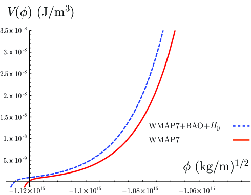
Figure 1: The phantom potential obtained from observational data fitting of WMAP7 and WMAP7+BAO+$H_{0}$.

Let us now consider the equation-of-state parameter for the phantom field, that is for the dark energy sector. As we mentioned in the end of section II, it is given by $w_{DE}(t)={p_{\phi}(t)}/{\rho_{\phi}(t)}$, with $p_{\phi}(t)$ and $\rho_{\phi}(t)$ given by relations (22) and (21) respectively. Finally, one can extract the redshift dependence using (23). One can therefore use WMAP7 and WMAP7+BAO+$H_{0}$ observational data in order to fit the evolution of $w_{DE}(z)$ at late times, that is for $t\rightarrow t_{s}$, or equivalently for $z\rightarrow-1$. For the WMAP7+BAO+$H_{0}$ combined dataset we find

$$w_{DE}(z) \approx \frac{1}{2}-\frac{6.068}{3.670-(1+z)^{3.307}},$$ (36)

while for the WMAP7 dataset alone we have

$$w_{DE}(z) \approx \frac{1}{2}-\frac{6.328}{3.824-(1+z)^{3.309}}.$$ (37)

As we observe, at $t\rightarrow t_{s}$, $w_{DE}$ becomes -1.153 for the combined dataset and -1.155 for the WMAP7 dataset alone. However, as we have already discussed in the end of section II, at $t\rightarrow t_{s}$ despite the finiteness of $w_{DE}$, the phantom dark energy density and pressure become infinite. These behaviors are the definition of a Big Rip BigRip2 , and this acts as a self-consistency test of our model.

V Conclusions

In this work we investigated phantom cosmology in which the scale factor is a power law. After constructing the scenario, we used observational data in order to impose constraints on the model parameters, focusing on the power-law exponent $\beta$ and on the Big Rip time $t_{s}$.

Using the WMAP7 dataset alone, we found that the power-law exponent is $\beta\approx-6.5\pm 0.4$ while the Big Rip is realized at $t_{s}\approx 102.3\pm 3.5$ Gyr, in 1$\sigma$ confidence level. Additionally, the dark-energy equation-of-state parameter $w_{DE}$ lies always below the phantom divide as expected, and at the Big Rip it remains finite and equal to -1.155. However, both the phantom dark-energy density and pressure diverge at the Big Rip.

Using WMAP7+BAO+$H_{0}$ combined observational data we found that $\beta\approx-6.51^{+0.24}_{-0.25}$, while $t_{s}\approx 104.5^{+1.9}_{-2.0}$ Gyr, in 1$\sigma$ confidence level. Moreover, $w_{DE}$ at the Big Rip becomes -1.153. Finally, in order to present a more transparent picture, we provided the reconstructed phantom potential.

In summary, we observe that phantom power-law cosmology can be compatible with observations, exhibiting additionally the usual phantom features, such is the future Big Rip singularity. However, it exhibits also the known disadvantage that the dark-energy equation-of-state parameter lies always below the phantom divide, by construction. In order to acquire a more realistic picture, describing also the phantom divide crossing, as it might be the case according to observations, one should proceed to the investigation of quintom power-law cosmology, considering apart from the phantom a canonical scalar field, too. Such a project is left for future investigation.

Finally, let us make a comment on the nature of the investigated scenarios. Although the classical behavior of phantom fields has a very rich phenomenology and can be compatible with observations, as it is known the discussion about the construction of quantum field theory of phantoms is still open in the literature. For instance in Cline:2003gs the authors reveal the causality and stability problems and the possible spontaneous breakdown of the vacuum into phantoms and conventional particles in four dimensions. However, on the other hand, there have also been serious attempts in overcoming these difficulties and construct a phantom theory consistent with the basic requirements of quantum field theory quantumphantom0 , with the phantom fields arising as an effective description. The present analysis is just a first approach on phantom power-law cosmology. Definitely, the subject of quantization of such scenarios is open and needs further investigation.

Appendix A Observational data and constraints

In this Appendix we briefly review the main sources of observational constraints used in this work, namely WMAP7 Cosmic Microwave Background (CMB), Baryon Acoustic Oscillations (BAO), and Observational Hubble Data ($H_{0}$). In our calculations we take the total likelihood $L\propto e^{-\chi^{2}/2}$ to be the product of the separate likelihoods of BAO, CMB and $H_{0}$. Thus, the total $\chi^{2}$ is

$$\chi^{2}(p_{s})=\chi^{2}_{CMB}+\chi^{2}_{BAO}+\chi^{2}_{H_{0}}.$$ (38)

a. CMB constraints

We use the CMB data to impose constraints on the parameter space, following the recipe described in Komatsu:2008hk . The “CMB shift parameters” Wang1 are defined as:

$$R\equiv\sqrt{\Omega_{m0}}H_{0}r\left(z_{*}\right),\,\quad l_{a}\equiv\pi r\left(z_{*}\right)/r_{s}\left(z_{*}\right).$$ (39)

$R$ can be physically interpreted as a scaled distance to recombination, and $l_{a}$ can be interpreted as the angular scale of the sound horizon at recombination. $r(z)$ is the comoving distance to redshift $z$ defined as

$$r(z)\equiv\int_{0}^{z}\frac{1}{H\left(z\right)}dz,$$ (40)

while $r_{s}\left(z_{*}\right)$ is the comoving sound horizon at decoupling (redshift $z_{*}$), given by

$$r_{s}\left(z_{*}\right)=\int_{z_{*}}^{\infty}\frac{1}{H\left(z\right)\sqrt{3\left(1+R_{b}/\left(1+z\right)\right)}}dz.$$ (41)

The quantity $R_{b}$ is the ratio of the energy density of photons to baryons, and its value can be calculated as $R_{b}=31500\Omega_{b0}h^{2}\left(T_{CMB}/2.7K\right)^{-4}$, ($\Omega_{b0}$ being the present day density parameter for baryons) using $T_{CMB}=2.725$ Komatsu:2008hk . The redshift at decoupling $z_{*}\left(\Omega_{b0},\Omega_{m0},h\right)$ can be calculated from the following fitting formula husugiyama :

$$z_{*}=1048\left[1+0.00124\left(\Omega_{b0}h^{2}\right)^{-0.738}\right]\left[1+g_{1}\left(\Omega_{m0}h^{2}\right)^{g_{2}}\right],$$ (42)

with $g_{1}$ and $g_{2}$ given by:

$$g_{1} = \frac{0.0783\left(\Omega_{b0}h^{2}\right)^{-0.238}}{1+39.5\left(\Omega_{b0}h^{2}\right)^{0.763}}$$

$$g_{2} = \frac{0.560}{1+21.1\left(\Omega_{b0}h^{2}\right)^{1.81}}.$$

Finally, the $\chi^{2}$ contribution of the CMB reads

$$\chi^{2}_{CMB}=\mathbf{V}_{\rm CMB}^{\mathbf{T}}\mathbf{C}_{\rm inv}\mathbf{V}_{\rm CMB}.$$ (43)

Here $\mathbf{V}_{\rm CMB}\equiv\mathbf{P}-\mathbf{P}_{\rm data}$, where $\mathbf{P}$ is the vector $\left(l_{a},R,z_{*}\right)$ and the vector $\mathbf{P}_{\rm data}$ is formed from the WMAP $5$-year maximum likelihood values of these quantities Komatsu:2008hk . The inverse covariance matrix $\mathbf{C}_{\rm inv}$ is also provided in Komatsu:2008hk .

b. Baryon Acoustic Oscillations constraints

In this case the measured quantity is the ratio $d_{z}=r_{s}\left(z_{d}\right)/D_{V}\left(z\right)$, where $D_{V}\left(z\right)$ is the so called “volume distance”, defined in terms of the angular diameter distance $D_{A}\equiv r\left(z\right)/\left(1+z\right)$ as

$$D_{v}\left(z\right)\equiv\left[\frac{\left(1+z\right)^{2}D_{A}^{2}(z)z}{H(z)}\right]^{1/3},$$ (44)

and $z_{d}$ is the redshift of the baryon drag epoch, which can be calculated from the fitting formula HuEisenstein :

$$z_{d}=\frac{1291\left(\Omega_{m0}h^{2}\right)^{0.251}}{1+\left(\Omega_{M0}h^{2}\right)^{0.828}}\left[1+b_{1}\left(\Omega_{b0}h^{2}\right)^{b_{2}}\right],$$ (45)

where $b_{1}$ and $b_{2}$ are given by

$$b_{1} = 0.313\left(\Omega_{m0}h^{2}\right)^{-0.419}\left[1+0.607\left(\Omega_{m0}h^{2}\right)^{0.674}\right]$$

$$b_{2} = 0.238\left(\Omega_{m0}h^{2}\right)^{0.223}.$$

We use the two measurements of $d_{z}$ at redshifts $z=0.2$ and $z=0.35$ Percival:2009xn . We calculate the $\chi^{2}$ contribution of the BAO measurements as:

$$\chi^{2}_{BAO}=\mathbf{V}_{\rm BAO}^{\mathbf{T}}\mathbf{C}_{\rm inv}\mathbf{V}_{\rm BAO}.$$ (46)

Here the vector $\mathbf{V}_{\rm BAO}\equiv\mathbf{P}-\mathbf{P}_{\rm data}$, with $\mathbf{P}\equiv\left(d_{0.2},d_{0.35}\right)$, and $\mathbf{P}_{\rm data}\equiv\left(0.1905,0.1097\right)$, the two measured BAO data points Percival:2009xn . The inverse covariance matrix is provided in Percival:2009xn .

c. Observational Hubble Data constraints

The observational Hubble data are based on differential ages of the galaxies ref:JL2002 . In ref:JVS2003 , Jimenez et al. obtained an independent estimate for the Hubble parameter using the method developed in ref:JL2002 , and used it to constrain the equation of state of dark energy. The Hubble parameter, depending on the differential ages as a function of the redshift $z$, can be written as

$$H(z)=-\frac{1}{1+z}\frac{dz}{dt}.$$ (47)

Therefore, once $dz/dt$ is known, $H(z)$ is directly obtained ref:SVJ2005 . By using the differential ages of passively-evolving galaxies from the Gemini Deep Deep Survey (GDDS) ref:GDDS and archival data ref:archive1 , Simon et al. obtained $H(z)$ in the range of $0\lesssim z\lesssim 1.8$ ref:SVJ2005 . We use the twelve observational Hubble data from ref:0905 listed in Table 3.

$z$	0	0.1	0.17	0.27	0.4	0.48	0.88	0.9	1.30	1.43	1.53	1.75
$H(z)\ ({\rm km~{}s^{-1}\,Mpc^{-1})}$	74.2	69	83	77	95	97	90	117	168	177	140	202
$1\sigma$ uncertainty	$\pm 3.6$	$\pm 12$	$\pm 8$	$\pm 14$	$\pm 17$	$\pm 60$	$\pm 40$	$\pm 23$	$\pm 17$	$\pm 18$	$\pm 14$	$\pm 40$

Table 3: The observational $H(z)$ data ref:0905 .

The best-fit values of the model parameters from observational Hubble data ref:SVJ2005 are determined by minimizing

$$\chi_{H_{0}}^{2}(p_{s})=\sum_{i=1}^{12}\frac{[H_{th}(p_{s};z_{i})-H_{obs}(z_{i})]^{2}}{\sigma^{2}(z_{i})},$$ (48)

where $p_{s}$ denotes the parameters contained in the model, $H_{th}$ is the predicted value for the Hubble parameter, $H_{obs}$ is the observed value, $\sigma(z_{i})$ is the standard deviation measurement uncertainty, and the summation runs over the $12$ observational Hubble data points at redshifts $z_{i}$.

References

- (1) A. G. Riess et al. [Supernova Search Team Collaboration], Astron. J. 116, 1009 (1998); S. Perlmutter et al. [Supernova Cosmology Project Collaboration], Astrophys. J. 517, 565 (1999); R. Amanullah et al., Astrophys. J. 716, 712 (2010) [arXiv:1004.1711 [astro-ph.CO]].
- (2) J. Dunkley et al. [WMAP Collaboration], Astrophys. J. Suppl. 180, 306 (2009) [arXiv:0803.0586 [astro-ph]]; E. Komatsu et al., arXiv:1001.4538 [astro-ph.CO]; D. Larson et al., arXiv:1001.4635 [astro-ph.CO].
- (3) M. Tegmark et al. [SDSS Collaboration], Phys. Rev. D 69, 103501 (2004).
- (4) S. W. Allen, et al., Mon. Not. Roy. Astron. Soc. 353, 457 (2004).
- (5) V. Sahni and A. Starobinsky, Int. J. Mod. Phy. D 9, 373 (2000); P. J. Peebles and B. Ratra, Rev. Mod. Phys. 75, 559 (2003).
- (6) P. J. Steinhardt, Critical Problems in Physics (1997), Princeton University Press.
- (7) J. Sola and H. Stefancic, Phys. Lett. B 624, 147 (2005); I. L. Shapiro and J. Sola, Phys. Lett. B 682, 105 (2009).
- (8) B. Ratra and P. J. E. Peebles, Phys. Rev. D 37, 3406 (1988); C. Wetterich, Nucl. Phys. B 302, 668 (1988); A. R. Liddle and R. J. Scherrer, Phys. Rev. D 59, 023509 (1999); I. Zlatev, L. M. Wang and P. J. Steinhardt, Phys. Rev. Lett. 82, 896 (1999); Z. K. Guo, N. Ohta and Y. Z. Zhang, Mod. Phys. Lett. A 22, 883 (2007); S. Dutta, E. N. Saridakis and R. J. Scherrer, Phys. Rev. D 79, 103005 (2009); E. N. Saridakis and S. V. Sushkov, Phys. Rev. D 81, 083510 (2010).
- (9) R. R. Caldwell, M. Kamionkowski and N. N. Weinberg, Phys. Rev. Lett. 91, 071301 (2003).
- (10) R. R. Caldwell, Phys. Lett. B 545, 23 (2002); S. Nojiri and S. D. Odintsov, Phys. Lett. B 562, 147 (2003); P. Singh, M. Sami and N. Dadhich, Phys. Rev. D 68, 023522 (2003); J. M. Cline, S. Jeon and G. D. Moore, Phys. Rev. D 70, 043543 (2004); V. K. Onemli and R. P. Woodard, Phys. Rev. D 70, 107301 (2004); W. Hu, Phys. Rev. D 71, 047301 (2005); M. R. Setare and E. N. Saridakis, JCAP 0903, 002 (2009); E. N. Saridakis, Nucl. Phys. B 819, 116 (2009); S. Dutta and R. J. Scherrer, Phys. Lett. B 676, 12 (2009).
- (11) B. Feng, X. L. Wang and X. M. Zhang, Phys. Lett. B 607, 35 (2005); E. Elizalde, S. Nojiri and S. D. Odintsov, Phys. Rev. D 70, 043539 (2004); Z. K. Guo, et al., Phys. Lett. B 608, 177 (2005); M.-Z Li, B. Feng, X.-M Zhang, JCAP, 0512, 002 (2005); B. Feng, M. Li, Y.-S. Piao and X. Zhang, Phys. Lett. B 634, 101 (2006); S. Capozziello, S. Nojiri and S. D. Odintsov, Phys. Lett. B 632, 597 (2006); W. Zhao and Y. Zhang, Phys. Rev. D 73, 123509 (2006); Y. F. Cai, T. Qiu, Y. S. Piao, M. Li and X. Zhang, JHEP 0710, 071 (2007); E. N. Saridakis and J. M. Weller, Phys. Rev. D 81, 123523 (2010); Y. F. Cai, T. Qiu, R. Brandenberger, Y. S. Piao and X. Zhang, JCAP 0803, 013 (2008); M. R. Setare and E. N. Saridakis, Phys. Lett. B 668, 177 (2008); M. R. Setare and E. N. Saridakis, Int. J. Mod. Phys. D 18, 549 (2009); Y. F. Cai, E. N. Saridakis, M. R. Setare and J. Q. Xia, Phys. Rept. 493 (2010) 1; T. Qiu, Mod. Phys. Lett. A 25, 909 (2010).
- (12) S. D. H. Hsu, Phys. Lett. B 594, 13 (2004); M. Li, Phys. Lett. B 603, 1 (2004); Q. G. Huang and M. Li, JCAP 0408, 013 (2004); M. Ito, Europhys. Lett. 71, 712 (2005); X. Zhang and F. Q. Wu, Phys. Rev. D 72, 043524 (2005); D. Pavon and W. Zimdahl, Phys. Lett. B 628, 206 (2005); S. Nojiri and S. D. Odintsov, Gen. Rel. Grav. 38, 1285 (2006); E. Elizalde, S. Nojiri, S. D. Odintsov and P. Wang, Phys. Rev. D 71, 103504 (2005); H. Li, Z. K. Guo and Y. Z. Zhang, Int. J. Mod. Phys. D 15, 869 (2006); E. N. Saridakis, Phys. Lett. B 660, 138 (2008); E. N. Saridakis, JCAP 0804, 020 (2008); E. N. Saridakis, Phys. Lett. B 661, 335 (2008).
- (13) P. Horava, Phys. Rev. D 79, 084008 (2009); G. Calcagni, JHEP 0909, 112 (2009); E. Kiritsis and G. Kofinas, Nucl. Phys. B 821, 467 (2009); H. Lu, J. Mei and C. N. Pope, Phys. Rev. Lett. 103, 091301 (2009); E. N. Saridakis, Eur. Phys. J. C 67, 229 (2010); X. Gao, Y. Wang, R. Brandenberger and A. Riotto, Phys. Rev. D 81, 083508 (2010); G. Leon and E. N. Saridakis, JCAP 0911, 006 (2009); M. i. Park, JHEP 0909, 123 (2009); S. Dutta and E. N. Saridakis, JCAP 1001, 013 (2010); C. Germani, A. Kehagias and K. Sfetsos, JHEP 0909, 060 (2009); C. Bogdanos and E. N. Saridakis, Class. Quant. Grav. 27, 075005 (2010); E. Kiritsis, Phys. Rev. D 81, 044009 (2010); D. Capasso and A. P. Polychronakos, JHEP 1002, 068 (2010); S. Dutta and E. N. Saridakis, JCAP 1005, 013 (2010); G. Koutsoumbas and P. Pasipoularides, arXiv:1006.3199 [hep-th]; M. Eune and W. Kim, arXiv:1007.1824 [hep-th].
- (14) R. Kallosh, J. Kratochvil, A. Linde, E. Linder and M. Shmakova, JCAP 0310, 015 (2003); P. F. Gonzalez-Diaz, Phys. Rev. D 68, 021303 (2003).
- (15) S. Nojiri, S. D. Odintsov and S. Tsujikawa, Phys. Rev. D 71, 063004 (2005).
- (16) M. Sami and A. Toporensky, Mod. Phys. Lett. A 19, 1509 (2004); Y. S. Piao and Y. Z. Zhang, Phys. Rev. D 70, 063513 (2004); P. F. Gonzalez-Diaz and J. A. Jimenez-Madrid, Phys. Lett. B 596, 16 (2004); P. Wu and H. W. Yu, JCAP 0605, 008 (2006); Y. S. Piao, Phys. Rev. D 78, 023518 (2008); E. Elizalde, S. Nojiri, S. D. Odintsov, D. Saez-Gomez and V. Faraoni, Phys. Rev. D 77, 106005 (2008). C. J. Feng, X. Z. Li and E. N. Saridakis, Phys. Rev. D 82, 023526 (2010).
- (17) S. Nojiri and S. D. Odintsov, Gen. Rel. Grav. 38, 1285 (2006). I. P. Neupane and H. Trowland, arXiv:0902.1532 [gr-qc]; I. P. Neupane and C. Scherer, JCAP 0805, 009 (2008).
- (18) E. W. Kolb, Astrophys. J. 344, 543 (1989).
- (19) P. J. E. Peebles, Principles of physical cosmology, Princeton, USA: Univ. Pr. (1993).
- (20) M. Sethi, A. Batra and D. Lohiya, Phys. Rev. D 60, 108301 (1999); M. Kaplinghat, G. Steigman and T. P. Walker, Phys. Rev. D 61, 103507 (2000).
- (21) M. Kaplinghat, G. Steigman, I. Tkachev and T. P. Walker, Phys. Rev. D 59, 043514 (1999).
- (22) D. Lohiya and M. Sethi, Class. Quan. Grav. 16, 1545 (1999).
- (23) G. Sethi, A. Dev and D. Jain, Phys. Lett. B 624, 135 (2005).
- (24) A. Dev, D. Jain and D. Lohiya, arXiv:0804.3491 [astro-ph].
- (25) S. W. Allen, R. W. Schmidt, A. C. Fabian, Mon. Not. Roy. Astro. Soc. 334, L11 (2002); S. W. Allen, R. W. Schmidt, A. C. Fabian, H. Ebeling, Mon. Not. Roy. Astro. Soc. 342, 287 (2003); S. W. Allen, R. W. Schmidt, H. Ebeling, A. C. Fabian and L. van Speybroeck, Mon. Not. Roy. Astro. Soc. 353 457 (2004).
- (26) Z. H. Zhu, M. Hu, J. S. Alcaniz and Y. X. Liu, Astron. and Astrophys. 483, 15 (2008).
- (27) A. Dev, M. Safonova, D. Jain and D. Lohiya, Phys. Lett. B 548, 12 (2002).
- (28) J. S. Alcaniz, A. Dev and D. Jain, Astrophys. J. 627, 26 (2005).
- (29) S. Nojiri, S. D. Odintsov and M. Sasaki, Phys. Rev. D 71, 123509 (2005).
- (30) S. Das, P. S. Corasaniti and J. Khoury, Phys. Rev. D 73, 083509 (2006); M. Kaplinghat and A. Rajaraman, Phys. Rev. D 75, 103504 (2007).
- (31) F. Briscese, E. Elizalde, S. Nojiri and S. D. Odintsov, Phys. Lett. B 646, 105 (2007).
- (32) D. Larson et al., arXiv:1001.4635 [astro-ph.CO].
- (33) W. J. Percival et al., Mon. Not. Roy. Astron. Soc. 401, 2148 (2010).
- (34) A. G. Riess et al., Astrophys. J. 699, 539 (2009); D. Stern et al., JCAP 1002, 008 (2010).
- (35) E. Komatsu et al. [WMAP Collaboration], Astrophys. J. Suppl. 180, 330 (2009).
- (36) M. Hicken et al., Astrophys. J. 700, 1097 (2009).
- (37) M. Kowalski et al. [Supernova Cosmology Project Collaboration], Astrophys. J. 686, 749 (2008).
- (38) R. Kessler et al., Astrophys. J. Suppl. 185, 32 (2009).
- (39) E. Komatsu et al., arXiv:1001.4538 [astro-ph.CO].
- (40) G. R. Bengochea, arXiv:1010.4014 [astro-ph.CO].
- (41) R. G. Vishwakarma and J. V. Narlikar, arXiv:1010.5272 [astro-ph.CO].
- (42) K. Thepsuriya and B. Gumjudpai, arXiv:0904.2743 [astro-ph.CO].
- (43) B. Gumjudpai, JCAP 0809, 028 (2008).
- (44) J. M. Cline, S. Jeon and G. D. Moore, Phys. Rev. D 70, 043543 (2004).
- (45) S. Nojiri and S. D. Odintsov, Phys. Lett. B 562, 147 (2003); S. Nojiri and S. D. Odintsov, Phys. Lett. B 571, 1 (2003).
- (46) Y. Wang and P. Mukherjee, Astrophys. J. 650, 1 (2006).
- (47) W. Hu and N. Sugiyama, Astrophys. J. 471, 542 (1996).
- (48) D. J. Eisenstein and W. Hu, Astrophys. J. 496, 605 (1998).
- (49) R. Jimenez and A. Loeb, Astrophys. J. 573 37 (2002).
- (50) R. Jimenez, L. Verde, T. Treu and D. Stern, Astrophys. J. 593 622 (2003).
- (51) J. Simon, L. Verde and R. Jimenez, Phys. Rev. D 71 123001 (2005).
- (52) R. G. Abraham et al., Astron. J. 127 2455 (2004).
- (53) J. Dunlop et al., Nature 381 581 (1996); H. Spinrad et al., Astrophys. J. 484 581 (1997); T. Treu et al., Mon. Not. Roy. Astron. Soc. 308 1037 (1999); T. Treu et al., Mon. Not. Roy. Astron. Soc. 326 221 (2001); T. Treu et al., Astrophys. J. Lett. 564 L13 (2002); L. A. Nolan, J. S. Dunlop, R. Jimenez and A. F. Heavens, Mon. Not. Roy. Astron. Soc. 341 464 (2003).