Interface solitons in one-dimensional locally-coupled lattice systems

Abstract

Fundamental solitons pinned to the interface between two discrete lattices coupled at a single site are investigated. Serially and parallel-coupled identical chains (System 1 and System 2), with the self-attractive on-site cubic nonlinearity, are considered in one dimension. In these two systems, which can be readily implemented as arrays of nonlinear optical waveguides, symmetric, antisymmetric and asymmetric solitons are investigated by means of the variational approximation (VA) and numerical methods. The VA demonstrates that the antisymmetric solitons exist in the entire parameter space, while the symmetric and asymmetric modes can be found below some critical value of the coupling parameter. Numerical results confirm these predictions for the symmetric and asymmetric fundamental modes. The existence region of numerically found antisymmetric solitons is also limited by a certain value of the coupling parameter. The symmetric solitons are destabilized via a supercritical symmetry-breaking pitchfork bifurcation, which gives rise to stable asymmetric solitons, in both systems. The antisymmetric fundamental solitons, which may be stable or not, do not undergo any bifurcation. In bistability regions stable antisymmetric solitons coexist with either symmetric or asymmetric ones.

I Introduction

The study of surface modes in multi-layered optical media has begun long ago early . Recently, a great deal of attention was attracted to studies of solitons pinned to interfaces between different nonlinear optical media, at least one of which carries a lattice structure. Such surface solitons were predicted theoretically in diverse settings surface-theory and soon after that created in experiments surface-experiment . Surface solitons were also considered in the general context of junctions between different discrete lattices 3 . In these studies, it was concluded that the self-trapped surface modes acquire novel properties, different from those of the solitons known in uniform lattices. In particular, discrete surface states can only exist above a certain threshold value of the total power (the soliton’s norm), and a bistability is possible, with different surface modes coexisting at a common value of the power.

Generally speaking, these nonlinear modes may be considered as a variety of optical solitons pinned by defects, which were also studied theoretically defect-theory ; molinakivshar and experimentally defect-experiment ; Roberto in many systems, continual and discrete (a comprehensive review of the topic of discrete and lattice solitons in optics, including the interaction with defects, was given in recent articles big-review ; for a general review of discrete solitons, see book PGK ). These studies have demonstrated that discrete nonlinear photonic systems may support spatially localized states with different symmetries, which can be controlled by the insertion of suitable defects into the lattice molinakivshar . Localized modes supported by defects of optical lattices (OLs) were also studied in models of Bose-Einstein condensates (BECs) Konotop .

Another topic which is relevant to the present work is the possibility of the spontaneous symmetry breaking (SSB) in two-mode symmetric settings with a linear coupling between two subsystems. An alternative realization of settings which give rise to the SSB is represented by double-well potentials (in that case, the two coupled modes correspond to states trapped in the two symmetric wells). A specific version of the SSB corresponds to the double-well pseudopotential, induced by a symmetric spatial modulation of the local nonlinearity coefficient Dong .

SSB bifurcations, which destabilize symmetric states and give rise to asymmetric ones, were originally predicted in terms of the self-trapping in discrete systems Scott . In the physically important model of dual-core nonlinear fibers, the SSB instability was discovered in Ref. Wright , and the respective bifurcations for continuous-wave states were studied in detail in Ref. Snyder , for various types of the intra-core nonlinearities. It is also relevant to mention early work earlier , which put forward the SSB concept in the framework of the nonlinear Schrödinger (NLS) equation. Further, the SSB was studied in detail for solitons in the model of the dual-core fiber with the cubic (Kerr) nonlinearity Akhmediev ; malomed . Similar analysis was later performed for gap solitons in the models of dual-core Mak and tri-core gubeskys1 fiber Bragg gratings, and for matter-wave solitons in the BEC loaded into a dual-core potential trap combined with a longitudinal OL. The latter analysis was performed in the models with both one 1D-BEC and two 2D-BEC longitudinal dimensions (1D and 2D, respectively).

The limit case of a very strong OL corresponds to a discrete lattice wannier . In that case, the SSB of 1D and 2D discrete solitons in the system of two linearly coupled discrete NLS equations (DNLSEs) was investigated in Ref. VA .

In addition to the studies of the SSB in diverse two-core systems with the cubic nonlinear terms, this effect was also analyzed in models describing optical media with quadratic chi2 and cubic-quintic CQ nonlinearities. In the latter case, the SSB diagrams feature loops, with asymmetric solitons existing at intermediate values of the total power, while only symmetric modes can be found at low and high powers.

General conclusions about the character of the SSB in solitons can be drawn from the above-mentioned works. The self-focusing nonlinearity induces the SSB of symmetric modes, with a trend to make the respective bifurcation subcritical, whose characteristic feature is a bistability region, in which stable symmetric and asymmetric solitons coexist. The self-focusing nonlinearity does not induce any bifurcation of antisymmetric solitons. In the absence of the periodic potential induced by the OL, the entire family of the antisymmetric solitons is unstable.

However, if the self-attractive nonlinearity acts in the combination with a sufficiently strong OL, the antisymmetric solitons may be stable. In the same case, the SSB bifurcation is transformed from subcritical into the supercritical one, which does not admit the coexistence of stable symmetric and asymmetric solitons. Nevertheless, a global bistability of a different type takes place in this situation, as stable antisymmetric solitons coexist with their symmetric and asymmetric counterparts, below and above the bifurcation point, respectively (in the 2D setting, both families of the asymmetric and antisymmetric solitons attain a termination point at high values of the total power, due to the onset of the collapse driven by the self-attraction).

On the other hand, in the models combining the self-defocusing nonlinearity and OL potentials, symmetric solitons do not suffer any SSB, while antisymmetric solitons are destabilized by the anti-symmetry-breaking pitchfork bifurcation, which is always of the supercritical type.

In this work we aim to study localized modes at the interface of two 1D uniform discrete lattices (chains) with the cubic onsite nonlinearity, which are linearly coupled either in series (System 1, see Fig. 1 below) or in parallel (System 2, see Fig. 4). In fact, the former configuration may be realized as a single discrete lattice with a spring defect, in the form of a locally modified inter-site coupling constant (such a system has been actually created in optics, as an array of nonlinear waveguides with a modified separation between two of them Roberto ). System 2 differs from that introduced in Ref. VA by the fact that the two uniform identical chains placed in parallel planes are linearly coupled in the transverse direction at a singe site, rather than featuring the uniform linear coupling. Analyzing localized defect/surface modes in these two systems, we focus on their symmetry properties – in particular, with the intention to investigate SSB transitions in them.

The presentation is organized as follows. The systems, 1 and 2, are introduced in Section 2, where we consider the existence and stability of various localized modes, applying the variational approximation (VA) and the Vakhitov-Kolokolov (VK) stability criterion. Dynamical properties of the discrete solitons with different symmetries are investigated by means of numerical methods, including the computation of the linear-stability eigenvalues and direct simulations in Section 4. The paper is concluded by Section 5.

II Fundamental surface solitons in the system of two coupled lattices

II.1 System 1: the serial coupling

The system formed by two linked identical semi-infinite chains is displayed in Fig. 1, with inter-site coupling constant $C$ inside the chains, and constant $\varepsilon$ accounting for the linkage between them. We consider only the case when $C$ and $\varepsilon$ have the same sign, as opposite signs of the inter-site couplings are difficult to realize in optical and BEC systems. The on-site nonlinearity is cubic, with the respective coefficient, $\gamma$, being constant throughout the system. Thus, this model is described by the following DNLSE system,

$$i\frac{d\phi_{n}}{dz}+\phi_{n+1}+\phi_{n-1}+\left|\phi_{n}\right|^{2}\phi_{n} = 0,\ n\neq 0,1,$$

$$i\frac{d\phi_{0}}{dz}+\varepsilon\phi_{1}+\phi_{-1}+\left|\phi_{0}\right|^{2}\phi_{0} = 0,$$

$$i\frac{d\phi_{1}}{dz}+\varepsilon\phi_{0}+\phi_{2}+\left|\phi_{1}\right|^{2}\phi_{1} = 0,$$ (1)

where $z$ is the propagation distance (assuming that the chains correspond to two semi-infinite arrays of parallel optical waveguides), and an obvious rescaling is used to fix $C=\gamma=1$ [that is, $\varepsilon$ which figures in Eqs. (1) is $\varepsilon/C$, in terms of Fig. 1].

This system may be considered as the usual DNLSE containing a local ”spring defect”. As mentioned above, such a system has been created in optics, in the form of a regular array of parallel waveguiding cores, with a change of the distance between two of them Roberto . The interaction of lattice solitons with this array defect was studied experimentally in Ref. Roberto .

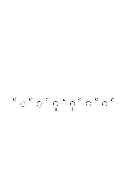
Figure 1: A schematic of System 1, which consists of two semi-infinite identical chains, linked by the modified linear coupling $\varepsilon$ between sites $n=0$ and $n=1$.

Stationary solutions for solitons formed at the interface between the chains are looked for as usual, $\phi_{n}=u_{n}\exp\left(i\mu z\right)$, where $u_{n}$ and $\mu$ are real lattice field and propagation constant. The corresponding stationary equations following from Eqs. (1) are

$$-\mu u_{n}+u_{n+1}+u_{n-1}+u_{n}^{3} = 0,\ n\neq 0,1,$$

$$-\mu u_{0}+\varepsilon u_{1}+u_{-1}+u_{0}^{3} = 0,$$

$$-\mu u_{1}+\varepsilon u_{0}+u_{2}+u_{1}^{3} = 0.$$ (2)

II.1.1 The variational approximation

Equations (2) can be derived from the Lagrangian,

$$L=L_{-}+L_{+}+2\varepsilon u_{0}u_{1},$$ (3)

$$L_{-} \equiv \sum_{n=-\infty}^{-1}\left(-\mu u_{n}^{2}+\frac{1}{2}u_{n}^{4}+2u_{n}u_{n+1}\right)+\left(-\mu u_{0}^{2}+\frac{1}{2}u_{0}^{4}\right),~{}$$

$$L_{+} \equiv \sum_{n=1}^{\infty}\left(-\mu u_{n}^{2}+\frac{1}{2}u_{n}^{4}+2u_{n}u_{n+1}\right),$$

where $L_{\pm}$ are the intrinsic Lagrangians of the two semi-infinite chains, and the last term in Eq. (3) accounts for the coupling between them. To apply the variational approximation (VA), we follow Ref. VA and adopt an ansatz consisting of two parts:

$$u_{n} = A\exp{(an)},\ \mathrm{for}\ n\leq 0,$$

$$u_{n} = B\exp{(-a(n-1))},\ \mathrm{for}\ n\geq 1.$$ (4)

This ansatz admits different amplitudes, $A\neq B$, of the solution in the linked chains, but postulates a common width of the ansatz in both of them, $a^{-1}$. Actually, the SSB is represented by the appearance of asymmetric solutions, with $A^{2}\neq B^{2}$.

Amplitudes $A$ and $\,B$ are treated below as variational parameters. As concerns inverse width $a$, it is fixed through a solution of the linearization of Eqs. (2) at $|n|\rightarrow\infty$,

$$a=\ln\left(\mu/2+\sqrt{\mu^{2}/4-1}\right),$$ (5)

which implies that the propagation constant takes values $\mu>2$. Relation (5) may also be represented in the following forms, that will be used below:

$$s\equiv e^{-a}=\frac{\mu}{2}-\sqrt{\frac{\mu^{2}}{4}-1},~{}\mu=s+s^{-1}.$$ (6)

The substitution of ansatz (4) into Eq. (3) yields the corresponding effective Lagrangian, where Eq. (5) is used to eliminate $\mu$ in favor of $s$:

$$L_{\mathrm{eff}}=\left(L_{-}\right)_{\mathrm{eff}}+\left(L_{+}\right)_{\mathrm{eff}}+2\varepsilon AB,$$ (7)

$$\left(L_{-}\right)_{\mathrm{eff}} = -s^{-1}A^{2}+\frac{1}{2\left(1-s^{4}\right)}A^{4}$$

$$\left(L_{+}\right)_{\mathrm{eff}} = -s^{-1}B^{2}+\frac{1}{2\left(1-s^{4}\right)}B^{4}.$$ (8)

This Lagrangian gives rise to the Euler-Lagrange equations for amplitudes $A$ and $B$: $\left(\partial/\partial A\right)\left(L_{-}\right)_{\mathrm{eff}}+2\varepsilon B=0,\left(\partial/\partial B\right)\left(L_{+}\right)_{\mathrm{eff}}+2\varepsilon A=0$, or, in the explicit form,

$$-s^{-1}A+\frac{1}{1-s^{4}}A^{3}+\varepsilon B = 0$$

$$-s^{-1}B+\frac{1}{1-s^{4}}B^{3}+\varepsilon A = 0.$$ (9)

These equations allow us to predict the existence of three different species of the localized modes: symmetric ones, with $A=B$, antisymmetric with $A=-B$, and asymmetric with $A^{2}\neq B^{2}$.

The results of the VA are reported below, along with the respective numerical results. It will be seen that the VA predicts characteristics of the symmetric and asymmetric modes very accurately, while the approximation is essentially less accurate for the antisymmetric solitons.

II.1.2 Existence regions for the interface solitons

The solution for the symmetric solitons (SyS) is easily obtained from Eqs. (9),

$$A^{2}=({1-s^{4}})(s^{-1}-\varepsilon).$$ (10)

The dependence of this amplitude on $\varepsilon$ for fixed $s=\left(5-\sqrt{21}\right)/2\approx\allowbreak 0.21$, which corresponds to $\mu=5$, is plotted in Fig. 2. As follows from Eq. (10), in System 1 the existence domain of the SyS solutions at a given value of the propagation constant, $\mu$, is limited to $\varepsilon<$$\varepsilon_{e}^{(1)}$$\equiv s^{-1}$. The upper existence limit for the SyS is seen in Fig. 2, and also in Fig. 3(a), which shows the existence regions predicted by the VA for all the types of the solitons in the plane of $\left(\varepsilon,\mu\right)$, along with the numerically found counterparts of these regions (the procedure of obtaining numerical results is described below).

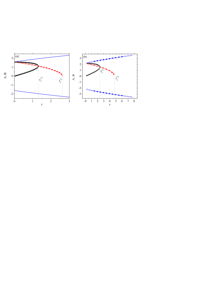
Figure 2: (Color online) Amplitudes $A$ and $B$ of asymmetric, symmetric, and antisymmetric solitons (black, red, and blue colors, respectively), as predicted by the VA (lines) and obtained in the numerical form (AS - circles, SyS - triangles, AnS - squares), versus $\varepsilon$, for System 1, at fixed values of the propagation constant: $\mu=3$ (a) and $\mu=5$ (b). The dotted green vertical lines denote the critical values of $\varepsilon$ limiting the existence regions of the asymmetric ($\varepsilon_{c}$) and symmetric ($\varepsilon_{e}$) solitons. For $\mu=3$, antisymmetric solitons were not found in the numerical form. Empty and full symbols pertain to unstable and stable solitons, respectively, as concluded from the numerical investigation.

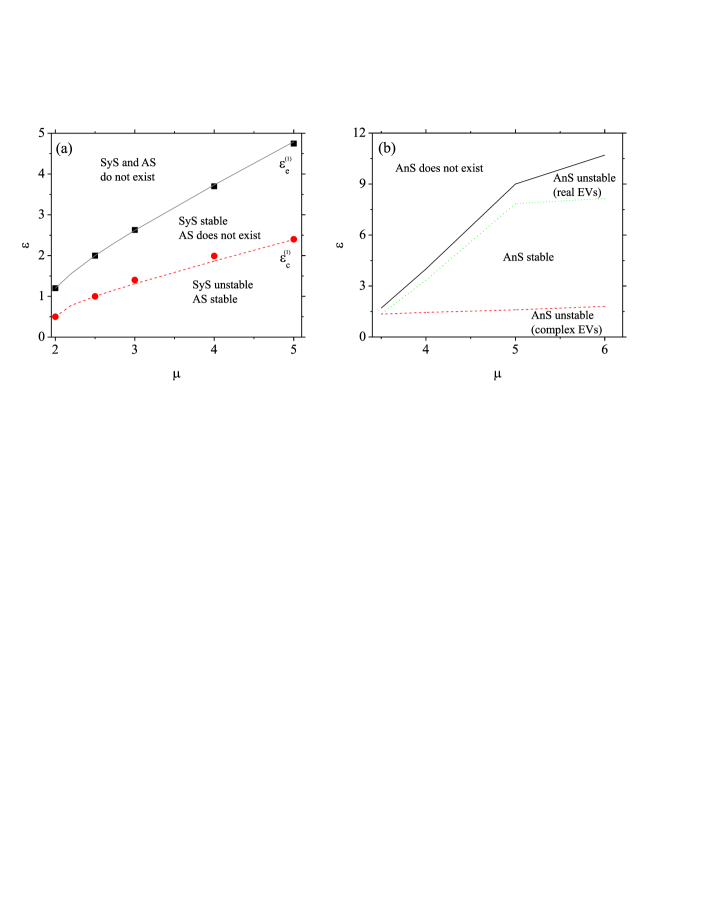
Figure 3: (Color online) (a) The existence and stability diagrams for the fundamental symmetric (SyS) and asymmetric (AS) solitons in System 1, generated by means of the VA (curves) and numerical computations (symbols), in the plane of $\left(\varepsilon,\mu\right)$. Black squares, which mark the boundary of the SyS existence region, are located very close to the respective line $\varepsilon_{e}^{(1)}(\mu)$ predicted by the VA (see Fig. 2). Red circles, which denote the numerically found boundary of the AS existence region, are also close to the VA-predicted curve $\varepsilon_{c}^{(1)}(\mu)$, along which the symmetry-breaking bifurcation takes place, destabilizing the SyS and giving birth to two mutually symmetric branches of the AS modes. (b) The existence and stability borders for the antisymmetric mode (AnS) in the same parameter plane, found in the numerical form only (the variational approximation does not predict existence limits for the AnS). Inside the instability areas in (b), the type of the respective unstable eigenvalues (EVs) of small perturbations is indicated.

The existence range of the asymmetric solution (AS), with $A^{2}\neq B^{2}$, can be estimated by taking the difference of two equations (9) and canceling a common factor $\left(A-B\right)$:

$$\left(s^{-1}+\varepsilon\right)=A^{2}+B^{2}+AB.$$ (11)

In the limit of $A-B\rightarrow 0$, Eq. (11) yields the following relation:

$$A^{2}=(1/3)({1-s^{4}})\left(s^{-1}-\varepsilon\right).$$ (12)

Equating expressions (10) and (12), one can predict the value of the linkage constant at which the SSB bifurcation gives birth to the pair of AS in System 1,

$${\varepsilon}_{c}^{(1)}=\left(2s\right)^{-1}.$$ (13)

For broad solitons, with $a\rightarrow\infty$, i.e., $s\rightarrow 1$ [see Eq. (4)], $\varepsilon$${}_{c}^{(1)}$ given by Eq. (13) approaches a limit value, $\varepsilon$${}_{c}^{(1)}=1/2$, while for strongly localized solitons, with $\mu\rightarrow\infty$ and $s<<1$, relation (6) demonstrates that Eq. (13) yields $\varepsilon$${}_{c}^{(1)}\approx\mu/2$, cf. Figs. 2 and 3).

The general solution for the AS can be found after some algebraic manipulations with Eqs. (9) (replacing the equations by their sum and difference, and solving the latter equations for $A^{2}+B^{2}$ and $AB$, cf. similar exact solutions obtained for the SSB in the double-well pseudopotential in Ref. Dong ):

$$A = \frac{\varepsilon\sqrt{2s({1-s^{4}})}}{\sqrt{1+\sqrt{1-4s^{2}{\varepsilon}^{2}}}},$$

$$B = \sqrt{\frac{{1-s^{4}}}{2s}}\sqrt{1+\sqrt{1-4s^{2}{\varepsilon}^{2}}}.$$ (14)

This solution exists at ${\varepsilon<\varepsilon}_{c}$, where ${\varepsilon}_{c}$ is precisely the bifurcation value given by Eq. (13). The conclusion that the asymmetric modes exist when the coupling constant  ($\varepsilon$) is not too large is very natural Akhmediev -2D-BEC , VA . Indeed, the extreme case of the asymmetric solution, with $A\neq 0$ and $B=0$, is obviously possible in the limit of $\varepsilon=0$. Equally natural is the conclusion that the symmetric mode is stable at ${\varepsilon>\varepsilon}_{c}$ and unstable at ${\varepsilon<\varepsilon}_{c}$, while the asymmetric mode is stable in the entire region of its existence, as seen in Fig. 2. Finally, we notice that the SSB bifurcations observed in Fig. 2 (and in Fig. 5 below, which pertains to System 2) are clearly the pitchfork bifurcations of the supercritical type, on the contrary to the subcritical bifurcation reported in Ref. VA for the model based on two uniformly coupled parallel chains.

For antisymmetric solitons (AnS) the amplitude is obtained from Eq. (9) by substituting $A=-B$, which yields

$$A^{2}=\left({1-s^{4}}\right)\left(s^{-1}+\varepsilon\right).$$ (15)

Relation (15) is plotted versus $\varepsilon$ for fixed $\mu=5$ by blue lines in Fig. 2. As follows from this relation, the VA predicts the existence of the AnS in the entire parameter space, on the contrary to the limited existence regions predicted for the SyS and AS modes. However, numerical results reported below demonstrate that the AnS also have their existence limits, see Fig. 3(b).

II.1.3 Stability

The stability of the discrete solitons predicted by the VA can be first estimated by dint of the VK criterion, $dP/d\mu>0$, where $P\equiv\sum_{n=-\infty}^{n=+\infty}u_{n}^{2}$ is the total power (norm) of the soliton isrl . Being necessary, but not the sufficient, this condition should be combined with the spectral criterion, which requires all the eigenvalues of small perturbations around the solitons to be stable.

The power corresponding to ansatz (4) is

$$P=\left(1-s^{2}\right)^{-1}({A^{2}}+B^{2}).$$ (16)

For the SyS solution with $A=B,$ Eqs. (16) and (10) yield $P=2(1+s^{2})\left(s^{-1}-\varepsilon\right)$. This expression satisfies condition $\partial P/\partial s<0$, which is tantamount to the VK criterion, at all values of $\varepsilon$.  Nevertheless, it is obvious that the the branch of the symmetric solitons is destabilized by the SSB bifurcation, hence it is unstable at $\varepsilon<\varepsilon_{c}$, as shown in Fig. 2 (it is well known that the respective instability is not detected by the VK criterion Akhmediev -2D-BEC , VA ).

For the AS solutions, the substitution of Eq. (14) into Eq. (16) produces a simple expression for the total power, which does not depend on $\varepsilon$:

$$P=\left(1+s^{2}\right)/s.$$ (17)

It also satisfies the VK criterion in the entire region of the existence of the asymmetric interface modes.

Finally, for the antisymmetric modes in System 1, with $A=-B$, the use of Eq. (15) gives $P=2(1+s^{2})\left(s^{-1}+\varepsilon\right)$. In this case, condition $dP/ds<0$ is satisfied only at

$$\varepsilon>{\varepsilon}_{s}^{(1)}=\left(1-s^{2}\right)s^{-3},$$ (18)

while the antisymmetric modes are VK-unstable in the other part of their existence region, at $\varepsilon<\varepsilon_{s}$. This is in contrast with the above conclusions that the symmetric and asymmetric solitons comply with the VK criterion in their entire existence domains.

II.1.4 Comparison to the uniform chain

It is instructive to compare the results predicted for System 1 by the VA to the well-known properties of the uniform infinite chain described by the usual DNLSE, which corresponds to Eqs. (1) with $\varepsilon=1$ PGK . To this end, one may consider cuts of Figs. 2(a) and (b) through $\varepsilon=1$. Along these cuts, one finds an unstable SyS, stable AS, and stable AnS. In terms of the infinite uniform chain, the SyS corresponds to an inter-site-centered (alias off-site) discrete soliton, which is, indeed, always unstable in the usual DNLSE PGK . The fact that the spring defect with $\varepsilon>1$ makes the off-site soliton stable beyond the bifurcation point, i.e., at $\varepsilon<\varepsilon_{c}$, is remarkable by itself.

Further, what we define as the AS, corresponds to the usual on-site-centered soliton in the ordinary DNLSE, which is always stable, as is well known. And finally, the AnS soliton is tantamount to the localized twisted mode in the DNLSE setting twisted , which is stable with small amplitudes and unstable if its amplitude is larger, as in the case corresponding to Fig. 2(b) at $\varepsilon=1$.

II.2 System 2: the parallel coupling

The system formed by two identical infinite uniform chains, coupled by the transverse link at the single site, is shown in Fig. 4.

Figure 4: The schematic of System 2, which is built of two uniform identical chains placed in parallel planes, which are linearly coupled in the transverse direction at site n = 0. The longitudinal and transverse coupling constants are C and $\varepsilon$, respectively.

The corresponding DNLSE system is (where, as well as in Eqs. (1), we set $C=\gamma=1$, by means of rescaling):

$$i\frac{d\phi_{n}}{dz}+\phi_{n+1}+\phi_{n-1}\gamma\left|\phi_{n}\right|^{2}\phi_{n} = 0,\ n\neq 0,$$

$$i\frac{d\phi_{0}}{dz}+\phi_{1}+\phi_{-1}+\varepsilon\psi_{0}+\left|\phi_{0}\right|^{2}\phi_{0} = 0,$$

$$i\frac{d\psi_{n}}{dz}+\psi_{n+1}+\psi_{n-1}+\left|\psi_{n}\right|^{2}\psi_{n} = 0,\ n\neq 0,$$

$$i\frac{d\psi_{0}}{dz}+\psi_{1}+\psi_{-1}+\varepsilon\phi_{0}+\gamma\left|\psi_{0}\right|^{2}\psi_{0} = 0.$$ (19)

The stationary solutions are looked for in the form of $\phi_{n}=u_{n}\exp\left(i\mu z\right)$ and $\psi_{n}=v_{n}\exp\left(i\mu z\right),$ with a common propagation constant, $\mu$, and real functions $u_{n}$ and $v_{n}$ satisfying the following equations:

$$-\mu u_{n}+u_{n+1}+u_{n-1}+\left|u_{n}\right|^{2}u_{n} = 0;\ n\neq 0$$

$$-\mu v_{n}+v_{n+1}+v_{n-1}+\left|v_{n}\right|^{2}v_{n} = 0;\ n\neq 0$$

$$-\mu u_{0}+u_{1}+u_{-1}+\varepsilon v_{0}+\left|u_{0}\right|^{2}u_{0} = 0;$$

$$-\mu v_{0}+v_{1}+v_{-1}+\varepsilon u_{0}+\left|v_{0}\right|^{2}v_{0} = 0.$$ (20)

II.2.1 The variational approximation

The stationary equations can be derived from the Lagrangian, $L=L_{1}+L_{2}+2\varepsilon u_{0}v_{0},$where $L_{1}$ and $L_{2}$ are the intrinsic Lagrangians of the two uniform chains. Similar to System 1, the VA is based on the exponentially localized ansatz with possibly different amplitudes $A$ and $B$ but a common width, $a^{-1}$, cf. Eqs. (4):

$$u_{n}=A\exp{(-a|n|),~{}}v_{n}=B\exp{(-a|n|)}.$$ (21)

By substituting this ansatz into the Lagrangian, and using, as above, Eq. (6) to eliminate $\mu$, we obtain

$$L_{\mathrm{eff}}=-\frac{1-s^{2}}{s}\left(A^{2}+B^{2}\right)+\frac{1}{2}\frac{1+s^{4}}{1-s^{4}}\left(A^{4}+B^{4}\right)+2\varepsilon AB,$$ (22)

cf. Eqs. (7) and (8). Finally, the Euler-Lagrange equations, $\partial L_{\mathrm{eff}}/\partial A=\partial L_{\mathrm{eff}}/\partial B=0$, applied to Lagrangian (22), take the following form:

$$-\frac{1-s^{2}}{s}A+\frac{1+s^{4}}{1-s^{4}}A^{3}+\varepsilon B = 0$$

$$-\frac{1-s^{2}}{s}B+\frac{1+s^{4}}{1-s^{4}}B^{3}+\varepsilon A = 0.$$ (23)

II.2.2 Existence regions for soliton solutions

The solution for the SyS (symmetric soliton), with $A=B$, is immediately obtained from Eq. (23):

$$A^{2}=\frac{1-s^{4}}{1+s^{4}}\left(\frac{1-s^{2}}{s}-\varepsilon\right).$$ (24)

This relation is plotted in Fig. 5 for $\mu=5$. Similar to the case of System 1, it follows from Eq. (24) that in System 2 the SyS exists at $\varepsilon<$$\varepsilon_{e}^{(2)}$$=\left(1-s^{2}\right)/s$, as shown in Figs. 5 and 6. In the latter figure, the critical value $\varepsilon_{e}^{(2)}$ is plotted by the black line.

The existence range of the AS solutions can be determined by means of the same procedure which was used above in the case of System 1. The result is that, in the present case, the asymmetric modes exist at

$$\varepsilon<{\varepsilon}_{c}^{(2)}=\left(1-s^{2}\right)/\left(2s\right),$$ (25)

cf. Eq. (13). For the broad asymmetric solitons $(s\rightarrow 1)$, $\varepsilon_{c}^{(2)}$ approaches the limiting value $\varepsilon_{c}^{(2)}$$=0$, while for the strongly localized solitons $(s<<1)$ we obtain $\varepsilon$${}_{c}\approx\mu/2$. The full solution for the AS mode can be found too, cf. Eq. (14) for System 1:

$$A = \sqrt{\frac{{1-s^{4}}}{2s(1+s^{4})}}\sqrt{\left(1-s^{2}\right)+\sqrt{(1-s^{2})^{2}-4s^{2}{\varepsilon}^{2}}}$$

$$B = \varepsilon\sqrt{\frac{2s(1-s^{4})}{1+s^{4}}}\frac{1}{\sqrt{{1-s}^{2}+\sqrt{(1-s^{2})^{2}-4s^{2}{\varepsilon}^{2}}}}$$ (26)

Note that the AS solution exists at $\varepsilon<\left(1-s^{2}\right)/\left(2s\right)$, which is exactly equivalent to Eq. (25), obtained above by means of a different algebra. The amplitudes of AS at the interface sites are plotted in Fig. 5.

The solution for the antisymmetric $(A=-B)$ solitons (AnS) produced by Eqs. (23) is

$$A^{2}=\frac{1-s^{4}}{1+s^{4}}\left(\frac{1-s^{2}}{s}+\varepsilon\right).$$ (27)

As seen from here, the AnS are predicted by the VA to exist in the entire parameter space.

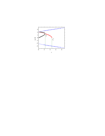
Figure 5: (Color online) The same as in Fig. 2(b) (i.e., with $\mu=5$), but for System 2.

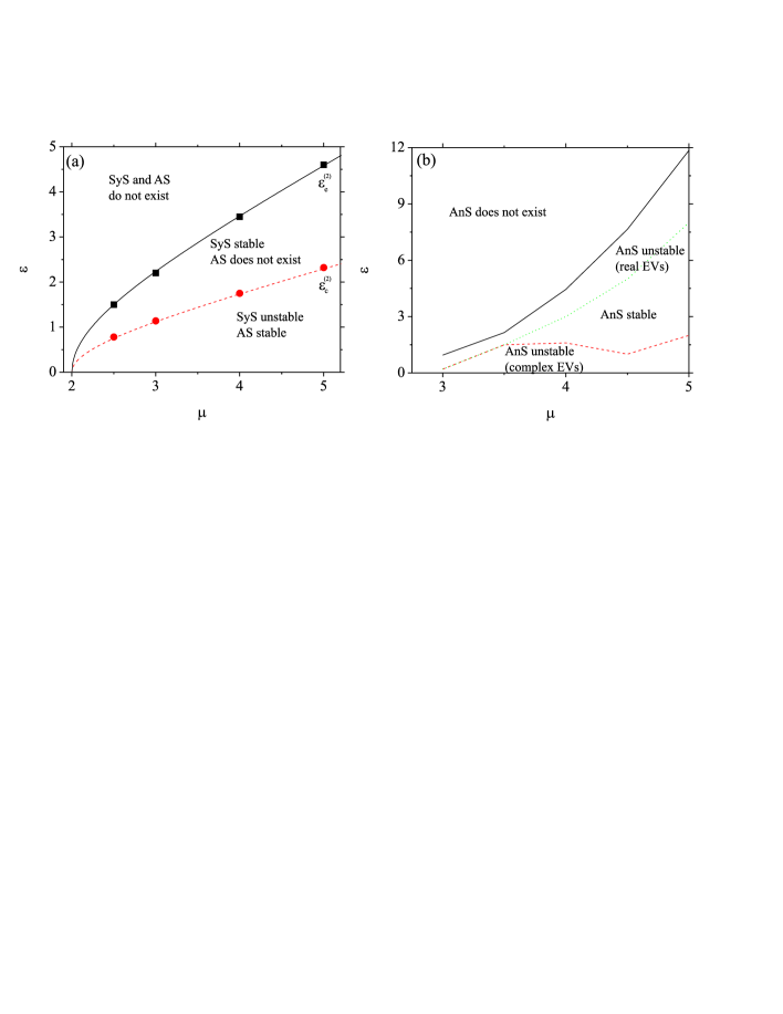
Figure 6: (Color online) The same as in Fig. 3, but for System 2.

II.2.3 Stability

The VK criterion may also be applied to the soliton solutions predicted in System 2. The total power of the solutions based on ansatz (21) is

$$P=\frac{1+s^{2}}{1-s^{2}}({A^{2}}+B^{2}).$$ (28)

For the SyS solution (24) with $A=B$, Eq. (28) yields

$$P=\frac{2(1+s^{2})^{2}}{1+s^{4}}\left(\frac{1-s^{2}}{s}-\varepsilon\right),$$ (29)

which satisfies the VK condition, $\partial P/\partial s<0$ (tantamount to $\partial P/\partial\mu>0$) in the entire existence region. For the AS solution given by Eq. (26), the calculation of norm (28) yields a result which does not depend on $\varepsilon,$ cf. Eq. (17) for the AS solution in System 1:

$$P=\frac{(1+s^{2})(1-s^{4})}{s(1+s^{4})},$$ (30)

whose VK slope, $\partial P/\partial\mu$, is again positive in the entire region where this solution exists.

Lastly, for the AnS solution, with $A=-B,$ the power (29) is

$$P=\frac{2(1+s^{2})^{2}}{1+s^{4}}\left(\frac{1-s^{2}}{s}+\varepsilon\right),$$ (31)

whose slope may change its sign. The eventual conclusion is that the AnS solution satisfies the VK criterion only in a part of its existence region, viz., at

$$\varepsilon>{\varepsilon}_{s}^{(2)}=\frac{1+s^{2}}{4s^{3}(1-s^{2})}-\frac{1-s^{2}}{s},$$ (32)

cf. similar result (18) obtained above for the AnS solutions in System 1.

III Numerical results

To verify the predictions of the VA, we numerically solved stationary equations (2) and (20) for both models, applying the relaxation method and an algorithm based on the modified Powell minimization method nashi . The initial guess used to construct fundamental solitons centered at the interface of the linked semi-infinite chains which constitute System 1 (Fig. 1) was taken as $U_{0}$ $=U_{1}=A>0$ for SyS solutions, $U_{0}$ $=A>0,\,U_{1}=B>0$ for AS solutions, and $U_{0}=A>0,U_{1}=-A$ for ones of the AnS type, with the VA-predicted values of $A$ and $B$, while in initial values of the lattice field are set to be zero at all other sites.

The initial ansatz for the parallel-coupled lattices which constitute System 2 (Fig. 4) was $U_{0}$ $=V_{0}$ $=A>0$ for SyS modes, $U_{0}$ $=A>0,\,V_{0}$ $=B>0$ for AS modes, $U_{0}$ $=A>0,V_{0}$ $=-A$ for modes of the AnS type, and $U_{n}=V_{n}=0$ at all other sites. The results presented here are obtained for identical coupled chains with $N_{1}=N_{2}=50$ or $N_{1}=N_{2}=51$ sites, for Systems 1 and 2, respectively. In other words, the total number of sites is $N=100$ in System 1, and $N=102$ in System 2, which features the parallel chains. The link between the chains in System 1 was set between the sites with indexes $n=0$ and $n=1$, and in System 2 the transverse coupling between the parallel lattices was introduced at $n=0$.

The stability of the stationary modes was first checked by dint of the linear-stability analysis, i.e., the calculation of eigenvalues (EVs) for modes of small perturbations, following the lines of Refs. nashi . The respective calculations were performed in parameter space ($\varepsilon$, $\mu$). Then, the results were verified in direct numerical simulations of full equations, (1) and (19). The simulations were based on a numerical code which used the sixth-order Runge-Kutta algorithm, as in Ref. nashi . The simulations were initialized by taking the stationary soliton profiles, to which random perturbations were added.

Typical shapes of symmetric, asymmetric and antisymmetric solitons found in the numerical form are displayed in Fig. 7 for System 1 and in Fig. 8 for System 2. In the same figures, the numerical shapes are compared with those obtained by means of the VA. The respective dependencies of the solitons’ amplitudes $A$ and $B$ on parameter $\varepsilon$, which accounts for the linkage between the two chains, are displayed for all the soliton species, alongside their VA-predicted counterparts, in the above figures 2 and 3. Further, the numerical results demonstrate that all the species of the solitons, including the AnS, exist in bounded regions of the parameter space, as shown in the above figures 3 and 6, for Systems 1 and 2, respectively.

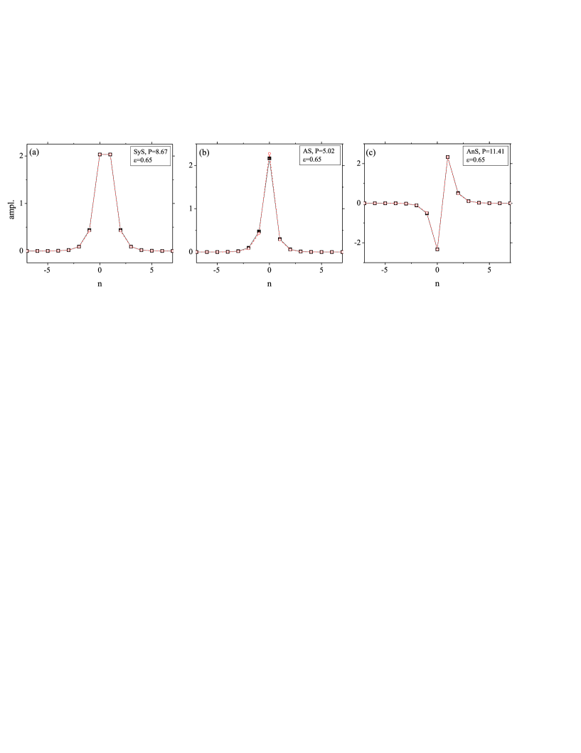
Figure 7: Profiles of the fundamental solitons (interface modes) in System 1: (a) symmetric (SyS), (b) asymmetric (AS), and (c) antisymmetric (AnS). The inter-chain linkage strength is $\varepsilon=0.65$. The total powers corresponding to each mode are indicated in the panels. Black solid lines with squares denote numerically generated solitons, while red dashed lines with circles denote variationally obtained solitons.

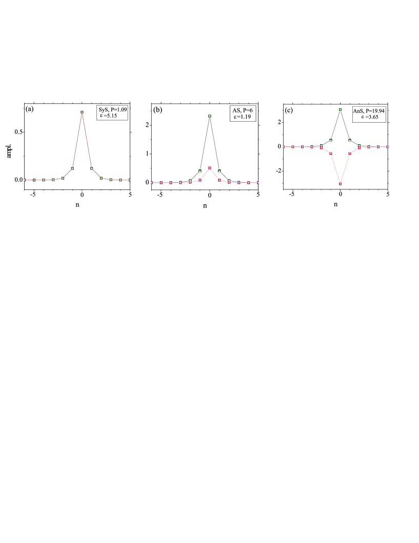
Figure 8: (Color online) Profiles of fundamental solitons in System 2 (two parallel lattices, L₁ and L₂, coupled by the transverse link with strength $\varepsilon$), obtained for $\mu=6$. The values of $\varepsilon$ and the total powers are indicated in the panels. Black solid and red dashed lines show the profiles in lattices L₁ and L₂ obtained numerically. The corresponding soliton profiles predicted by the VA are denoted by hollow squares (green for L₁ and blue for L₂). (a) A symmetric (SyS) soliton, (b) an asymmetric (AS) soliton, and (c) an antisymmetric (AnS) soliton.

The comparison with the numerical results demonstrates that the predictions of the VA for the symmetric and asymmetric discrete solitons are very accurate. However, the VA fails to predict the existence borders for the antisymmetric modes. A reason for the latter problem may be that the strong interaction force at the interface, in the case of the opposite signs of the lattice fields at adjacent sites, see Figs. 7(c) and 8(c), makes the simple form of the VA adopted above inaccurate.

In the instability region, the SyS solutions are characterized by the EV spectrum consisting of real pairs. Under small asymmetric perturbations, an unstable SyS sheds off a part of its total power and relaxes into an asymmetric breather with a smaller power, as shown for System 1 in Fig. 9 (a). As in other conservative systems, Akhmediev -2D-BEC , VA , the asymmetric breathers cannot readily self-trap into stationary solitons. In System 2, the behavior of the unstable symmetric solitons is quite similar.

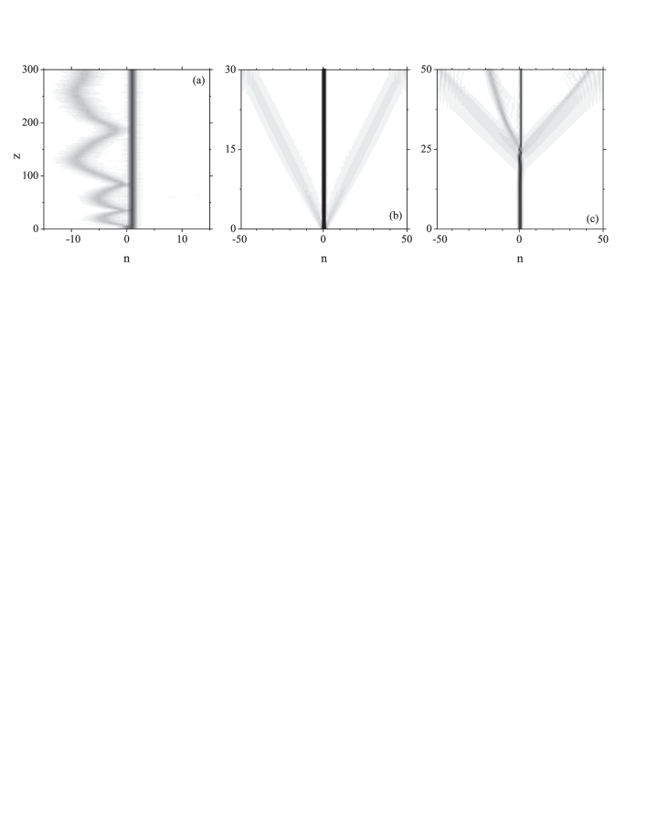
Figure 9: Typical examples of the evolution of perturbed unstable solitons in System 1. (a) A symmetric soliton, with $\varepsilon=0.65,\,\mu=6.425$. Other panels display antisymmetric solitons, with $\mu=6$: (b) $\varepsilon=9.1$ (real unstable EVs, see Fig. 5), and (c) $\varepsilon=1.15$ (complex EVs). The unstable symmetric soliton, after shedding off a part of its power, evolves into an asymmetric breather. The unstable antisymmetric solitons transform into breathers too, see the text.

In both Systems 1 and 2, the EV spectra for the stationary asymmetric modes are stable in the entire existence region. This is also confirmed by direct simulations, which show that perturbed AS develop small-amplitude persistent oscillations without any trend to destruction.

The antisymmetric solitons change their stability twice, in both configurations considered, 1 and 2. With the decrease of $\varepsilon$ at fixed $\mu$, the unstable AnS branch, which is characterized by a pair of real EVs [in the area between the green dotted and black solid lines in Figs. 3 (b) and 6 (b)], changes into the stable one. With the further decrease of $\varepsilon,$ the AnS loses its stability through the appearance of two pairs (a quartet) of complex EVs with significant real parts [in the area below the red dashed line in Figs. 3 (b) and 6 (b)]. For example, the antisymmetric modes corresponding to $\mu=5$ acquire the oscillatory instability, with the decrease of $\varepsilon$, at $\varepsilon\approx 1.5$ and $2$ in Systems 1 and 2, respectively, which is indicated by the appearance of a quartet of complex EVs in their spectra (in the areas below the red line in Figs 3 and 6). Note that the VA has also shown that the AnS change their stability according to the VK criterion, see Eqs. (18) and (32). However, the corresponding VA-predicted critical curves, $\varepsilon_{c}^{(1,2)}(\mu)$, are found to be situated beyond the numerically obtained existence regions of the AnS solutions.

The predictions concerning the stability of the AnS were checked by direct simulations. In Fig. 9(b) and (c), the evolution of typical unstable antisymmetric modes in System 1 is displayed. Panels (b) and (c) in this figure illustrate the evolution of the unstable AnS whose EV spectrum contains a pair of real EVs, or a complex EV quartet, respectively. The unstable antisymmetric modes radiate away a part of their power, relaxing to antisymmetric (b) or asymmetric (c) interface modes, which exhibit small-amplitude persistent oscillations. In System 2, the same happens with the unstable AnS belonging to the instability area below the red (dashed) line in Fig. 6. However, in contrast to that, the AnS in System 2 which is characterized by the EV spectrum with a pair of real EVs turn out to be robust under the action of small perturbations. They do not emit radiation waves, staying localized and strongly pinned to the link connecting the two infinite chains.

Returning to the global existence diagrams, it is worthy to note that two bistability areas can be identified in both systems, 1 and 2: the domain of the coexistence of stable symmetric and antisymmetric solitons, or the one featuring the simultaneous stability of asymmetric and antisymmetric modes, on the opposite sides on the SSB bifurcation. This result is in accordance with similar findings reported in other linearly-coupled two-component systems featuring the self-focusing nonlinearity 1D-BEC ; 2D-BEC .

IV Conclusion

In this paper, we have investigated several species of fundamental localized modes formed at the interface between two linearly coupled lattices (chains) with the cubic on-site nonlinearity. Two configurations were considered: the one with the linkage between two semi-infinite chains (in other words, the usual discrete NLS model with a spring defect), and two infinite chains placed in parallel planes which are coupled by the transverse link at one site. These systems can be readily implemented as arrays of optical waveguides.

In both models, the VA (variational approximation) was used to predict the existence regions, in the parameter space of $(\mu,\varepsilon)$ (the propagation constant and the strength of the coupling between the two subsystems), for the localized symmetric, asymmetric and antisymmetric discrete solitons pinned to the interface. The stability of the modes was predicted as per the VK criterion and general properties of the supercritical pitchfork bifurcation, which destabilizes the SyS (symmetric solitons) giving birth to AS (asymmetric solitons). The predictions were verified against numerical results, as concerns the existence and stability of all the soliton species. In both systems considered, the existence regions of all the localized modes are bounded. The AS are stable in their entire existence domain. The existence and stability domains for AnS (antisymmetric solitons) were found in the numerical form. Both systems give rise to the bistability between the AnS on the one hand, and either SyS or AS, on the other. Direct simulations demonstrate that unstable SyS are transformed into asymmetric breathers. Those antisymmetric modes which are unstable shed off a part of the total power and also evolve into breathers. In System 2, in a part of the parametric domain where the computation of the eigenvalues predicts the instability of the antisymmetric localized modes, they actually evolve into strongly pinned robust spikes.

- (1) P. Yeh, A. Yariv, and A. Y. Cho, Appl. Phys. Lett. 32, 104 (1978); W. J. Tomlinson, Opt. Lett. 5, 323 (1980).
- (2) K. G. Makris, S. Suntsov, D. N. Christodoulides, G. I. Stegeman, and A. Hache, Opt. Lett. 30, 2466 (2005); M. I. Molina, R. A. Vicencio, and Y. S. Kivshar, ibid. 31, 1693 (2006); Y. V. Kartashov and L. Torner, ibid. 31, 2172 (2006); Y. V. Kartashov, V. A. Vysloukh, D. Mihalache, and L. Torner, ibid. 31, 2329 (2006); M. I. Molina, I. L. Garanovich, A. A. Sukhorukov, and Y. S. Kivshar, ibid. 31, 2332 (2006); K. G. Makris, J. Hudock, D. N. Christodoulides, G. I. Stegeman, O. Manela, and M. Segev, ibid. 31, 2774 (2006); Y. V. Kartashov, V. A. Vysloukh, and L. Torner, Phys. Rev. Lett. 96, 073901 (2006); Y. V. Kartashov, A. A. Egorov, V. A. Vysloukh, and L. Torner, Opt. Exp. 14, 4049 (2006); D. Mihalache, D. Mazilu, F. Lederer, and Y. S. Kivshar, Opt. Exp. 15, 589 (2007).
- (3) S. Suntsov, K. G. Makris, D. N. Christodoulides, G. I. Stegeman, A. Hache, R. Morandotti, H. Yang, G. Salamo, and M. Sorel, Phys. Rev. Lett. 96, 063901 (2006); E. Smirnov , M. Stepić, C. E. Ruter, D. Kip, V. Shandarov, Opt. Lett. 15, 2338 (2006); G. A. Siviloglou, K. G. Makris, R. Iwanow, R. Schiek, D. N. Christodoulides, G. I. Stegeman, Y. Min, and W. Sohler, Opt. Exp. 14, 5508 (2006); X. S. Wang, A. Bezryadina, Z. G. Chen, K. G. Makris, D. N. Christodoulides, and G. I. Stegeman, Phys. Rev. Lett. 98, 123903 (2007); A. Szameit, Y. V. Kartashov, F. Dreisow, T. Pertsch, S. Nolte, A. Tünnermann, and L. Torner, ibid. 98, 173903 (2007).
- (4) Yu. S. Kivshar, F. Zhang, and S. Takeno, Physica D 113, 248 (1998).
- (5) X. D. Cao and B. A. Malomed, , Phys. Lett. A 206, 177 (1995); W. Królikowski and Y. S. Kivshar, J. Opt. Soc. Am. B 13, 876 (1996); R. H. Goodman, R. E. Slusher, and M. I. Weinstein, ibid. 19, 1635 (2002); W. C. K. Mak, B. A. Malomed, and P. L. Chu, ibid. 20, 725 (2003); H. Susanto, G. Kevrekidis, B. A. Malomed, R. Carretero-González, and D. J. Frantzeskakis, Phys. Rev. E 75, 056605 (2007); F. Palmero, R. Carretero-González, J. Cuevas, P. G. Kevrekidis, and W. Królikowski, ibid. E 77, 036614 (2008)Q. E. Hoq, R. Carretero-González, P. G. Kevrekidis, B. A. Malomed, D. J. Frantzeskakis, Yu. V. Bludov, and V. V. Konotop, ibid. E 78, 036605 (2008).
- (6) Yu. S. Kivshar and M. I. Molina, Wave Motion 45, 59 (2007); M. I. Molina, and Yu. S. Kivshar, Opt. Lett. 33, 917 (2008).
- (7) U. Peschel, R. Morandotti, J. S. Aitchison, H. S. Eisenberg, and Y. Silberberg, Appl. Phys. Lett. 75, 1348 (1999); R. Morandotti, H. S. Eisenberg, D. Mandelik, Y. Silberberg, D. Modotto, M. Sorel, C. R. Stanley, and J. S. Aitchison, Opt. Lett. 28, 834 (2003); F. Fedele, J. K. Yang, and Z. G. Chen, ibid. 30, 1506 (2005); I. Makasyuk, Z. G. Chen, and J. K. Yang, Phys. Rev. Lett. 96, 223903 (2006); T. Schwartz, G. Bartal, S. Fishman, and M. Segev, Nature 446, 52 (2007).
- (8) R. Morandotti, H. S. Eisenberg, D. Mandelik, Y. Silberberg, D. Modotto, M. Sorel, C. R. Stanley, and J. S. Aitchison, Opt. Lett. 28, 834 (2003).
- (9) F. Lederer, G. I. Stegeman, D. N. Christodoulides, G. Assanto, M. Segev, and Y. Silberberg, Phys. Rep. 363, 1 (2008); Y. V. Kartashov, V. A. Vysloukh, and L. Torner,Progress in Optics 52, 63 (2009).
- (10) P. G. Kevrekidis, editor, The Discrete Nonlinear Schrödinger Equation: Mathematical Analysis, Numerical Computations, and Physical Perspectives (Springer: Berlin and Heidelberg, 2009).
- (11) V. A. Brazhnyi and V. V. Konotop, Mod. Phys. Lett. B 18, 627 (2004).
- (12) T. Mayteevarunyoo, B. A. Malomed, and G. Dong, Phys. Rev. A 78, 053601 (2008).
- (13) J. C. Eilbeck, P. S. Lomdahl, and A. C. Scott, Physica D 16, 318 (1985).
- (14) E. M. Wright, G. I. Stegeman, and S. Wabnitz, Phys. Rev. A 40, 4455 (1989).
- (15) A. W. Snyder, D. J. Mitchell, L. Poladian, D. R. Rowland, and Y. Chen, J. Opt. Soc. Am. B 8, 2102 (1991).
- (16) E. B. Davies, Comm. Math. Phys. 64, 191 (1979).
- (17) N. Akhmediev, and A. Ankiewicz, Phys. Rev. Lett. 70, 2395 (1993); P. L. Chu, B. A. Malomed, and G. D. Peng,J. Opt. Soc. A B 10, 1379 (1993); J. M. Soto-Crespo, and N. Akhmediev, Phys. Rev. E 48, 4710 (1993).
- (18) B. A. Malomed, I. Skinner, P. L. Chu, and G. D. Peng, Phys. Rev. E 53, 4084 (1996).
- (19) W. C. K. Mak, B. A. Malomed, and P. L. Chu,J. Opt. Soc. Am. B 15, 1685 (1998).
- (20) A. Gubeskys, and B. A. Malomed, Eur. Phys. J. D 28, 283 (2004).
- (21) A. Gubeskys, and B. A. Malomed, Physical Review A 75, 063602 (2007); M. Matuszewski, B. A. Malomed, and M. Trippenbach, Phys. Rev. A 75, 063621 (2007); M. Trippenbach, E. Infeld, J. Gocalek, M. Matuszewski, M. Oberthaler, and B. A. Malomed, Physical Review A 78, 013603 (2008).
- (22) A. Gubeskys and B. A. Malomed, Phys. Rev. A 76, 043623 (2007).
- (23) G. L. Alfimov, P. G. Kevrekidis, V. V. Konotop, and M. Salerno, Phys. Rev. E 66, 046608 (2002).
- (24) G. Herring, P. G. Kevrekidis, B. A. Malomed, R. Carretero-González, and D. J. Frantzeskakis, Physical Review E 76, 066606 (2007).
- (25) W. C. K. Mak, B.A. Malomed, and P. L. Chu, Phys. Rev. E 55, 6134 (1997); ibid. E 57, 1092 (1998).
- (26) R. Driben, B. A Malomed1 and P. L. Chu, J. Phys. B: At. Mol. Opt. Phys. 39, 2455 (2006); L. Albuch and B. A. Malomed, , Math. Comp. Simul. 74, 312 (2007); Z. Birnbaum and B. A. Malomed, Physica D 237, 3252 (2008).
- (27) B. A. Malomed and M. I. Weinstein,Phys. Lett. A 220, 91 (1996); Y. Sivan, B. Ilan, and G. Fibich, Phys. Rev. E 78, 046602, (2008).
- (28) E. W. Laedke, O. Kluth and K. H. Spatschek, Phys. Rev. E 54, 4299 (1996); M. Johansson and S. Aubry, Nonlinearity 10, 1151 (1997); S. Darmanyan and A. Kobyakov, and F. Lederer, Zh. Eksp. Teor. Fiz. 113, 1253 (1998) [J. Exp. Theor. Phys. 86, 682 (1998)]; P. G. Kevrekidis, A. R. Bishop, and K. Ø. Rasmussen, Phys. Rev. E 63, 036603 (2001); A. A. Sukhorukov and Y. S. Kivshar, , ibid. 65, 036609 (2002); A. Maluckov, M. Stepić, D. Kip, and L. Hadžievski, Eur. Phys. J. B 45, 539 (2005).
- (29) G. Gligorić, A. Maluckov, Lj. Hadžievski, and B. A. Malomed, Phys. Rev. A 79, 053609, (2009); G. Gligorić, A. Maluckov, Lj. Hadžievski, and B. A. Malomed, Phys. Rev. A 78, 063615, (2008).