Separable covariance arrays via the Tucker product, with applications to multivariate relational data

Abstract

Modern datasets are often in the form of matrices or arrays, potentially having correlations along each set of data indices. For example, data involving repeated measurements of several variables over time may exhibit temporal correlation as well as correlation among the variables. A possible model for matrix-valued data is the class of matrix normal distributions, which is parametrized by two covariance matrices, one for each index set of the data. In this article we describe an extension of the matrix normal model to accommodate multidimensional data arrays, or tensors. We generate a class of array normal distributions by applying a group of multilinear transformations to an array of independent standard normal random variables. The covariance structures of the resulting class take the form of outer products of dimension-specific covariance matrices. We derive some properties of these covariance structures and the corresponding array normal distributions, discuss maximum likelihood and Bayesian estimation of covariance parameters and illustrate the model in an analysis of multivariate longitudinal network data.

Some key words: Gaussian, matrix normal, multiway data, network, tensor, Tucker decomposition.

1 Introduction

This article provides a construction of and estimation for a class of covariance models and Gaussian probability distributions for array data consisting of multi-indexed values $\mbox{\bf{Y}}=\{y_{i_{1}},\ldots,y_{i_{K}}:i_{k}\in\{1,\ldots,m_{k}\},k=1,\ldots,K\}$. Such data have become common in many scientific disciplines, including the social and biological sciences. Researchers often gather relational data measured on pairs of units, where the population of units may consist of people, genes, websites or some other set of objects. Data on a single relational variable is often represented by a “sociomatrix” $\mbox{\boldmath{${\rm Y}$}}=\{y_{i,j},i\in\{1,\ldots,m\},j\in\{1,\ldots,m\},i\neq j\}$, a square matrix with an undefined diagonal, where $y_{i,j}$ represents the relationship between nodes $i$ and $j$.

Multivariate relational data include multiple relational measurements on the same node set, possibly gathered under different conditions or at different time points. Such data can be represented as a multiway array. For example, in this article we will analyze data on trade of several commodity classes between a set of countries over several years. These data can be represented as a four-way array $\mbox{\bf{Y}}=\{y_{i,j,k,t}\}$, where $y_{i,j,k,t}$ records the volume of exports of commodity $k$ from country $i$ to country $j$ in year $t$. For such data it is often of interest to identify similarities or correlations among data corresponding to the objects of a given index set. For example, one may want to identify nodes of a network that behave similarly across levels of the other factors of the array. For temporal datasets it may be important to describe correlations among data from adjacent time points. In general, it may be desirable to estimate or account for dependencies along each index set of the array.

For matrix valued data, such considerations have led to the use of separable covariance estimates, whereby the covariance of a population of matrices is estimated as being ${\rm Cov}[{\rm vec}(\mbox{\bf{Y}})]=\mathbf{\Sigma}_{2}\otimes\mathbf{\Sigma}_{1}$. In this parameterization $\mathbf{\Sigma}_{1}$ and $\mathbf{\Sigma}_{2}$ represent covariances among the rows and columns of the matrices, respectively. Such a covariance model may provide a stable and parsimonious alternative to an unrestricted estimate of ${\rm Cov}[{\rm vec}(\mbox{\bf{Y}})]$, the latter being unstable or even unavailable if the dimensions of the sample data matrices are large compared to the sample size. The family of matrix normal distributions with separable covariance matrices is studied in Dawid (1981), and an iterative algorithm for maximum likelihood estimation is given by Dutilleul (1999). Testing various hypotheses regarding the separability of the covariance structure, or the form of the component matrices, is considered in Lu and Zimmerman (2005); Roy and Khattree (2005); Mitchell et al. (2006) among others. Beyond the matrix-variate case, Galecki (1994) considers a separable covariance model for three-way arrays, but where the component matrices are assumed to have compound symmetry or an autoregressive structure.

In this article we show that the class of separable covariance models for random arrays of arbitrary dimension can be generated with a type of multilinear transformation known as the Tucker product (Tucker, 1964; Kolda, 2006). Just as a zero-mean multivariate normal vector with a given covariance matrix can be represented as a linear transformation of a vector of independent, standard normal entries, in Section 2 we show that a normal array with separable covariance structure can be represented by a multilinear transformation of an array of independent, standard normal entries. As a result, the calculations involved in obtaining maximum likelihood and Bayesian estimates are made simple via some basic tools of multilinear algebra. In Section 3 we adapt the iterative algorithm of Dutilleul (1999) to the array normal model, and provide a conjugate prior distribution and posterior approximation algorithm for Bayesian inference. Section 4 presents an example data analysis of trade volume data between pairs of 30 countries in 6 commodity types over 10 years. A discussion of model extensions and directions for further research follows in Section 5.

2 Separable covariance via array-matrix multiplication

2.1 Array notation and basic operations

An array of order $K$, or $K$-array, is a map from the product space of $K$ index sets to the real numbers. The different index sets are referred to as the modes of the array. The dimension vector of an array gives the number of elements in each index set. For example, for a positive integer $m_{1}$, a vector in $\mathbb{R}^{m_{1}}$ is a one-array with dimension $m_{1}$. A matrix in $\mathbb{R}^{m_{1}\times m_{2}}$ is a two-array with dimension $(m_{1},m_{2})$. A $K$-array Z with dimension $(m_{1},\ldots,m_{K})$ has elements $\{z_{i_{1},\ldots,i_{K}}:i_{k}\in\{1,\ldots,m_{k}\},k=1,\ldots,K\}$.

Array unfolding refers to the representation of an array by an array of lower order via combinations of various index sets of an array. A useful unfolding is the $k$-mode matrix unfolding, or $k$-mode matricization (De Lathauwer et al., 2000), in which a $K$-array Z is reshaped to form a matrix $\mbox{\bf{Z}}_{(k)}$ with $m_{k}$ rows and $\prod_{j:j\neq k}m_{k}$ columns. Each column corresponds to the entries of Z in which the $k$th index $i_{k}$ varies from 1 to $m_{k}$ and the remaining indices are fixed. The assignment of the remaining indices $\{i_{j}:j\neq k\}$ to columns of $\mbox{\bf{Z}}_{(k)}$ is determined by the following ordering on index sets: Letting $\mbox{\boldmath{${\rm i}$}}=(i_{1},\ldots,i_{K})$ and $\mbox{\boldmath{${\rm j}$}}=(j_{1},\ldots,j_{K})$ be two sets of indices, we say $\mbox{\boldmath{${\rm i}$}}<\mbox{\boldmath{${\rm j}$}}$ if $i_{k}<j_{k}$ for some $k$ and $i_{l}\leq j_{l}$ for all $l>k$. In terms of ordering the columns of the matricization, this means that the index corresponding to a lower-numbered mode “moves faster” than that of a higher-numbered mode.

De Lathauwer et al. (2000) define an array-matrix product via the usual matrix product as applied to matricizations. The $k$-mode product of an $m_{1}\times\cdots\times m_{K}$ array Z and a $n\times m_{k}$ matrix ${\rm A}$ is obtained by forming the $m_{1}\times\cdots\times m_{k-1}\times n\times m_{k+1}\times\cdots\times m_{K}$ array from the inversion of the $k$-mode matricization operation on the matrix $\mbox{\boldmath{${\rm A}$}}\mbox{\bf{Z}}_{(k)}$. The resulting array is denoted by $\mbox{\bf{Z}}\times_{k}\mbox{\boldmath{${\rm A}$}}$. Letting ${\rm F}$ and ${\rm G}$ be matrices of the appropriate sizes, important properties of this product include the following:

• $(\mbox{\bf{Z}}\times_{j}\mbox{\boldmath{${\rm F}$}})\times_{k}\mbox{\boldmath{${\rm G}$}}=(\mbox{\bf{Z}}\times_{k}\mbox{\boldmath{${\rm G}$}})\times_{j}\mbox{\boldmath{${\rm F}$}}=\mbox{\bf{Z}}\times_{j}\mbox{\boldmath{${\rm F}$}}\times_{k}\mbox{\boldmath{${\rm G}$}}$

• $(\mbox{\bf{Z}}\times_{j}\mbox{\boldmath{${\rm F}$}})\times_{j}\mbox{\boldmath{${\rm G}$}}=\mbox{\bf{Z}}\times_{j}(\mbox{\boldmath{${\rm G}$}}\mbox{\boldmath{${\rm F}$}})$

• $\mbox{\bf{Z}}\times_{j}(\mbox{\boldmath{${\rm F}$}}+\mbox{\boldmath{${\rm G}$}})=\mbox{\bf{Z}}\times_{j}\mbox{\boldmath{${\rm F}$}}+\mbox{\bf{Z}}\times_{j}\mbox{\boldmath{${\rm G}$}}$.

(De Lathauwer et al., 2000). A useful extension of the $k$-mode product is the product of an array Z with each matrix in a list ${\mbox{\boldmath{${\rm A}$}}}=\{\mbox{\boldmath{${\rm A}$}}_{1},\ldots,\mbox{\boldmath{${\rm A}$}}_{K}\}$ in which $\mbox{\boldmath{${\rm A}$}}_{k}\in\mathbb{R}^{n_{k}\times m_{k}}$, given by

$$\mbox{\bf{Z}}\times\mbox{\bf{A}}=\mbox{\bf{Z}}\times_{1}\mbox{\boldmath{${\rm A}$}}_{1}\times_{2}\cdots\times_{K}\mbox{\boldmath{${\rm A}$}}_{K}.$$

This has been called the “Tucker operator” or “Tucker product”, (Kolda, 2006), named after the Tucker decomposition for multiway arrays (Tucker, 1964, 1966), and is used for a type of multiway singular value decomposition (De Lathauwer et al., 2000). A useful calculation involving the Tucker operator is that if $\mbox{\bf{Y}}=\mbox{\bf{Z}}\times{\mbox{\boldmath{${\rm A}$}}}$, then

$$\mbox{\bf{Y}}_{(k)}=\mbox{\boldmath{${\rm A}$}}_{k}\mbox{\bf{Z}}_{(k)}(\mbox{\boldmath{${\rm A}$}}_{K}\otimes\cdots\otimes\mbox{\boldmath{${\rm A}$}}_{k+1}\otimes\mbox{\boldmath{${\rm A}$}}_{k-1}\otimes\cdots\otimes\mbox{\boldmath{${\rm A}$}}_{1}).$$

Other properties of the Tucker product can be found in De Lathauwer et al. (2000) and Kolda (2006).

2.2 Separable covariance via the Tucker product

Recall that the general linear group ${\rm GL}_{m}$ of nonsingular real matrices ${\rm A}$ acts transitively on the space ${\rm S}_{m}$ of positive definite $m\times m$ matrices $\mathbf{\Sigma}$ via the transformation $\mbox{\boldmath{${\rm A}$}}\mathbf{\Sigma}\mbox{\boldmath{${\rm A}$}}^{T}$. It is convenient to think of ${\rm S}_{m}$ as the set of covariance matrices $\{{\rm Cov}[\mbox{\boldmath{${\rm A}$}}\mbox{\boldmath{${\rm z}$}}]:\mbox{\boldmath{${\rm A}$}}\in{\rm GL}_{m}\}$ where ${\rm z}$ is an $m$-variate mean-zero random vector with identity covariance matrix. Additionally, if ${\rm z}$ is a vector of independent standard normal random variables, then the distributions of $\mbox{\boldmath{${\rm y}$}}=\mbox{\boldmath{${\rm A}$}}\mbox{\boldmath{${\rm z}$}}$ as ${\rm A}$ ranges over ${\rm GL}_{m}$ constitute the family of mean-zero vector-valued multivariate normal distributions, which we write as $\mbox{\boldmath{${\rm y}$}}\sim{\rm vnorm}(\mbox{\boldmath{${\rm 0}$}},\mathbf{\Sigma})$.

Analogously, let ${\mbox{\boldmath{${\rm A}$}}}=\{\mbox{\boldmath{${\rm A}$}}_{1},\mbox{\boldmath{${\rm A}$}}_{2}\}\in{\rm GL}_{m_{1},m_{2}}\equiv{\rm GL}_{m_{1}}\times{\rm GL}_{m_{2}}$, and let ${\rm Z}$ be a $m_{1}\times m_{2}$ random matrix with uncorrelated mean-zero variance-one entries. The covariance structure of the random matrix $\mbox{\boldmath{${\rm Y}$}}=\mbox{\boldmath{${\rm A}$}}_{1}\mbox{\boldmath{${\rm Z}$}}\mbox{\boldmath{${\rm A}$}}_{2}^{T}$ can be described by the $m_{1}\times m_{1}\times m_{2}\times m_{2}$ covariance array ${\rm Cov}[\mbox{\bf{Y}}]$ for which the $(i_{1},i_{2},j_{1},j_{2})$ entry is equal to ${\rm Cov}[y_{i_{1},j_{1}},y_{i_{2},j_{2}}]$. It is straightforward to show that ${\rm Cov}[\mbox{\boldmath{${\rm Y}$}}]=\mathbf{\Sigma}_{1}\circ\mathbf{\Sigma}_{2}$, where $\mathbf{\Sigma}_{j}=\mbox{\boldmath{${\rm A}$}}_{j}\mbox{\boldmath{${\rm A}$}}_{j}^{T},\ j=1,2$ and “$\circ$” denotes the outer product. This is referred to as a “separable” covariance structure, in which the covariance among elements of ${\rm Y}$ can be described by the row covariance $\mathbf{\Sigma}_{1}$ and the column covariance $\mathbf{\Sigma}_{2}$. Letting “tr()” be matrix trace and “$\otimes$” the Kronecker product, well-known alternative ways to describe the covariance structure are as follows:

$${\rm E}[\mbox{\boldmath{${\rm Y}$}}\mbox{\boldmath{${\rm Y}$}}^{T}] = \mathbf{\Sigma}_{1}\times{\rm tr}(\mathbf{\Sigma}_{2})$$ (1)

$${\rm E}[\mbox{\boldmath{${\rm Y}$}}^{T}\mbox{\boldmath{${\rm Y}$}}] = \mathbf{\Sigma}_{2}\times{\rm tr}(\mathbf{\Sigma}_{1})$$

$${\rm Cov}[{\rm vec}(\mbox{\boldmath{${\rm Y}$}})] = \mathbf{\Sigma}_{2}\otimes\mathbf{\Sigma}_{1}.$$

As $\{\mbox{\boldmath{${\rm A}$}}_{1},\mbox{\boldmath{${\rm A}$}}_{2}\}$ ranges over ${\rm GL}_{m_{1},m_{2}}$ the covariance array of $\mbox{\boldmath{${\rm Y}$}}=\mbox{\boldmath{${\rm A}$}}_{1}\mbox{\boldmath{${\rm Z}$}}\mbox{\boldmath{${\rm A}$}}_{2}^{T}$ ranges over the space of separable covariance arrays ${\rm S}_{m_{1},m_{2}}=\{\mathbf{\Sigma}_{1}\circ\mathbf{\Sigma}_{2}:\mathbf{\Sigma}_{1}\in{\rm S}_{m_{1}},\mathbf{\Sigma}_{2}\in{\rm S}_{m_{2}}\}$ (Browne and Shapiro, 1991). If we additionally assume that the elements of ${\rm Z}$ are independent standard normal random variables, then the distributions of $\{\mbox{\boldmath{${\rm Y}$}}=\mbox{\boldmath{${\rm A}$}}_{1}\mbox{\boldmath{${\rm Z}$}}\mbox{\boldmath{${\rm A}$}}_{2}^{T}:\{\mbox{\boldmath{${\rm A}$}}_{1},\mbox{\boldmath{${\rm A}$}}_{2}\}\in{\rm GL}_{m_{1},m_{2}}\}$ constitute what are known as the mean-zero matrix normal distributions (Dawid, 1981), which we write as $\mbox{\boldmath{${\rm Y}$}}\sim{\rm mnorm}(\mbox{\boldmath{${\rm 0}$}},\mathbf{\Sigma}_{1}\circ\mathbf{\Sigma}_{2})$.

Thinking of the matrices ${\rm Y}$ and ${\rm Z}$ as two-way arrays, the bilinear transformation $\mbox{\boldmath{${\rm Y}$}}=\mbox{\boldmath{${\rm A}$}}_{1}\mbox{\boldmath{${\rm Z}$}}\mbox{\boldmath{${\rm A}$}}_{2}^{T}$ can alternatively be expressed using array-matrix multiplication as $\mbox{\boldmath{${\rm Y}$}}=\mbox{\boldmath{${\rm Z}$}}\times_{1}\mbox{\boldmath{${\rm A}$}}_{1}\times_{2}\mbox{\boldmath{${\rm A}$}}_{2}=\mbox{\bf{Z}}\times\mbox{\bf{A}}$. Extending this idea further, let Z be an $m_{1}\times\cdots\times m_{K}$ random array with uncorrelated mean-zero variance-one entries, and define ${\rm GL}_{m_{1},\ldots,m_{K}}$ to be the set of lists of matrices ${\mbox{\boldmath{${\rm A}$}}}=\{\mbox{\boldmath{${\rm A}$}}_{1},\ldots,\mbox{\boldmath{${\rm A}$}}_{K}\}$ with $\mbox{\boldmath{${\rm A}$}}_{k}\in{\rm GL}_{m_{k}}$. The Tucker product $\mbox{\bf{Z}}\times\mbox{\bf{A}}$ induces a transformation on the covariance structure of Z which shares many features of the analogous bilinear transformation for matrices:

Proposition 2.1

Let $\mbox{\bf{Y}}=\mbox{\bf{Z}}\times{\mbox{\bf{A}}}$, where ${\rm Z}$ and $\tilde{\mbox{\boldmath{${\rm A}$}}}$ are as above, and let $\mathbf{\Sigma}_{k}=\mbox{\boldmath{${\rm A}$}}_{k}\mbox{\boldmath{${\rm A}$}}_{k}^{T}$. Then

1. ${\rm Cov}[\mbox{\bf{Y}}]=\mathbf{\Sigma}_{1}\circ\cdots\circ\mathbf{\Sigma}_{K},$

2. ${\rm Cov}[{\rm vec}(\mbox{\bf{Y}})]=\mathbf{\Sigma}_{K}\otimes\cdots\otimes\mathbf{\Sigma}_{1}$,

3. ${\rm E}[\mbox{\bf{Y}}_{(k)}\mbox{\bf{Y}}_{(k)}^{T}]=\mathbf{\Sigma}_{k}\times\prod_{j:j\neq k}{\rm tr}(\mathbf{\Sigma}_{j})$.

The following result highlights the relationship between array-matrix multiplication and separable covariance structure:

Proposition 2.2

If ${\rm Cov}[\mbox{\bf{Y}}]=\mathbf{\Sigma}_{1}\circ\cdots\circ\mathbf{\Sigma}_{K}$ and $\mbox{\bf{X}}=\mbox{\bf{Y}}\times_{k}\mbox{\boldmath{${\rm G}$}}$, then

$${\rm Cov}[\mbox{\bf{X}}]=\mathbf{\Sigma}_{1}\circ\cdots\circ\mathbf{\Sigma}_{k-1}\circ(\mbox{\boldmath{${\rm G}$}}\mathbf{\Sigma}_{k}\mbox{\boldmath{${\rm G}$}}^{T})\circ\mathbf{\Sigma}_{k+1}\circ\cdots\circ\mathbf{\Sigma}_{K}.$$

This indicates that the class of separable covariance arrays can be obtained by repeated single-mode array-matrix multiplications starting with an array Z of uncorrelated entries, i.e. for which ${\rm Cov}[\mbox{\bf{Z}}]=\mbox{\boldmath{${\rm I}$}}_{m_{1}}\circ\cdots\circ\mbox{\boldmath{${\rm I}$}}_{m_{K}}$. The class of separable covariance arrays is therefore closed under this group of transformations.

3 Covariance estimation with array normal distributions

3.1 Construction of an array normal class of distributions

Normal probability distributions are useful statistical modeling tools that can represent mean and covariance structure. A family of normal distributions for random arrays with separable covariance structure can be generated as in the vector and matrix cases: Let Z be an array of independent standard normal entries, and let $\mbox{\bf{Y}}=\mbox{\bf{M}}+\mbox{\bf{Z}}\times{\mbox{\boldmath{${\rm A}$}}}$ with $\mbox{\bf{M}}\in\mathbb{R}^{m_{1}\times\cdots\times m_{K}}$ and ${\mbox{\boldmath{${\rm A}$}}}\in{\rm GL}_{m_{1},\ldots,m_{K}}$. We say that Y has an array normal distribution, denoted $\mbox{\bf{Y}}\sim{\rm anorm}(\mbox{\bf{M}},\mathbf{\Sigma}_{1}\circ\cdots\circ\mathbf{\Sigma}_{K})$, where $\mathbf{\Sigma}_{k}=\mbox{\boldmath{${\rm A}$}}_{k}\mbox{\boldmath{${\rm A}$}}_{k}^{T}$.

Proposition 3.1

The probability density of Y is given by

$$p(\mbox{\bf{Y}}|\mbox{\boldmath{${\rm M}$}},\mathbf{\Sigma}_{1},\ldots,\mathbf{\Sigma}_{K})=(2\pi)^{-m/2}\left(\prod_{k=1}^{K}|\mathbf{\Sigma}_{k}|^{-m/(2m_{k})}\right)\times\exp(-||(\mbox{\bf{Y}}-\mbox{\bf{M}})\times\mathbf{\Sigma}^{-1/2}||^{2}/2),$$

where $m=\prod_{1}^{K}m_{k}$, $\mathbf{\Sigma}^{-1/2}=\{\mbox{\boldmath{${\rm A}$}}_{1}^{-1},\ldots,\mbox{\boldmath{${\rm A}$}}_{K}^{-1}\}$ and the array norm $||\mbox{\bf{Z}}||^{2}=\langle\mbox{\bf{Z}},\mbox{\bf{Z}}\rangle$ is derived from the inner product $\langle\mbox{\bf{X}},\mbox{\bf{Y}}\rangle=\sum_{i_{1}}\cdots\sum_{i_{K}}x_{i_{1},\ldots,i_{K}}y_{i_{1},\ldots,i_{K}}$.

Also important for statistical modeling is the idea of replication. If $\mbox{\bf{Y}}_{1},\ldots,\mbox{\bf{Y}}_{n}\stackrel{{\scriptstyle\rm iid}}{{\sim}}{\rm anorm}(\mbox{\bf{M}},\mathbf{\Sigma}_{1}\circ\cdots\circ\mathbf{\Sigma}_{K})$, then the array $m_{1}\times\cdots\times m_{K}\times n$ array formed by stacking the $\mbox{\bf{Y}}_{i}$’s together also has an array normal distribution: If $\mbox{\bf{Y}}_{1},\ldots,\mbox{\bf{Y}}_{n}\stackrel{{\scriptstyle\rm iid}}{{\sim}}{\rm anorm}(\mbox{\bf{M}},\mathbf{\Sigma}_{1}\circ\cdots\circ\mathbf{\Sigma}_{K})$, then

$$\mbox{\bf{Y}}=(\mbox{\bf{Y}}_{1},\ldots,\mbox{\bf{Y}}_{m_{K}})\sim{\rm anorm}(\mbox{\bf{M}}\circ\mbox{\boldmath{${\rm 1}$}}_{n},\mathbf{\Sigma}_{1}\circ\cdots\circ\mathbf{\Sigma}_{K}\circ\mbox{\boldmath{${\rm I}$}}_{n}).$$

This can be shown by computing the joint density of $\mbox{\bf{Y}}_{1},\ldots,\mbox{\bf{Y}}_{n}$ and comparing it to the array normal density.

An important feature of the multivariate normal distribution is that it provides a conditional model of one set of variables given another. Recall, if $\mbox{\boldmath{${\rm y}$}}\sim$ vnorm$(\mbox{\boldmath{${\rm\mu}$}},\mathbf{\Sigma})$ then the conditional distribution of one subset of elements $\mbox{\boldmath{${\rm y}$}}_{b}$ of ${\rm y}$ given another $\mbox{\boldmath{${\rm y}$}}_{a}$ is vnorm$(\mbox{\boldmath{${\rm\mu}$}}_{b|a},\mathbf{\Sigma}_{b|a})$, where

$$\mbox{\boldmath{${\rm\mu}$}}_{b|a} = \mbox{\boldmath{${\rm\mu}$}}_{[b]}+\mathbf{\Sigma}_{[b,a]}(\mathbf{\Sigma}_{[a,a]})^{-1}(\mbox{\boldmath{${\rm y}$}}_{a}-\mbox{\boldmath{${\rm\mu}$}}_{[a]})$$

$$\mathbf{\Sigma}_{b|a} = \mathbf{\Sigma}_{[b,b]}-\mathbf{\Sigma}_{[b,a]}(\mathbf{\Sigma}_{[a,a]})^{-1}\mathbf{\Sigma}_{[a,b]},$$

with $\mathbf{\Sigma}_{[b,a]}$, for example, being the matrix made up of the entries in the rows of $\mathbf{\Sigma}$ corresponding to $b$ and columns corresponding to $a$.

A similar result holds for the array normal distribution: Let $a$ and $b$ be non-overlapping subsets of $\{1,\ldots,m_{1}\}$. Let $\mbox{\bf{Y}}_{b}=\{y_{i_{1},\ldots,i_{K}}:i_{1}\in\mbox{\boldmath{${\rm b}$}}\}$ and $\mbox{\bf{Y}}_{a}=\{y_{i_{1},\ldots,i_{K}}:i_{1}\in\mbox{\boldmath{${\rm a}$}}\}$ be arrays of dimension $m_{1b}\times m_{2}\times\cdots\times m_{K}$ and $m_{1a}\times m_{2}\times\cdots\times m_{K}$, where $m_{1a}$ and $m_{1b}$ are the lengths of $a$ and $b$ respectively. The arrays $\mbox{\bf{Y}}_{a}$ and $\mbox{\bf{Y}}_{b}$ are made up of non-overlapping “slices” of the array Y along the first mode.

Proposition 3.2

Let $\mbox{\bf{Y}}\sim$ anorm$(\mbox{\bf{M}},\mathbf{\Sigma}_{1}\circ\cdots\circ\mathbf{\Sigma}_{K})$. The conditional distribution of $\mbox{\bf{Y}}_{b}$ given $\mbox{\bf{Y}}_{a}$ is array normal with mean $\mbox{\bf{M}}_{b|a}$ and covariance $\mathbf{\Sigma}_{1,b|a}\circ\mathbf{\Sigma}_{2}\circ\cdots\circ\mathbf{\Sigma}_{K}$, where

$$\mbox{\bf{M}}_{b|a} = \mbox{\bf{M}}_{b}+(\mbox{\bf{Y}}_{a}-\mbox{\bf{M}}_{a})\times_{1}(\mathbf{\Sigma}_{1[b,a]}(\mathbf{\Sigma}_{1[a,a]})^{-1})$$

$$\mathbf{\Sigma}_{b|a} = \mathbf{\Sigma}_{1[b,b]}-\mathbf{\Sigma}_{1[b,a]}(\mathbf{\Sigma}_{1[a,a]})^{-1}\mathbf{\Sigma}_{1[a,b]}.$$

Since the conditional distribution is also in the array normal class, successive applications of Proposition 3.2 can be used to obtain the conditional distribution of any subset of the elements of Y of the form $\{y_{i_{1},\ldots,i_{K}}:i_{k}\in b_{k}\}$, conditional upon the other elements of the array.

3.2 Estimation for the array normal model

Maximum likelihood estimation:

Let $\mbox{\bf{Y}}_{1},\ldots,\mbox{\bf{Y}}_{n}\stackrel{{\scriptstyle\rm iid}}{{\sim}}{\rm anorm}(\mbox{\bf{M}},\mathbf{\Sigma}_{1}\circ\cdots\circ\mathbf{\Sigma}_{K})$, or equivalently, $\mbox{\bf{Y}}\sim{\rm anorm}(\mbox{\bf{M}}\circ\mbox{\boldmath{${\rm 1}$}},\mathbf{\Sigma}_{1}\circ\cdots\circ\mathbf{\Sigma}_{K}\circ\mbox{\boldmath{${\rm I}$}}_{n})$. For any value of $\mathbf{\Sigma}=\{\mathbf{\Sigma}_{1},\ldots,\mathbf{\Sigma}_{K}\}$, the value of M that maximizes $p(\mbox{\bf{Y}}|\mbox{\bf{M}},\mathbf{\Sigma})$ is the value that minimizes the residual mean squared error:

$$\frac{1}{n}\sum_{i=1}^{n}||(\mbox{\bf{Y}}_{i}-\mbox{\bf{M}})\times\mathbf{\Sigma}^{-1/2}||^{2} = \frac{1}{n}\sum_{i=1}^{n}\langle\mbox{\bf{Y}}_{i}-\mbox{\bf{M}},(\mbox{\bf{Y}}_{i}-\mbox{\bf{M}})\times\mathbf{\Sigma}^{-1}\rangle$$

$$= \langle\mbox{\bf{M}},\mbox{\bf{M}}\times\mathbf{\Sigma}^{-1}\rangle-2\langle\mbox{\bf{M}},\bar{\mbox{\bf{Y}}}\times\mathbf{\Sigma}^{-1}\rangle+c_{1}(\mbox{\bf{Y}},\mathbf{\Sigma})$$

$$= \langle\mbox{\bf{M}}-\bar{\mbox{\bf{Y}}},(\mbox{\bf{M}}-\bar{\mbox{\bf{Y}}})\times\mathbf{\Sigma}^{-1}\rangle+c_{2}(\mbox{\bf{Y}},\mathbf{\Sigma})$$

$$= ||(\mbox{\bf{M}}-\bar{\mbox{\bf{Y}}})\times\mathbf{\Sigma}^{-1/2}||^{2}+c_{2}(\mbox{\bf{Y}},\mathbf{\Sigma}).$$

This is uniquely minimized in ${\rm M}$ by $\bar{\mbox{\bf{Y}}}=\sum\mbox{\bf{Y}}_{i}/n$, and so $\hat{\mbox{\boldmath{${\rm M}$}}}=\bar{\mbox{\bf{Y}}}$ is the MLE of M. The MLE of $\mathbf{\Sigma}$ does not have a closed form expression. However, it is possible to maximize $p(\mbox{\bf{Y}}|\mbox{\bf{M}},\mathbf{\Sigma})$ in $\mathbf{\Sigma}_{k}$, given values of the other covariance matrices. Letting $\mbox{\bf{E}}=\mbox{\bf{Y}}-\mbox{\bf{M}}\circ\mbox{\boldmath{${\rm 1}$}}_{n}$, the likelihood as a function of $\mathbf{\Sigma}_{k}$ can be expressed as $p(\mbox{\bf{Y}}|\mbox{\bf{M}},\mathbf{\Sigma})\propto|\mathbf{\Sigma}_{k}|^{-nm/(2m_{k})}\exp\{-||\mbox{\bf{E}}\times\{\mathbf{\Sigma}_{1}^{-1/2},\ldots,\mathbf{\Sigma}_{K}^{-1/2},\mbox{\boldmath{${\rm I}$}}_{n}\}||^{2}/2\}$. Since for any array ${\rm Z}$ and mode $k$ we have $||\mbox{\bf{Z}}||^{2}=||\mbox{\boldmath{${\rm Z}$}}_{(k)}||^{2}={\rm tr}(\mbox{\bf{Z}}_{(k)}\mbox{\bf{Z}}_{(k)}^{T})$, the norm in the likelihood can be written as

$$||\mbox{\bf{E}}\times\mathbf{\Sigma}^{-1/2}||^{2} = ||\tilde{\mbox{\bf{E}}}\times_{k}\mathbf{\Sigma}_{k}^{-1/2}||^{2}$$

$$= {\rm tr}(\mathbf{\Sigma}_{k}^{-1/2}\tilde{\mbox{\bf{E}}}_{(k)}\tilde{\mbox{\bf{E}}}_{(k)}^{T}\mathbf{\Sigma}_{k}^{-1/2})$$

$$= {\rm tr}(\mathbf{\Sigma}_{k}^{-1}\tilde{\mbox{\bf{E}}}_{(k)}\tilde{\mbox{\bf{E}}}_{(k)}^{T}),$$

where $\tilde{\mbox{\bf{E}}}=\mbox{\bf{E}}\times\{\mathbf{\Sigma}_{1}^{-1/2},\ldots,\mathbf{\Sigma}_{k-1}^{-1/2},\mbox{\boldmath{${\rm I}$}}_{k},\mathbf{\Sigma}_{k+1}^{-1/2},\ldots,\mathbf{\Sigma}_{K}^{-1/2},\mbox{\boldmath{${\rm I}$}}_{n}\}$ is the residual array standardized along each dimension except $k$. Writing $\mbox{\boldmath{${\rm S}$}}_{k}=\tilde{\mbox{\bf{E}}}_{(k)}\tilde{\mbox{\bf{E}}}_{(k)}^{T}$, we have

$$p(\mbox{\boldmath{${\rm Y}$}}|\mbox{\boldmath{${\rm M}$}},\mbox{\boldmath{${\rm\mathbf{\Sigma}}$}}) \propto |\mathbf{\Sigma}_{k}|^{-nm/(2m_{k})}{\rm etr}\{-\mathbf{\Sigma}_{k}^{-1}\mbox{\boldmath{${\rm S}$}}_{k}/2\}$$

as a function of $\mathbf{\Sigma}_{k}$, and so if $\mbox{\boldmath{${\rm S}$}}_{k}$ is of full rank then the unique maximizer in $\mathbf{\Sigma}_{k}$ is given by $\hat{\mathbf{\Sigma}}_{k}=\mbox{\boldmath{${\rm S}$}}_{k}/n_{k}$, where $n_{k}=nm/m_{k}=n\times\prod_{j\neq k}m_{j}$ is the number of columns of $\mbox{\bf{Y}}_{(k)}$, i.e. the “sample size” for the $k$th mode. This suggests the following iterative algorithm for obtaining the MLE of $\mathbf{\Sigma}$: Letting $\mbox{\bf{E}}=\mbox{\bf{Y}}-\bar{\mbox{\bf{Y}}}\circ\mbox{\boldmath{${\rm 1}$}}_{n}$ and given an initial value of $\mathbf{\Sigma}$, for each $k\in\{1,\ldots,K\}$

1. compute $\tilde{\mbox{\bf{E}}}=\mbox{\bf{E}}\times\{\mathbf{\Sigma}_{1}^{-1/2},\ldots,\mathbf{\Sigma}_{k-1}^{-1/2},\mbox{\boldmath{${\rm I}$}}_{k},\mathbf{\Sigma}_{k+1}^{-1/2},\ldots,\mathbf{\Sigma}_{K}^{-1/2},\mbox{\boldmath{${\rm I}$}}_{n}\}$ and $\mbox{\boldmath{${\rm S}$}}_{k}=\tilde{\mbox{\bf{E}}}_{(k)}\tilde{\mbox{\bf{E}}}_{(k)}^{T}$;

2. set $\mathbf{\Sigma}_{k}=\mbox{\boldmath{${\rm S}$}}_{k}/n_{k}$, where $n_{k}=n\times\prod_{j\neq k}m_{j}$.

Each iteration increases the likelihood, and so the procedure can be seen as a type of block coordinate descent algorithm (Tseng, 2001). For the matrix normal case, this algorithm was proposed by Dutilleul (1999) and is sometimes called the “flip-flop” algorithm. Note that the scales of $\{\mathbf{\Sigma}_{1},\ldots,\mathbf{\Sigma}_{K}\}$ are not separately identifiable from the likelihood: Replacing $\mathbf{\Sigma}_{1}$ and $\mathbf{\Sigma}_{2}$ with $c\mathbf{\Sigma}_{1}$ and $\mathbf{\Sigma}_{2}/c$ yield the same probability distribution for Y, and so the scales of the MLEs will depend on the initial values.

Bayesian estimation:

Estimation of high-dimensional parameters often benefits from a complexity penalty, e.g. a penalty on the magnitude of the parameters. Such penalties can often be expressed as prior distributions, and so penalized likelihood estimation can be done in the context of Bayesian inference. With this in mind, we consider semiconjugate prior distributions for the array normal model, and their associated posterior distributions.

A conjugate prior distribution for the for the multivariate normal model $\mbox{\boldmath{${\rm y}$}}_{1}\ldots\mbox{\boldmath{${\rm y}$}}_{n}\stackrel{{\scriptstyle\rm iid}}{{\sim}}$ vnorm$(\mbox{\boldmath{${\rm\mu}$}},\mathbf{\Sigma})$ is given by $p(\mbox{\boldmath{${\rm\mu}$}},\mathbf{\Sigma})=p(\mbox{\boldmath{${\rm\mu}$}}|\mathbf{\Sigma})p(\mathbf{\Sigma})$, where $p(\mathbf{\Sigma})$ is an inverse-Wishart density and $p(\mbox{\boldmath{${\rm\mu}$}}|\mathbf{\Sigma})$ is multivariate normal density with prior mean $\mbox{\boldmath{${\rm\mu}$}}_{0}$ and prior (conditional) covariance $\mathbf{\Sigma}/\kappa_{0}$. The parameter $\kappa_{0}$ can be thought of as a “prior sample size,” as the the prior covariance $\mathbf{\Sigma}/\kappa_{0}$ for ${\rm\mu}$ is the same as that of a sample average based on $\kappa_{0}$ observations. Under this prior distribution, the conditional distribution of ${\rm\mu}$ given the data and $\mathbf{\Sigma}$ is multivariate normal, and the condition distribution of $\mathbf{\Sigma}$ given the data is inverse-Wishart. An analogous result holds for the array normal model: If

$$\mbox{\bf{M}}|\mathbf{\Sigma} \sim \mbox{anorm}(\mbox{\bf{M}}_{0},\mathbf{\Sigma}_{1}\circ\cdots\circ\mathbf{\Sigma}_{K}/\kappa_{0})$$

$$\mathbf{\Sigma}_{k} \sim \mbox{inverse-Wishart}(\mbox{\boldmath{${\rm S}$}}_{0k}^{-1},\nu_{0k})$$

and $\mathbf{\Sigma}_{1},\ldots,\mathbf{\Sigma}_{K}$ are independent, then straightforward calculations show that

$$\mbox{\bf{M}}|\mbox{\bf{Y}},\mathbf{\Sigma} \sim \mbox{anorm}([\kappa_{0}\mbox{\bf{M}}_{0}+n\bar{\mbox{\bf{Y}}}]/[\kappa_{0}+n],\mathbf{\Sigma}_{1}\circ\cdots\circ\mathbf{\Sigma}_{K}/[\kappa_{0}+n])$$

$$\mathbf{\Sigma}_{k}|\mbox{\bf{Y}},\mathbf{\Sigma}_{-k} \sim \mbox{inverse-Wishart}([\mbox{\boldmath{${\rm S}$}}_{0k}+\mbox{\boldmath{${\rm S}$}}_{k}+\mbox{\boldmath{${\rm R}$}}_{(k)}\mbox{\boldmath{${\rm R}$}}_{(k)}^{T}]^{-1},\nu_{0k}+n_{k}),$$

where $\mbox{\boldmath{${\rm S}$}}_{k}$ and $n_{k}$ are as in the coordinate descent algorithm for maximum likelihood estimation, and $\mbox{\boldmath{${\rm R}$}}=\sqrt{\frac{\kappa_{0}n}{\kappa_{0}+n}}(\bar{\mbox{\bf{Y}}}-\mbox{\bf{M}}_{0})\times\{\mathbf{\Sigma}_{1}^{-1/2},\ldots,\mathbf{\Sigma}_{k-1}^{-1/2},\mbox{\boldmath{${\rm I}$}},\mathbf{\Sigma}_{k+1}^{-1/2},\ldots,\mathbf{\Sigma}_{K}^{-1/2}\}$.

As noted above, the scales of $\{\mathbf{\Sigma}_{1},\ldots,\mathbf{\Sigma}_{K}\}$ are not separately identifiable from the likelihood. This makes the prior and posterior distributions of the scales of the $\mathbf{\Sigma}_{k}$’s difficult to specify or interpret. As a remedy, we consider reparameterizing the prior distribution for $\mathbf{\Sigma}_{1},\ldots,\mathbf{\Sigma}_{K}$ to include a parameter representing the total variance in the data. Parameterizing $\mbox{\boldmath{${\rm S}$}}_{0k}=\gamma\mathbf{\Sigma}_{0k}$ for each $k\in\{1,\ldots,K\}$, the prior expected total variation of $\mbox{\bf{Y}}_{i}$, ${\rm tr}({\rm Cov}[{\rm vec}({\mbox{\bf{Y}}_{i}})])$, is

$${\rm E}[{\rm tr}({\rm Cov}[{\rm vec}({\mbox{\bf{Y}}})])] = {\rm E}[{\rm tr}(\mathbf{\Sigma}_{K}\otimes\cdots\otimes\mathbf{\Sigma}_{1})]$$

$$= {\rm E}[\prod_{k=1}^{K}{\rm tr}(\mathbf{\Sigma}_{k})]$$

$$= \prod_{k=1}^{K}{\rm tr}({\rm E}[\mathbf{\Sigma}_{k}])=\gamma^{K}\prod_{k=1}^{K}{\rm tr}(\mathbf{\Sigma}_{0k})/(\nu_{0k}-m_{k}-1).$$

A simple default choice for $\mathbf{\Sigma}_{0k}$ and $\nu_{0k}$ would be $\mathbf{\Sigma}_{0k}=\mbox{\boldmath{${\rm I}$}}_{m_{k}}/m_{k}$ and $\nu_{0,k}=m_{k}+2$, for which ${\rm E}[{\rm tr}(\mathbf{\Sigma}_{k})]=\gamma$ and the expected value for the total variation is $\gamma^{K}$. Given prior expectations about the total variance, the value of $\gamma$ could be set accordingly. Alternatively, a prior distribution could be placed on $\gamma$: If $\gamma\sim{\rm gamma}(a,b)$ with prior mean $a/b$, then conditional on $\mathbf{\Sigma}_{1},\ldots,\mathbf{\Sigma}_{K}$, we have

$$\gamma|\mathbf{\Sigma}_{1},\ldots\mathbf{\Sigma}_{K}\sim{\rm gamma}\left(a+\sum\nu_{0k}m_{k}/2,b+\sum{\rm tr}(\mathbf{\Sigma}_{k}^{-1}\mathbf{\Sigma}_{0k})/2\right).$$

The full conditional distributions of $\{\mbox{\bf{M}},\mathbf{\Sigma}_{1},\ldots,\mathbf{\Sigma}_{K},\gamma\}$ can be used to implement a Gibbs sampler, in which each parameter is sampled in turn from its full conditional distribution, given the current values of the other parameters. This algorithm generates a Markov chain having a stationary density equal to $p(\mbox{\bf{M}},\mathbf{\Sigma}_{1},\ldots,\mathbf{\Sigma}_{K},\gamma|\mbox{\bf{Y}})$, samples from which can be used to approximate posterior quantities of interest. Such an algorithm is implemented in the data analysis example in the next section.

4 Example: International trade

The United Nations gathers yearly trade data between countries of the world and disseminates this information at the UN Comtrade website http://comtrade.un.org/. In this section we analyze trade among pairs of countries over several years and in several different commodity categories. Specifically, the data take the form of a four-mode array $\mbox{\boldmath{${\rm Y}$}}=\{y_{i,j,k,t}\}$ where

• $i\in\{1,\ldots,30=m\}$ indexes the exporting nation;

• $j\in\{1,\ldots,30=m\}$ indexes the exporting nation;

• $k\in\{1,\ldots,6=p\}$ indexes the commodity type;

• $t\in\{1,\ldots,10=n\}$ indexes the year.

The thirty countries were selected to make the data as complete as possible, resulting in a set of mostly large or developed countries with high gross domestic products and trade volume. The six commodity types include (1) chemicals, (2) inedible crude materials not including fuel, (3) food and live animals, (4) machinery and transport equipment, (5) textiles and (6) manufactured goods. The years represented in the dataset include 1996 through 2005. As trade between countries is relatively stable across years, we analyze the yearly change in log trade values, measured in 2000 US dollars. For example, $y_{1,2,1,1}$ is the log-dollar increase in the value of chemicals exported from Australia to Austria from 1995 to 1996. We note that exports of a country to itself are not defined, so $y_{i,i,j,t}$ is “not available” and can be treated as missing at random.

We model these data as $\mbox{\bf{Y}}=\mbox{\bf{M}}\circ\mbox{\boldmath{${\rm 1}$}}_{n}+\mbox{\bf{E}}$ , where M is an $m\times m\times p$ array of means specific to exporter-importer-commodity combinations, and E is an $m\times m\times p\times n$ array of residuals. Of interest here is how the deviations E of the data from the mean may be correlated across exporters, importers and commodities. One possible model for this residual variation would be to treat the $p$-dimensional residual vectors corresponding to each of the $m\times(m-1)\times n=8700$ exporter-importer-year combinations as independent samples from a $p$-variate multivariate normal distribution. However, to accommodate potential temporal correlation (beyond that already accounted for by taking Y to be the lagged log trade values), the $p\times n$ residual matrices corresponding to each of the $m\times(m-1)=870$ exporter-importer pairs could be modeled as independent samples from a matrix normal distribution, with two separate covariance matrices representing commodity and temporal correlation. This latter model can be described by an array normal model as

$$\mbox{\bf{Y}}\sim\mbox{anorm}(\mbox{\bf{M}}\circ\mbox{\boldmath{${\rm 1}$}}_{n},\mbox{\boldmath{${\rm I}$}}_{m}\circ\mbox{\boldmath{${\rm I}$}}_{m}\circ\mbox{\boldmath{${\rm\mathbf{\Sigma}}$}}_{3}\circ\mathbf{\Sigma}_{4}),$$ (2)

where $\mathbf{\Sigma}_{3}$ and $\mathbf{\Sigma}_{4}$ describe covariance among commodities and time points, respectively. However, it is natural to consider the possibility that there will be correlation of residuals attributable to exporters and importers. For example, countries with similar economies may exhibit correlations in their trade patterns. With this in mind, we will also fit the following model:

$$\mbox{\bf{Y}}\sim\mbox{anorm}(\mbox{\bf{M}}\circ\mbox{\boldmath{${\rm 1}$}}_{n},\mbox{\boldmath{${\rm\mathbf{\Sigma}}$}}_{1}\circ\mbox{\boldmath{${\rm\mathbf{\Sigma}}$}}_{2}\circ\mbox{\boldmath{${\rm\mathbf{\Sigma}}$}}_{3}\circ\mathbf{\Sigma}_{4}).$$ (3)

We consider Bayesian analysis for both of these models based on the prior distributions described at the end of the last section. The prior distribution for each $\mathbf{\Sigma}_{k}$ matrix being estimated is given by $\mathbf{\Sigma}_{k}\sim$ inverse-Wishart$(m_{k}\mbox{\boldmath{${\rm I}$}}_{m_{k}}/\gamma,m_{k}+2)$, with the hyperparameter $\gamma$ set so that $\gamma^{K}=||\mbox{\bf{Y}}-\bar{\mbox{\bf{Y}}}\circ\mbox{\boldmath{${\rm 1}$}}_{n}||^{2}$. As described in the previous section, this weakly centers the total variation of Y under the model around the the empirically observed value, similar to an empirical Bayes approach or unit information prior distribution (Kass and Wasserman, 1995). The prior distribution for ${\rm M}$ conditional on $\mathbf{\Sigma}$ is $\mbox{\bf{M}}\sim$ anorm$(\mbox{\bf{0}},\mathbf{\Sigma}_{1}\circ\mathbf{\Sigma}_{2}\circ\mathbf{\Sigma}_{3})$, where $\mathbf{\Sigma}_{1}=\mathbf{\Sigma}_{2}=\mbox{\boldmath{${\rm I}$}}_{m}$ for model 2.

Posterior distributions of parameters for both model 2 and 3 can be obtained using the results of the previous section with minor modifications. Under both models the $m\times m\times p$ arrays $\mbox{\bf{Y}}_{1},\ldots,\mbox{\bf{Y}}_{n}$ corresponding to the $n=10$ time-points are not independent, but correlated according to $\mathbf{\Sigma}_{4}$. The full conditional distribution of M is still given by an array normal distribution, but the mean and variance are now as follows:

$${\rm E}[\mbox{\bf{M}}|\mbox{\bf{Y}},\mathbf{\Sigma}] = \frac{\kappa_{0}\mbox{\bf{M}}_{0}+\sum_{i=1}^{n}c_{i}\tilde{\mbox{\bf{Y}}}_{i}}{\kappa_{0}+\sum c_{i}^{2}}$$

$${\rm Var}[\mbox{\bf{M}}|\mbox{\bf{Y}},\mathbf{\Sigma}] = \mathbf{\Sigma}_{1}\circ\mathbf{\Sigma}_{2}\circ\mathbf{\Sigma}_{3}\circ\mathbf{\Sigma}_{4}/(\kappa_{0}+\sum c_{i}^{2})$$

where $\tilde{\mbox{\bf{Y}}}_{1},\ldots,\tilde{\mbox{\bf{Y}}}_{n}$ are the $m\times m\times p$ arrays obtained from the first three modes of the transformed array $\tilde{\mbox{\bf{Y}}}=\mbox{\bf{Y}}\times_{4}\mathbf{\Sigma}^{-1/2}_{4}$, and $c_{1},\ldots,c_{n}$ are the elements of the vector $\mbox{\boldmath{${\rm c}$}}=\mathbf{\Sigma}_{4}^{-1/2}\mbox{\boldmath{${\rm 1}$}}$. Additionally, the time dependence makes it difficult to integrate $p(\mbox{\bf{M}},\mathbf{\Sigma}|\mbox{\bf{Y}})$ as was possible in the independent case. As a result, we use a Gibbs sampler that proceeds by sampling $\mathbf{\Sigma}_{k}$ from its full conditional distribution $p(\mathbf{\Sigma}_{k}|\mbox{\bf{Y}},\mbox{\bf{M}},\mathbf{\Sigma}_{-k})$ as opposed to the $p(\mathbf{\Sigma}_{k}|\mbox{\bf{Y}},\mathbf{\Sigma}_{-k})$ as before. This full conditional distribution is still a member of the inverse-Wishart family:

$$\mathbf{\Sigma}_{k}|\mbox{\bf{Y}},\mbox{\bf{M}},\mathbf{\Sigma}_{-k} \sim \mbox{inverse-Wishart}([\mbox{\boldmath{${\rm S}$}}_{0k}+\mbox{\boldmath{${\rm E}$}}_{(k)}\mbox{\boldmath{${\rm E}$}}_{(k)}^{T}+\mbox{\boldmath{${\rm R}$}}_{(k)}\mbox{\boldmath{${\rm R}$}}_{(k)}^{T}]^{-1},\nu_{0k}+n_{k}\times[1+1/n]),$$

where $\mbox{\bf{E}}_{(1)}$, for example, is the $k$-mode matricization of $(\mbox{\bf{Y}}-\mbox{\bf{M}}\circ\mbox{\boldmath{${\rm 1}$}}_{n})\times\{\mbox{\boldmath{${\rm I}$}}_{m},\mathbf{\Sigma}_{2}^{-1/2},\mathbf{\Sigma}_{3}^{-1/2},\mathbf{\Sigma}_{4}^{-1/2}\}$ and $\mbox{\bf{R}}_{(1)}$ is the $k$-mode matricization of $(\mbox{\bf{M}}-\mbox{\bf{M}}_{0})\times\{\mbox{\boldmath{${\rm I}$}},\mathbf{\Sigma}_{2}^{-1/2},\mathbf{\Sigma}_{3}^{-1/2}\}$.

Separate Markov chains for each of the two models were generated using 205,000 iterations of the Gibbs sampler discussed above. The first 5,000 iterations were dropped from each chain to allow for convergence to the stationary distribution, and parameter values were saved every 40th iteration thereafter, resulting in 5,000 parameter values with which to approximate the posterior distributions. Mixing of the Markov chain was assessed by computing the “effective sample size”, or equivalent number of independent simulations, of several summary parameters. For the full model, effective sample sizes of $\gamma_{0}={\rm tr}(\mathbf{\Sigma}_{1}\otimes\cdots\otimes\mathbf{\Sigma}_{4}),\gamma_{1}={\rm tr}(\mathbf{\Sigma}_{1}),\ldots,\gamma_{4}={\rm tr}(\mathbf{\Sigma}_{4})$ were computed to be 2,545, 904, 960, 548 and 1,734. Note that $\gamma_{1},\ldots,\gamma_{4}$ are not separately identifiable from the data, resulting in poorer mixing than $\gamma_{0}$, which is identifiable. For the reduced model, the effective sample sizes of $\gamma_{0}$, $\gamma_{3}$ and $\gamma_{4}$ were 4,281, 1,194 and 1,136.

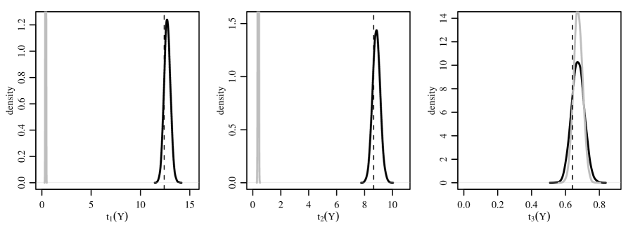
Figure 1: Posterior predictive distributions for summary statistics. The gray density represents is under the reduced model, the black under the full. The vertical dashed line is the observed value of the statistic.

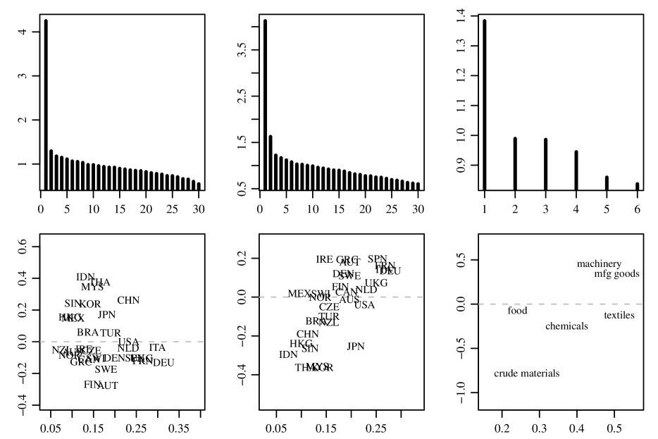
Figure 2: Estimates of correlation matrices corresponding to $\mathbf{\Sigma}_{1}$, $\mathbf{\Sigma}_{2}$ and $\mathbf{\Sigma}_{3}$. The first panel in each row plots the eigenvalues of each correlation matrix, the second plots the first two eigenvectors.

The fits of the two models can be compared using posterior predictive evaluations (Rubin, 1984): To evaluate the fit of a model, the observed value of a summary statistic $t(\mbox{\bf{Y}})$ can be compared to values $t(\tilde{\mbox{\bf{Y}}})$ for which $\tilde{\mbox{\bf{Y}}}$ is simulated from the posterior predictive distribution. A discrepancy between $t(\mbox{\bf{Y}})$ and the distribution of $t(\tilde{\mbox{\bf{Y}}})$ indicates that the model is not capturing the aspect of the data represented by $t(\cdot)$. For illustration, we use such checks here to evaluate evidence that $\mathbf{\Sigma}_{1}$ and $\mathbf{\Sigma}_{2}$ are not equal to the identity, or equivalently, that model 1 exhibits lack of fit as compared to model 2. To obtain a summary statistic evaluating evidence of a non-identity covariance matrix for $\mathbf{\Sigma}_{1}$, we first subtract the sample mean from the data array to obtain $\mbox{\bf{E}}=\mbox{\bf{Y}}-\bar{\mbox{\bf{Y}}}$, and then compute $\mbox{\boldmath{${\rm S}$}}_{1}=(\mbox{\bf{E}}_{(1)}\mbox{\bf{E}}_{(1)}^{T})$. The $m\times m$ matrix $\mbox{\boldmath{${\rm S}$}}_{1}$ is a sample measure of covariance among exporting countries. We then obtain a scaled version $\tilde{\mbox{\boldmath{${\rm S}$}}}_{1}=\mbox{\boldmath{${\rm S}$}}_{1}/{\rm tr}(\mbox{\boldmath{${\rm S}$}}_{1})$, and compare it to a scaled version of the identity matrix:

$$t_{1}(\mbox{\bf{Y}})=\log|\tilde{\mbox{\boldmath{${\rm S}$}}}_{1}|-\log|\mbox{\boldmath{${\rm I}$}}/m|=\log|\tilde{\mbox{\boldmath{${\rm S}$}}}_{1}|+m\log m.$$

Note that the minimum value of this statistic occurs when $\tilde{\mbox{\boldmath{${\rm S}$}}}_{1}=\mbox{\boldmath{${\rm I}$}}/m$, and so in some sense it provides a simple scalar measure of how the sample covariance among exporters differs from a scaled identity matrix. Similarly, we construct $t_{2}(\mbox{\bf{Y}})$ and $t_{3}(\mbox{\bf{Y}})$ measuring sample covariance along the second and third modes of the data array. We include $t_{3}$ to contrast with $t_{1}$ and $t_{2}$, as both the full and reduced models include covariance parameters for the third dimension of the array.

Figure 1 plots posterior predictive densities for $t_{1}(\tilde{\mbox{\bf{Y}}})$, $t_{2}(\tilde{\mbox{\bf{Y}}})$ and $t_{3}(\tilde{\mbox{\bf{Y}}})$ under both the full and reduced models, and compares these densities to the observed values of the statistics. The reduced model exhibits substantial lack of fit in terms of its inability to predict datasets that resemble the observed in terms of $t_{1}$ and $t_{2}$. In other words, a model that assumes i.i.d. structure along the first two modes of the array does not fit the data. In terms of covariance among commodities along the third mode, neither model exhibits substantial lack of fit as measured by $t_{3}$.

Figure 2 describes posterior mean estimates of the correlation matrices corresponding to $\mathbf{\Sigma}_{1}$, $\mathbf{\Sigma}_{2}$ and $\mathbf{\Sigma}_{3}$. The two panels in each column plot the eigenvalues and the first two eigenvectors each of the three correlation matrices. The eigenvalues for all three suggest the possibility of modeling the covariances matrices with factor analytic structure, i.e. letting $\mathbf{\Sigma}_{k}=\mbox{\boldmath{${\rm A}$}}\mbox{\boldmath{${\rm A}$}}^{T}+{\rm diag}(b_{1}^{2},\ldots,b_{m_{k}}^{2})$, where ${\rm A}$ is an $m_{k}\times r$ matrix with $r<m_{k}$. This possibility is described further in the Discussion. The second row of Figure 2 describes correlations among exporters, importers and commodities. The first two plots show that much of the correlation among exporters and among importers is related to geography, with countries having similar eigenvector values typically being near each other geographically. The third plot in the row indicates correlation among commodities of a similar type: Moving up and to the right from “crude materials,” the commodities are essentially in order of the extent to which they are finished goods.

5 Discussion

This article has proposed a class of array normal distributions with separable covariance structure for the modeling of array data, particularly multivariate relational arrays. It has been shown that the class of separable covariance models can be generated by a type of array-matrix multiplication known as the Tucker product. Maximum likelihood estimation and Bayesian inference in Gaussian versions of such models are feasible using relatively simple properties of array-matrix multiplication. These types of models can be useful for describing covariance within the index sets of an array dataset. In an example involving longitudinal trade data, we have shown that a full array normal model provides a better fit than a matrix normal model, which includes a covariance matrix for only two of the four modes of the data array.

One open area of research is finding conditions for the existence and uniqueness of the MLE for the array normal model. In fact, such conditions for even the simple matrix normal case are not fully established. Each step of the iterative MLE algorithm of Dutilleul (1999) is well defined as long as $n\geq\max\{m_{1}/m_{2},m_{2}/m_{1}\}+1$, suggesting that this condition might be sufficient to provide existence. Unfortunately, it is easy to find examples where this condition is met but the likelihood is unbounded, and no MLE exists. In contrast, Srivastava et al. (2008) show the MLE exists and is essentially unique if $n>\max\{m_{1},m_{2}\}$, a much stronger requirement. However, they do not show that this condition is necessary. Unpublished results of this author suggest that this latter condition can be relaxed, and that the existence of the MLE depends on the minimal possible rank of $\sum_{i=1}^{n}\mbox{\boldmath{${\rm Y}$}}_{i}\mbox{\boldmath{${\rm U}$}}_{k}\mbox{\boldmath{${\rm U}$}}_{k}^{T}\mbox{\boldmath{${\rm Y}$}}_{i}^{T}$ for $k\leq\min\{m_{1},m_{2}\}$, where $\mbox{\boldmath{${\rm U}$}}_{k}$ is an $m_{2}\times k$ matrix with orthonormal columns. However, such conditions are somewhat opaque, and it is not clear that they could easily be generalized to the array normal case.

A potentially useful model variation would be to consider imposing simplifying structure on the component matrices. For example, a normal factor analysis model for a random vector $\mbox{\boldmath{${\rm y}$}}\in\mathbb{R}^{p}$ posits that $\mbox{\boldmath{${\rm y}$}}=\mbox{\boldmath{${\rm\mu}$}}+\mbox{\boldmath{${\rm B}$}}\mbox{\boldmath{${\rm z}$}}+\mbox{\boldmath{${\rm D}$}}\mbox{\boldmath{${\rm\epsilon}$}}$ where $\mbox{\boldmath{${\rm z}$}}\in\mathbb{R}^{r},r<p$ and $\mbox{\boldmath{${\rm\epsilon}$}}\in\mathbb{R}^{p}$ are uncorrelated standard normal vectors and ${\rm D}$ is a diagonal matrix. The resulting covariance matrix is given by ${\rm Cov}[\mbox{\boldmath{${\rm y}$}}]=\mbox{\boldmath{${\rm B}$}}\mbox{\boldmath{${\rm B}$}}^{T}+\mbox{\boldmath{${\rm D}$}}^{2}$, in which the “interesting” part $\mbox{\boldmath{${\rm B}$}}\mbox{\boldmath{${\rm B}$}}^{T}$ is of rank $r$. The natural extension to random arrays is $\mbox{\bf{Y}}_{i}=\mbox{\bf{M}}+\mbox{\boldmath{${\rm Z}$}}\times\{\mbox{\boldmath{${\rm B}$}}_{1},\ldots,\mbox{\boldmath{${\rm B}$}}_{K}\}+\mbox{\boldmath{${\rm E}$}}\times\{\mbox{\boldmath{${\rm D}$}}_{1},\ldots,\mbox{\boldmath{${\rm D}$}}_{K}\}$ where $\mbox{\bf{Z}}\in\mathbb{R}^{r_{1}\times\cdots\times r_{K}}$ and $\mbox{\bf{E}}\in\mathbb{R}^{p_{1}\times\cdots\times p_{K}}$ are uncorrelated standard normal arrays. This induces the covariance matrix ${\rm Cov}[{\rm vec}(\mbox{\boldmath{${\rm Y}$}})]=(\mbox{\boldmath{${\rm B}$}}_{K}\mbox{\boldmath{${\rm B}$}}_{K}^{T})\otimes\cdots\otimes(\mbox{\boldmath{${\rm B}$}}_{1}\mbox{\boldmath{${\rm B}$}}_{1})^{T}+\mbox{\boldmath{${\rm D}$}}_{K}^{2}\otimes\cdots\otimes\mbox{\boldmath{${\rm D}$}}_{1}^{2}$. This is essentially the model-based analogue of the higher-order SVD of De Lathauwer et al. (2000), in the same way that the usual factor analysis model for vector-valued data is analogous to the matrix SVD. Alternatively, in some cases it may be desirable to fit a factor-analytic structure for the covariances of some modes of the array while estimating others as unstructured. This can be achieved with a model of the following form:

Y $$= \mbox{\bf{M}}+\mbox{\bf{Z}}\times\{\mathbf{\Sigma}_{1}^{1/2},\ldots,\mathbf{\Sigma}_{k}^{1/2},\mbox{\boldmath{${\rm B}$}}_{k+1},\ldots,\mbox{\boldmath{${\rm B}$}}_{K}\}+\mbox{\bf{E}}\times\{\mathbf{\Sigma}_{1}^{1/2},\ldots,\mathbf{\Sigma}_{k}^{1/2},\mbox{\boldmath{${\rm D}$}}_{k+1},\ldots,\mbox{\boldmath{${\rm D}$}}_{K}\}$$

where $\mbox{\bf{Z}}\in\mathbb{R}^{p_{1}\times\cdots p_{k}\times r_{k+1}\times\cdots r_{K}}$, and $\mbox{\bf{E}}\in\mathbb{R}^{p_{1}\times\cdots\times p_{K}}$. The resulting covariance for Y is given by

$${\rm Cov}[{\rm vec}(\mbox{\boldmath{${\rm Y}$}})]=(\mbox{\boldmath{${\rm B}$}}_{K}\mbox{\boldmath{${\rm B}$}}_{K}^{T}+\mbox{\boldmath{${\rm D}$}}_{K}^{2})\otimes\cdots\otimes(\mbox{\boldmath{${\rm B}$}}_{k+1}\mbox{\boldmath{${\rm B}$}}_{k+1}+\mbox{\boldmath{${\rm D}$}}_{k+1}^{2})^{T}\otimes\mathbf{\Sigma}_{k}\otimes\cdots\otimes\mathbf{\Sigma}_{1},$$

which is separable, and so is in the array normal class. Such a factor model may be useful if some modes of the array have very high dimensions, and rank-reduced estimates of the corresponding covariance matrices are desired.

An additional model extension would be to accommodate non-normal continuous or discrete array data, for example, dynamic binary networks. This can be done by embedding the array normal model within a generalized linear model, or within an ordered probit model for ordinal response data. For example, if Y is a three-way binary array, an array normal probit model would posit a latent array $\mbox{\bf{Z}}\sim{\rm anorm}(\mbox{\bf{M}},\mathbf{\Sigma}_{1}\circ\mathbf{\Sigma}_{2}\circ\mathbf{\Sigma}_{3})$ which determines Y via $y_{i,j,k}=\delta_{(0,\infty)}(z_{i,j,k})$.

Computer code and data for the example in Section 5 is available at my website: http://www.stat.washington.edu/~hoff.

Appendix

Proof of Proposition 3.1. Let $\mbox{\bf{Y}}=\mbox{\bf{Z}}\times{\mbox{\boldmath{${\rm A}$}}}$ where the elements of Z are uncorrelated, have expectation zero and variance one. Using the fact that $\mbox{\boldmath{${\rm Y}$}}_{(1)}=\mbox{\boldmath{${\rm A}$}}_{1}\mbox{\bf{Z}}_{(1)}\mbox{\boldmath{${\rm B}$}}^{T}$ where $\mbox{\boldmath{${\rm B}$}}=(\mbox{\bf{A}}_{K}\otimes\cdots\otimes\mbox{\bf{A}}_{2})$ (Kolda, 2006, Proposition 4.3), we have

$${\rm vec}(\mbox{\bf{Y}})={\rm vec}(\mbox{\bf{Y}}_{(1)}) = {\rm vec}(\mbox{\boldmath{${\rm A}$}}_{1}\mbox{\bf{Z}}_{(1)}\mbox{\bf{B}}^{T})$$

$$= (\mbox{\boldmath{${\rm B}$}}\otimes\mbox{\boldmath{${\rm A}$}}_{1}){\rm vec}(\mbox{\boldmath{${\rm Z}$}}_{(1)})=(\mbox{\boldmath{${\rm B}$}}\otimes\mbox{\boldmath{${\rm A}$}}_{1}){\rm vec}(\mbox{\boldmath{${\rm Z}$}}).$$

The covariance of ${\rm vec}(\mbox{\bf{Y}})$ is then

$${\rm E}[{\rm vec}(\mbox{\bf{Y}}){\rm vec}(\mbox{\bf{Y}})^{T}] = (\mbox{\boldmath{${\rm B}$}}\otimes\mbox{\boldmath{${\rm A}$}}_{1}){\rm E}[{\rm vec}(\mbox{\bf{Z}}){\rm vec}(\mbox{\bf{Z}})^{T}](\mbox{\boldmath{${\rm B}$}}\otimes\mbox{\boldmath{${\rm A}$}}_{1})^{T}$$

$$= (\mbox{\boldmath{${\rm A}$}}_{K}\otimes\cdots\otimes\mbox{\boldmath{${\rm A}$}}_{1})\mbox{\boldmath{${\rm I}$}}(\mbox{\boldmath{${\rm A}$}}_{K}\otimes\cdots\otimes\mbox{\boldmath{${\rm A}$}}_{1})^{T}$$

$$= (\mbox{\boldmath{${\rm A}$}}_{K}\mbox{\boldmath{${\rm A}$}}_{K}^{T})\otimes\cdots\otimes(\mbox{\boldmath{${\rm A}$}}_{1}\mbox{\boldmath{${\rm A}$}}_{1}^{T})$$

$$= \mathbf{\Sigma}_{K}\otimes\cdots\otimes\mathbf{\Sigma}_{1},$$

where $\mathbf{\Sigma}_{k}=\mbox{\boldmath{${\rm A}$}}_{k}\mbox{\boldmath{${\rm A}$}}_{k}^{T}$. This proves the second statement in the proposition. The first statement follows from how the “vec” operation is applied to arrays. For the third statement, consider the calculation of ${\rm E}[\mbox{\boldmath{${\rm Y}$}}_{(1)}\mbox{\boldmath{${\rm Y}$}}_{(1)}^{T}]$, again using the fact that $\mbox{\boldmath{${\rm Y}$}}_{(1)}=\mbox{\boldmath{${\rm A}$}}_{1}\mbox{\bf{Z}}_{(1)}\mbox{\boldmath{${\rm B}$}}^{T}$:

$${\rm E}[\mbox{\boldmath{${\rm Y}$}}_{(1)}\mbox{\boldmath{${\rm Y}$}}_{(1)}^{T}] = \mbox{\boldmath{${\rm A}$}}_{1}{\rm E}[\mbox{\boldmath{${\rm Z}$}}_{(1)}\mbox{\boldmath{${\rm B}$}}^{T}\mbox{\boldmath{${\rm B}$}}\mbox{\boldmath{${\rm Z}$}}_{(1)}^{T}]\mbox{\boldmath{${\rm A}$}}_{1}^{T}$$ (4)

$$= \mbox{\boldmath{${\rm A}$}}_{1}{\rm E}[\mbox{\boldmath{${\rm X}$}}\mbox{\boldmath{${\rm X}$}}^{T}]\mbox{\boldmath{${\rm A}$}}_{1}^{T},$$

where $\mbox{\boldmath{${\rm X}$}}=\mbox{\boldmath{${\rm Z}$}}_{(1)}\mbox{\boldmath{${\rm B}$}}^{T}$. Because the elements of ${\rm Z}$ are all independent, mean zero and variance one, the rows of ${\rm X}$ are independent with mean zero and variance $\mbox{\boldmath{${\rm B}$}}\mbox{\boldmath{${\rm B}$}}^{T}$. Thus ${\rm E}[\mbox{\boldmath{${\rm X}$}}\mbox{\boldmath{${\rm X}$}}^{T}]={\rm tr}(\mbox{\boldmath{${\rm B}$}}\mbox{\boldmath{${\rm B}$}}^{T})\mbox{\boldmath{${\rm I}$}}$. Combining this with (4) gives

$${\rm E}[\mbox{\boldmath{${\rm Y}$}}_{(1)}\mbox{\boldmath{${\rm Y}$}}_{(1)}^{T}] = \mbox{\boldmath{${\rm A}$}}_{1}\mbox{\boldmath{${\rm A}$}}_{1}^{T}{\rm tr}(\mbox{\boldmath{${\rm B}$}}\mbox{\boldmath{${\rm B}$}}^{T})$$

$$= \mbox{\boldmath{${\rm A}$}}_{1}\mbox{\boldmath{${\rm A}$}}_{1}^{T}{\rm tr}([\mbox{\boldmath{${\rm A}$}}_{K}\otimes\cdots\otimes\mbox{\boldmath{${\rm A}$}}_{2}][\mbox{\boldmath{${\rm A}$}}_{K}^{T}\otimes\cdots\otimes\mbox{\boldmath{${\rm A}$}}_{2}^{T}]$$

$$= \mathbf{\Sigma}_{1}{\rm tr}(\mathbf{\Sigma}_{K}\otimes\cdots\otimes\mathbf{\Sigma}_{1})$$

$$= \mathbf{\Sigma}_{1}\prod_{k=2}^{K}{\rm tr}(\mathbf{\Sigma}_{k}).$$

Calculation of ${\rm E}[\mbox{\boldmath{${\rm Y}$}}_{(k)}\mbox{\boldmath{${\rm Y}$}}_{(k)}^{T}]$ for other values of $k$ is similar. $\Box$

Proof of Proposition 3.2. We calculate ${\rm E}[{\rm vec}(\mbox{\bf{X}}){\rm vec}(\mbox{\bf{X}})^{T}]$ for the case that $\mbox{\bf{X}}=\mbox{\bf{Y}}\times_{1}\mbox{\boldmath{${\rm G}$}}$:

$${\rm vec}(\mbox{\bf{X}})={\rm vec}(\mbox{\bf{X}}_{(1)}) = {\rm vec}(\mbox{\boldmath{${\rm G}$}}\mbox{\bf{Y}}_{(1)})$$

$$= {\rm vec}(\mbox{\boldmath{${\rm G}$}}\mbox{\bf{Y}}_{(1)}\mbox{\boldmath{${\rm I}$}})$$

$$= (\mbox{\boldmath{${\rm I}$}}\otimes\mbox{\boldmath{${\rm G}$}}){\rm vec}(\mbox{\bf{Y}})\ ,\ \mbox{so}$$

$${\rm E}[{\rm vec}(\mbox{\bf{X}}){\rm vec}(\mbox{\bf{X}})^{T}] = (\mbox{\boldmath{${\rm I}$}}\otimes\mbox{\boldmath{${\rm G}$}}){\rm E}[{\rm vec}(\mbox{\bf{Y}}){\rm vec}(\mbox{\bf{Y}})^{T}](\mbox{\boldmath{${\rm I}$}}\otimes\mbox{\boldmath{${\rm G}$}})^{T}$$

$$= (\mbox{\boldmath{${\rm I}$}}\otimes\mbox{\boldmath{${\rm G}$}})(\mathbf{\Sigma}_{K}\otimes\cdots\otimes\mathbf{\Sigma}_{1})(\mbox{\boldmath{${\rm I}$}}\otimes\mbox{\boldmath{${\rm G}$}}^{T})$$

$$= [(\mathbf{\Sigma}_{K}\otimes\cdots\otimes\mathbf{\Sigma}_{2})\otimes(\mbox{\boldmath{${\rm G}$}}\mathbf{\Sigma}_{1})][\mbox{\boldmath{${\rm I}$}}\otimes\mbox{\boldmath{${\rm G}$}}^{T}]$$

$$= (\mathbf{\Sigma}_{K}\otimes\cdots\otimes\mathbf{\Sigma}_{2})\otimes(\mbox{\boldmath{${\rm G}$}}\mathbf{\Sigma}_{1}\mbox{\boldmath{${\rm G}$}}^{T}).$$

Calculation for the covariance of $\mbox{\bf{X}}=\mbox{\bf{Y}}\times_{k}\mbox{\boldmath{${\rm G}$}}$ for other values of $k$ proceeds analogously. $\Box$

Proof of Proposition 4.1 The density can be obtained as a re-expression of the density of $\mbox{\boldmath{${\rm e}$}}={\rm vec}(\mbox{\bf{E}})={\rm vec}(\mbox{\bf{Y}}-\mbox{\bf{M}})$, which has a multivariate normal distribution with mean zero and covariance $\mathbf{\Sigma}_{K}\otimes\cdots\otimes\mathbf{\Sigma}_{1}$. The re-expression is obtained using the following identities,

$$||(\mbox{\bf{Y}}-\mbox{\bf{M}})\times\mathbf{\Sigma}^{-1/2}||^{2} = \langle\mbox{\bf{E}},\mbox{\bf{E}}\times\mathbf{\Sigma}^{-1}\rangle$$

$$= {\rm vec}(\mbox{\bf{E}})^{T}{\rm vec}(\mbox{\bf{E}}\times\mathbf{\Sigma}^{-1})$$

$$= \mbox{\boldmath{${\rm e}$}}^{T}(\mathbf{\Sigma}_{K}\otimes\cdots\otimes\mathbf{\Sigma}_{1})^{-1}\mbox{\boldmath{${\rm e}$}}\ ,\ \mbox{and}$$

$$|\mathbf{\Sigma}_{K}\otimes\cdots\otimes\mathbf{\Sigma}_{1}| = \prod_{k=1}^{K}|\mathbf{\Sigma}_{k}|^{n_{k}},$$

where $n_{k}=\prod_{j:j\neq k}m_{j}$ is the number of columns of $\mbox{\boldmath{${\rm Y}$}}_{(k)}$, i.e. the “sample size” for $\mathbf{\Sigma}_{k}$. $\Box$

Proof of Proposition 4.3. We first obtain the full conditional distributions for the matrix normal case. Let $\mbox{\bf{Y}}\sim{\rm anorm}(\mbox{\bf{0}},\mathbf{\Sigma}\otimes\mathbf{\Omega})$ and $\mathbf{\Sigma}^{-1}=\mathbf{\Psi}$. Let $(\mbox{\boldmath{${\rm a}$}},\mbox{\boldmath{${\rm b}$}})$ form a partition of the row indices of Y, and assume the rows of Y are ordered according to this partition. The quadratic term in the exponent of the density can then be written as

$${\rm tr}(\mathbf{\Omega}^{-1}\mbox{\boldmath{${\rm Y}$}}^{T}\mathbf{\Psi}\mbox{\boldmath{${\rm Y}$}}) = {\rm tr}\left(\mathbf{\Omega}^{-1}(\mbox{\boldmath{${\rm Y}$}}_{a}^{T}\mbox{\boldmath{${\rm Y}$}}_{b}^{T})\left(\begin{array}[]{cc}\mathbf{\Psi}_{aa}&\mathbf{\Psi}_{ab}\\ \mathbf{\Psi}_{ba}&\mathbf{\Psi}_{bb}\end{array}\right)\left(\begin{array}[]{c}\mbox{\boldmath{${\rm Y}$}}_{a}\\ \mbox{\boldmath{${\rm Y}$}}_{b}\end{array}\right)\right)$$

$$= {\rm tr}(\mathbf{\Omega}^{-1}\mbox{\boldmath{${\rm Y}$}}_{a}^{T}\mathbf{\Psi}_{aa}\mbox{\boldmath{${\rm Y}$}}_{a})+2{\rm tr}(\mathbf{\Omega}^{-1}\mbox{\boldmath{${\rm Y}$}}_{b}^{T}\mathbf{\Psi}_{ba}\mbox{\boldmath{${\rm Y}$}}_{a})+{\rm tr}(\mathbf{\Omega}^{-1}\mbox{\boldmath{${\rm Y}$}}_{b}^{T}\mathbf{\Psi}_{bb}\mbox{\boldmath{${\rm Y}$}}_{b}).$$

As a function of $\mbox{\boldmath{${\rm Y}$}}_{b}$, this is equal to a constant plus the quadratic term of the matrix normal density with row and column covariance matrices of $\mathbf{\Psi}_{bb}^{-1}$ and $\mathbf{\Omega}$ , and a mean of $-\mathbf{\Omega}_{bb}^{-1}\mathbf{\Omega}_{ba}\mbox{\boldmath{${\rm Y}$}}_{a}$. Standard results on inverses of partitioned matrices give the row variance as $\mathbf{\Psi}_{bb}^{-1}=\mathbf{\Sigma}_{bb}-\mathbf{\Sigma}_{ba}(\mathbf{\Sigma}_{aa})^{-1}\mathbf{\Sigma}_{ab}=\mathbf{\Sigma}_{b|a}$ and the mean as $-\mathbf{\Omega}_{bb}^{-1}\mathbf{\Omega}_{ba}\mbox{\boldmath{${\rm Y}$}}_{a}=\mathbf{\Sigma}_{b|a}(\mathbf{\Sigma}_{aa})^{-1}\mbox{\boldmath{${\rm Y}$}}_{b}$. To obtain the result for the array case, note that if $\mbox{\bf{Y}}\sim{\rm anorm}(\mbox{\bf{0}},\mathbf{\Sigma}_{1}\circ\cdots\circ\mathbf{\Sigma}_{K})$ then the distribution of $\mbox{\bf{Y}}_{(1)}$ is matrix normal with row covariance $\mathbf{\Sigma}_{1}$ and column covariance $\mathbf{\Sigma}_{K}\otimes\cdots\otimes\mathbf{\Sigma}_{2}$. The conditional distribution can then be obtained by applying the result for the matrix normal case to $\mbox{\bf{Y}}_{(1)}$ with $\mathbf{\Sigma}=\mathbf{\Sigma}_{1}$ and $\mathbf{\Omega}=\mathbf{\Sigma}_{K}\otimes\cdots\otimes\mathbf{\Sigma}_{2}$. $\Box$

References

• Browne and Shapiro [1991] M. W. Browne and A. Shapiro. Invariance of covariance structures under groups of transformations. Metrika, 38(6):345–355, 1991. ISSN 0026-1335. doi: 10.1007/BF02613631. URL http://dx.doi.org/10.1007/BF02613631.
• Dawid [1981] A. P. Dawid. Some matrix-variate distribution theory: notational considerations and a Bayesian application. Biometrika, 68(1):265–274, 1981. ISSN 0006-3444. doi: 10.1093/biomet/68.1.265. URL http://dx.doi.org/10.1093/biomet/68.1.265.
• De Lathauwer et al. [2000] L. De Lathauwer, B. De Moor, and J. Vandewalle. A multilinear singular value decomposition. SIAM Journal on Matrix Analysis and Applications, 21(4):1253–1278, 2000.
• Dutilleul [1999] P Dutilleul. The mle algorithm for the matrix normal distribution. Journal of Statistical Computation and Simulation, 64(2):105–123, 1999.
• Galecki [1994] A.T. Galecki. General class of covariance structures for two or more repeated factors in longitudinal data analysis. Communications in Statistics-Theory and Methods, 23(11):3105–3119, 1994.
• Kass and Wasserman [1995] Robert E. Kass and Larry Wasserman. A reference Bayesian test for nested hypotheses and its relationship to the Schwarz criterion. J. Amer. Statist. Assoc., 90(431):928–934, 1995. ISSN 0162-1459.
• Kolda [2006] Tamara G. Kolda. Multilinear operators for higher-order decompositions. Technical Report SAND2006-2081, Sandia National Laboratories, Albuquerque, NM and Livermore, CA, April 2006.
• Lu and Zimmerman [2005] Nelson Lu and Dale L. Zimmerman. The likelihood ratio test for a separable covariance matrix. Statist. Probab. Lett., 73(4):449–457, 2005. ISSN 0167-7152. doi: 10.1016/j.spl.2005.04.020. URL http://dx.doi.org/10.1016/j.spl.2005.04.020.
• Mitchell et al. [2006] Matthew W. Mitchell, Marc G. Genton, and Marcia L. Gumpertz. A likelihood ratio test for separability of covariances. J. Multivariate Anal., 97(5):1025–1043, 2006. ISSN 0047-259X. doi: 10.1016/j.jmva.2005.07.005. URL http://dx.doi.org/10.1016/j.jmva.2005.07.005.
• Roy and Khattree [2005] Anuradha Roy and Ravindra Khattree. On implementation of a test for Kronecker product covariance structure for multivariate repeated measures data. Stat. Methodol., 2(4):297–306, 2005. ISSN 1572-3127. doi: 10.1016/j.stamet.2005.07.003. URL http://dx.doi.org/10.1016/j.stamet.2005.07.003.
• Rubin [1984] Donald B. Rubin. Bayesianly justifiable and relevant frequency calculations for the applied statistician. Ann. Statist., 12(4):1151–1172, 1984. ISSN 0090-5364. doi: 10.1214/aos/1176346785. URL http://dx.doi.org/10.1214/aos/1176346785.
• Srivastava et al. [2008] M.S. Srivastava, T. von Rosen, and D. Von Rosen. Models with a kronecker product covariance structure: estimation and testing. Mathematical Methods of Statistics, 17(4):357–370, 2008.
• Tseng [2001] P. Tseng. Convergence of a block coordinate descent method for nondifferentiable minimization. J. Optim. Theory Appl., 109(3):475–494, 2001. ISSN 0022-3239. doi: 10.1023/A:1017501703105. URL http://dx.doi.org/10.1023/A:1017501703105.
• Tucker [1964] L. R. Tucker. The extension of factor analysis to three-dimensional matrices. Contributions to mathematical psychology, pages 109–127, 1964.
• Tucker [1966] L.R. Tucker. Some mathematical notes on three-mode factor analysis. Psychometrika, 31(3):279–311, 1966.