Fractional pure birth processes

Abstract

We consider a fractional version of the classical nonlinear birth process of which the Yule–Furry model is a particular case. Fractionality is obtained by replacing the first order time derivative in the difference-differential equations which govern the probability law of the process with the Dzherbashyan–Caputo fractional derivative. We derive the probability distribution of the number $\mathcal{N}_{\nu}(t)$ of individuals at an arbitrary time $t$. We also present an interesting representation for the number of individuals at time $t$, in the form of the subordination relation $\mathcal{N}_{\nu}(t)=\mathcal{N}(T_{2\nu}(t))$, where $\mathcal{N}(t)$ is the classical generalized birth process and $T_{2\nu}(t)$ is a random time whose distribution is related to the fractional diffusion equation. The fractional linear birth process is examined in detail in Section 3 and various forms of its distribution are given and discussed.

and

1 Introduction

We consider a birth process and denote by $\mathcal{N}(t)$, $t>0$, the number of components in a stochastically developing population at time $t$. Possible examples are the number of particles produced in a radioactive disintegration and the number of particles in a cosmic ray shower where death is not permitted. The probabilities $p_{k}(t)=\operatorname{Pr}\{\mathcal{N}(t)=k\}$ satisfy the difference-differential equations

$$\frac{\mathrm{d}p_{k}}{\mathrm{d}t}=-\lambda_{k}p_{k}+\lambda_{k-1}p_{k-1},\qquad k\geq 1,$$ (1)

where, at time $t=0$,

$$p_{k}(0)=\cases{1,&\quad$k=1,$\cr 0,&\quad$k\geq 2.$}$$ (2)

This means that we initially have one progenitor igniting the branching process. For information on this process, consult Gikhman and Skorokhod [5], page 322.

Here, we will examine a fractional version of the birth process where the probabilities are governed by

$$\frac{\mathrm{d}^{\nu}p_{k}}{\mathrm{d}t^{\nu}}=-\lambda_{k}p_{k}+\lambda_{k-1}p_{k-1},\qquad k\geq 1,$$ (3)

and where the fractional derivative is understood in the Dzherbashyan–Caputo sense, that is, as

$$\frac{\mathrm{d}^{\nu}p_{k}}{\mathrm{d}t^{\nu}}=\frac{1}{\Gamma(1-\nu)}\int_{0}^{t}\frac{({\mathrm{d}}/{\mathrm{d}s})p_{k}(s)}{(t-s)^{\nu}}\,\mathrm{d}s\qquad\mbox{for $0<\nu<1$}$$ (4)

(see Podlubny [12]). The use of a Dzherbashyan–Caputo derivative is preferred because in this case, initial conditions can be expressed in terms of integer-order derivatives.

Extensions of continuous-time point processes like the homogeneous Poisson process to the fractional case have been considered in Jumarie [7], Cahoy [3], Laskin [9], Wang and Wen [17], Wang, Wen and Zhang [18], Wang, Zhang and Fan [19], Uchaikin and Sibatov [15], Repin and Saichev [13] and Beghin and Orsingher [2]. A recently published paper (Uchaikin, Cahoy and Sibatov [16]) considers a fractional version of the Yule–Furry process where the mean value $\mathbb{E}N_{\nu}(t)$ is analyzed.

By recursively solving equation (3) (we write $p_{k}(t)$, $t>0$, in equations (3) and $p_{k}^{\nu}(t)$ for the solutions), we obtain that

$$p_{k}^{\nu}(t) = \operatorname{Pr}\{\mathcal{N}_{\nu}(t)=k\}$$

$$= \cases{\displaystyle\prod_{j=1}^{k-1}\lambda_{j}\sum_{m=1}^{k}\biggl{\{}\frac{1}{\prod_{l=1,l\neq m}^{k}(\lambda_{l}-\lambda_{m})}E_{\nu,1}(-\lambda_{m}t^{\nu})\biggr{\}},&\quad$k>1,$\vspace*{2pt}\cr E_{\nu,1}(-\lambda_{1}t^{\nu}),&\quad$k=1.$}$$

Result (1) generalizes the classical distribution of the birth process (see Gikhman and Skorokhod [5], page 322, or Bartlett [1], page 59), where, instead of the exponentials, we have the Mittag–Leffler functions, defined as

$$E_{\nu,1}(x)=\sum_{h=0}^{\infty}\frac{x^{h}}{\Gamma(\nu h+1)},\qquad x\in\mathbb{R},\nu>0.$$ (6)

The fractional pure birth process has some specific features entailed by the fractional derivative appearing in (4), which is a non-local operator. The process governed by fractional equations (and therefore the related probabilities $p_{k}^{\nu}(t)=\operatorname{Pr}\{N_{\nu}(t)=k\},k\geq 1$) displays a slowly decreasing memory which seems a characteristic feature of all real systems (for example, the hereditariety and the related aspects observed in phenomena such as metal fatigue, magnetic hysteresis and others). Fractional equations of various types have proven to be useful in representing different phenomena in optics (light propagation through random media), transport of charge carriers and also in economics (a survey of applications can be found in Podlubny [12]). Below, we show that for the linear birth process $N_{\nu}(t),t>0,$ the mean values $\mathbb{E}N_{\nu}(t)$, $\operatorname{\mathbb{V}ar}N_{\nu}(t)$ are increasing functions as the order of fractionality $\nu$ decreases. This shows that the fractional birth process is capable of representing explosively developing epidemics, accelerated cosmic showers and, in general, very rapidly expanding populations. This is a feature which the fractional pure birth process shares with its Poisson fractional counterpart whose practical applications have been studied in recent works (see, for example, Laskin [9] and Cahoy [3]).

We are able to show that the fractional birth process $\mathcal{N}_{\nu}(t)$ can be represented as

$$\mathcal{N}_{\nu}(t)=\mathcal{N}(T_{2\nu}(t)),\qquad t>0,0<\nu\leq 1,$$ (7)

where $T_{2\nu}(t)$, $t>0$, is the random time process whose distribution at time $t$ is obtained from the fundamental solution to the fractional diffusion equation (the fractional derivative is defined in (4))

$${\displaystyle\frac{\partial^{2\nu}u}{\partial t^{2\nu}}}={\displaystyle\frac{\partial^{2}u}{\partial s^{2}}},\qquad 0<\nu\leq 1,$$ (8)

subject to the initial conditions $u(s,0)=\delta(s)$ for $0<\nu\leq 1$ and also $u_{t}(s,0)=0$ for $1/2<\nu\leq 1$, as

$$\operatorname{Pr}\{T_{2\nu}(t)\in\mathrm{d}s\}=\cases{2u_{2\nu}(s,t)\,\mathrm{d}s&\quad$\mbox{for }s>0,$\cr 0&\quad$\mbox{for }s<0.$}$$ (9)

This means that the fractional birth process is a classical birth process with a random time $T_{2\nu}(t)$ which is the sole component of (7) affected by the fractional derivative. In equation (8) and throughout the whole paper, the fractional derivative must be understood in the Dzherbashyan–Caputo sense (3). The representation (7) leads to

$$\operatorname{Pr}\{\mathcal{N}_{\nu}(t)=k\}=\int_{0}^{\infty}\operatorname{Pr}\{\mathcal{N}(s)=k\}\operatorname{Pr}\{T_{2\nu}(t)\in\mathrm{d}s\},$$ (10)

where

$$\operatorname{Pr}\{\mathcal{N}(s)=k\}=\cases{\displaystyle\prod_{j=1}^{k-1}\lambda_{j}\sum_{m=1}^{k}\frac{\mathrm{e}^{-\lambda_{m}s}}{\prod_{l=1,l\neq m}^{k}(\lambda_{l}-\lambda_{m})},&\quad$k>1$, $s>0,$\vspace*{2pt}\cr\mathrm{e}^{-\lambda_{1}s},&\quad$k=1$, $s>0.$}$$ (11)

Formula (10) immediately shows that $\sum_{k}\operatorname{Pr}\{\mathcal{N}_{\nu}(t)=k\}=1$ if and only if$\sum_{k}\operatorname{Pr}\{\mathcal{N}(t)=k\}=1$. It is well known that the process $\mathcal{N}(t)$, $t>0$, is such that $\operatorname{Pr}(\mathcal{N}(t)<\infty)=1$ for all $t>0$ (non-exploding) if $\sum_{k}\lambda_{k}^{-1}=\infty$ (see Feller [4], page 452).

A special case of the above fractional birth process is the fractional linear birth process where $\lambda_{k}=\lambda k$. In this case, the distribution (1) reduces to the simple form

$$p_{k}^{\nu}(t)=\sum_{j=1}^{k}\pmatrix{{k-1}\cr{j-1}}(-1)^{j-1}E_{\nu,1}(-\lambda jt^{\nu}),\qquad k\geq 1,t>0.$$ (12)

For $\nu=1$, we retrieve from (12) the classical geometric structure of the linear birth process with a single progenitor, that is,

$$p_{k}^{1}(t)=(1-\mathrm{e}^{-\lambda t})^{k-1}\mathrm{e}^{-\lambda t},\qquad k\geq 1,t>0.$$ (13)

An interesting qualitative feature of the fractional linear birth process can be extracted from (12); it permits us to highlight the dependence of the branching speed on the order of fractionality $\nu$. We show in Section 3 that

$$\operatorname{Pr}\{N_{\nu}(\mathrm{d}t)=n_{0}+1|N_{\nu}(0)=n_{0}\}\sim\frac{\lambda n_{0}(\mathrm{d}t)^{\nu}}{\Gamma(\nu+1)}$$ (14)

and this proves that a decrease in the order of fractionality $\nu$ speeds up the reproduction of individuals. We are not able to generalize (14) to the case

$$\operatorname{Pr}\{N_{\nu}(t+\mathrm{d}t)=n_{0}+1|N_{\nu}(t)=n_{0}\}$$ (15)

because the process we are investigating is not time-homogeneous. For the fractional linear birth process, the representation (7) reduces to the form

$$N_{\nu}(t)=N(T_{2\nu}(t)),\qquad t>0,0<\nu\leq 1,$$ (16)

and has an interesting special structure when $\nu=1/2^{n}$. For example, for $n=2$, the random time appearing in (16) becomes a folded iterated Brownian motion. This means that

$$N_{{1}/{4}}(t)=N(|\mathcal{B}_{1}(|\mathcal{B}_{2}(t)|)|).$$ (17)

Clearly, $|\mathcal{B}_{2}(t)|$ is a reflecting Brownian motion starting from zero and $|\mathcal{B}_{1}(|\mathcal{B}_{2}(t)|)|$ is a reflecting iterated Brownian motion. This permits us to write the distribution of (17) in the following form:

$$\operatorname{Pr}\{N_{{1}/{4}}(t)=k|N_{{1}/{4}}(0)=1\}$$

(18)

$$\quad=\int_{0}^{\infty}(1-\mathrm{e}^{-\lambda s})^{k-1}\mathrm{e}^{-\lambda s}\biggl{\{}2^{2}\int_{0}^{\infty}\frac{\mathrm{e}^{-{s^{2}}/{(4\omega)}}}{\sqrt{2\uppi 2\omega}}\frac{\mathrm{e}^{-{\omega^{2}}/{(4t)}}}{\sqrt{2\uppi 2t}}\,\mathrm{d}\omega\biggr{\}}\,\mathrm{d}s.$$

The case $\nu=1/2^{n}$ involves the $(n-1)$-times iterated Brownian motion

$$\mathcal{I}_{n-1}(t)=\mathcal{B}_{1}(|\mathcal{B}_{2}(\cdots|\mathcal{B}_{n}(t)|\cdots)|)$$ (19)

with distribution

$$\operatorname{Pr}\{|\mathcal{B}_{1}(|\mathcal{B}_{2}(\cdots|\mathcal{B}_{n}(t)|\cdots))|\in\mathrm{d}s\}$$

(20)

$$\quad=\mathrm{d}s2^{n}\int_{0}^{\infty}\frac{\mathrm{e}^{-{s^{2}}/{(4\omega_{1})}}}{\sqrt{4\uppi\omega_{1}}}\,\mathrm{d}\omega_{1}\int_{0}^{\infty}\frac{\mathrm{e}^{-{\omega_{1}^{2}}/{(4\omega_{2})}}}{\sqrt{4\uppi\omega_{2}}}\,\mathrm{d}\omega_{2}\cdots\int_{0}^{\infty}\frac{\mathrm{e}^{-{\omega_{n-1}^{2}}/{(4t)}}}{\sqrt{4\uppi t}}\,\mathrm{d}\omega_{n-1}.$$

For details on this point, see Orsingher and Beghin [11].

2 The distribution function for the generalized fractional birth process

We now present the explicit distribution

$$\operatorname{Pr}\{\mathcal{N}_{\nu}(t)=k|\mathcal{N}_{\nu}(0)=1\}=p_{k}^{\nu}(t),\qquad t>0,k\geq 1,0<\nu\leq 1,$$ (21)

of the number of individuals in the population expanding according to (3). Our technique is based on successive applications of the Laplace transform. Our first result is the following theorem.

Theorem 1

The solution to the fractional equations

$$\cases{\displaystyle\frac{\mathrm{d}^{\nu}p_{k}}{\mathrm{d}t^{\nu}}=-\lambda_{k}p_{k}+\lambda_{k-1}p_{k-1},&\quad$k\geq 1,0<\nu\leq 1,$\cr p_{k}(0)=\cases{1,&\quad$k=1,$\cr 0,&\quad$k\geq 2,$}&}$$ (22)

is given by

$$p_{k}^{\nu}(t) = \operatorname{Pr}\{\mathcal{N}_{\nu}(t)=k|\mathcal{N}_{\nu}(0)=1\}$$

$$= \cases{\displaystyle\prod_{j=1}^{k-1}\lambda_{j}\sum_{m=1}^{k}\biggl{\{}\frac{1}{\prod_{l=1,l\neq m}^{k}(\lambda_{l}-\lambda_{m})}E_{\nu,1}(-\lambda_{m}t^{\nu})\biggr{\}},&\quad$k>1,$\cr E_{\nu,1}(-\lambda_{1}t^{\nu}),&\quad$k=1$.}$$

Proof.

We prove the result (1) by a recursive procedure.

For $k=1$, the equation

$$\frac{\mathrm{d}^{\nu}p_{1}}{\mathrm{d}t^{\nu}}=-\lambda_{1}p_{1},\qquad p_{1}(0)=1,$$ (24)

is immediately solved by

$$p_{1}^{\nu}(t)=E_{\nu,1}(-\lambda_{1}t^{\nu}).$$ (25)

For $k=2$, equation (3) becomes

$$\cases{{\displaystyle\frac{\mathrm{d}^{\nu}p_{2}}{\mathrm{d}t^{\nu}}}=-\lambda_{2}p_{2}+\lambda_{1}E_{\nu,1}(-\lambda_{1}t^{\nu}),\vspace*{2pt}\cr p_{2}(0)=0.}$$ (26)

In view of the fact that

$$\int_{0}^{\infty}\mathrm{e}^{-\mu t}E_{\nu,1}(-\lambda_{1}t^{\nu})\,\mathrm{d}t=\frac{\mu^{\nu-1}}{\mu^{\nu}+\lambda_{1}},$$ (27)

the Laplace transform of (26) yields

$$L_{2}(\mu)=\frac{\lambda_{1}\mu^{\nu-1}}{\lambda_{2}-\lambda_{1}}\biggl{[}\frac{1}{\mu^{\nu}+\lambda_{1}}-\frac{1}{\mu^{\nu}+\lambda_{2}}\biggr{]}.$$ (28)

In the light of (27), from (28), we can determine the probability $p_{2}^{\nu}(t)$:

$$p_{2}^{\nu}(t)=[E_{\nu,1}(-\lambda_{1}t^{\nu})-E_{\nu,1}(-\lambda_{2}t^{\nu})]\frac{\lambda_{1}}{\lambda_{2}-\lambda_{1}}.$$ (29)

Now, the Laplace transform of

$$\frac{\mathrm{d}^{\nu}p_{3}}{\mathrm{d}t^{\nu}}=-\lambda_{3}p_{3}+\frac{\lambda_{2}\lambda_{1}}{\lambda_{2}-\lambda_{1}}[E_{\nu,1}(-\lambda_{1}t^{\nu})-E_{\nu,1}(-\lambda_{2}t^{\nu})]$$ (30)

yields, after some computation,

$$L_{3}(\mu)=\lambda_{2}\lambda_{1}\mu^{\nu-1}\biggl{[}\frac{1}{(\lambda_{2}-\lambda_{1})(\lambda_{3}-\lambda_{1})}\frac{1}{\mu^{\nu}+\lambda_{1}}$$

$$\phantom{L_{3}(\mu)=\lambda_{2}\lambda_{1}\mu^{\nu-1}\biggl{[}}{}+\frac{1}{(\lambda_{1}-\lambda_{2})(\lambda_{3}-\lambda_{2})}\frac{1}{\mu^{\nu}+\lambda_{2}}$$ (31)

$$\phantom{L_{3}(\mu)=\lambda_{2}\lambda_{1}\mu^{\nu-1}\biggl{[}}{}+\frac{1}{(\lambda_{1}-\lambda_{3})(\lambda_{2}-\lambda_{3})}\frac{1}{\mu^{\nu}+\lambda_{3}}\biggr{]}.\vspace*{2pt}$$

From this result, it is clear that

$$p_{3}^{\nu}(t)=\lambda_{2}\lambda_{1}\biggl{[}\frac{1}{(\lambda_{2}-\lambda_{1})(\lambda_{3}-\lambda_{1})}E_{\nu,1}(-\lambda_{1}t^{\nu})$$

$$\phantom{p_{3}^{\nu}(t)=\lambda_{2}\lambda_{1}\biggl{[}}{}+\frac{1}{(\lambda_{1}-\lambda_{2})(\lambda_{3}-\lambda_{2})}E_{\nu,1}(-\lambda_{2}t^{\nu})$$ (32)

$$\phantom{p_{3}^{\nu}(t)=\lambda_{2}\lambda_{1}\biggl{[}}{}+\frac{1}{(\lambda_{1}-\lambda_{3})(\lambda_{2}-\lambda_{3})}E_{\nu,1}(-\lambda_{3}t^{\nu})\biggr{]}.\vspace*{2pt}$$

The procedure for $k>3$ becomes more complicated. However, the special case $k=4$ is instructive and so we treat it first.

The Laplace transform of the equation

$$\frac{\mathrm{d}^{\nu}p_{4}}{\mathrm{d}t^{\nu}}=-\lambda_{4}p_{4}+\lambda_{1}\lambda_{2}\lambda_{3}\biggl{[}\frac{1}{(\lambda_{2}-\lambda_{1})(\lambda_{3}-\lambda_{1})}E_{\nu,1}(-\lambda_{1}t^{\nu})$$

$$\phantom{\frac{\mathrm{d}^{\nu}p_{4}}{\mathrm{d}t^{\nu}}=-\lambda_{4}p_{4}+\lambda_{1}\lambda_{2}\lambda_{3}\biggl{[}}{}+\frac{1}{(\lambda_{1}-\lambda_{2})(\lambda_{3}-\lambda_{2})}E_{\nu,1}(-\lambda_{2}t^{\nu})$$ (33)

$$\phantom{\frac{\mathrm{d}^{\nu}p_{4}}{\mathrm{d}t^{\nu}}=-\lambda_{4}p_{4}+\lambda_{1}\lambda_{2}\lambda_{3}\biggl{[}}{}+\frac{1}{(\lambda_{1}-\lambda_{3})(\lambda_{2}-\lambda_{3})}E_{\nu,1}(-\lambda_{2}t^{\nu})\biggr{]},\vspace*{2pt}$$

subject to the initial condition $p_{4}(0)=0$, becomes

$$L_{4}(\mu)=\lambda_{1}\lambda_{2}\lambda_{3}\mu^{\nu-1}\biggl{[}\frac{1}{(\lambda_{2}-\lambda_{1})(\lambda_{3}-\lambda_{1})(\lambda_{4}-\lambda_{1})}\biggl{\{}\frac{1}{\mu^{\nu}+\lambda_{1}}-\frac{1}{\mu^{\nu}+\lambda_{4}}\biggr{\}}$$

$$\phantom{L_{4}(\mu)=\lambda_{1}\lambda_{2}\lambda_{3}\mu^{\nu-1}\biggl{[}}{}+\frac{1}{(\lambda_{1}-\lambda_{2})(\lambda_{3}-\lambda_{2})(\lambda_{4}-\lambda_{2})}\biggl{\{}\frac{1}{\mu^{\nu}+\lambda_{2}}-\frac{1}{\mu^{\nu}+\lambda_{4}}\biggr{\}}$$ (34)

$$\phantom{L_{4}(\mu)=\lambda_{1}\lambda_{2}\lambda_{3}\mu^{\nu-1}\biggl{[}}{}+\frac{1}{(\lambda_{1}-\lambda_{3})(\lambda_{2}-\lambda_{3})(\lambda_{4}-\lambda_{3})}\biggl{\{}\frac{1}{\mu^{\nu}+\lambda_{3}}-\frac{1}{\mu^{\nu}+\lambda_{4}}\biggr{\}}\biggr{]}.\qquad$$

The critical point of the proof is to show that

$$-\bigl{(}(\lambda_{3}-\lambda_{2})(\lambda_{4}-\lambda_{2})(\lambda_{4}-\lambda_{3})-(\lambda_{3}-\lambda_{1})(\lambda_{4}-\lambda_{1})(\lambda_{4}-\lambda_{3})$$

$$\qquad{}+(\lambda_{2}-\lambda_{1})(\lambda_{4}-\lambda_{1})(\lambda_{4}-\lambda_{2})\bigr{)}$$

(35)

$$\qquad{}\times\frac{1}{(\lambda_{2}-\lambda_{1})(\lambda_{3}-\lambda_{1})(\lambda_{4}-\lambda_{1})(\lambda_{3}-\lambda_{2})(\lambda_{4}-\lambda_{2})(\lambda_{4}-\lambda_{3})}$$

$$\quad=\frac{1}{(\lambda_{1}-\lambda_{4})(\lambda_{2}-\lambda_{4})(\lambda_{3}-\lambda_{4})}.$$

We note that

$$0 = \det\pmatrix{1&1&1&1\cr 1&1&1&1\cr\lambda_{1}&\lambda_{2}&\lambda_{3}&\lambda_{4}\vspace*{2pt}\cr\lambda_{1}^{2}&\lambda_{2}^{2}&\lambda_{3}^{2}&\lambda_{4}^{2}}$$

$$= \det\pmatrix{1&1&1\cr\lambda_{2}&\lambda_{3}&\lambda_{4}\vspace*{2pt}\cr\lambda_{2}^{2}&\lambda_{3}^{2}&\lambda_{4}^{2}}$$

$${}-\det\pmatrix{1&1&1\cr\lambda_{1}&\lambda_{3}&\lambda_{4}\vspace*{2pt}\cr\lambda_{1}^{2}&\lambda_{3}^{2}&\lambda_{4}^{2}}+\det\pmatrix{1&1&1\cr\lambda_{1}&\lambda_{2}&\lambda_{4}\vspace*{2pt}\cr\lambda_{1}^{2}&\lambda_{2}^{2}&\lambda_{4}^{2}}-\det\pmatrix{1&1&1\cr\lambda_{1}&\lambda_{2}&\lambda_{3}\vspace*{2pt}\cr\lambda_{1}^{2}&\lambda_{2}^{2}&\lambda_{3}^{2}}$$

$$= (\lambda_{3}-\lambda_{2})(\lambda_{4}-\lambda_{2})(\lambda_{4}-\lambda_{3})-(\lambda_{3}-\lambda_{1})(\lambda_{4}-\lambda_{1})(\lambda_{4}-\lambda_{3})$$

$${}+(\lambda_{2}-\lambda_{1})(\lambda_{4}-\lambda_{1})(\lambda_{4}-\lambda_{2})-(\lambda_{2}-\lambda_{1})(\lambda_{3}-\lambda_{1})(\lambda_{3}-\lambda_{2}),$$

where, in the last step, the Vandermonde formula is applied.

By inserting (2) into (2), we now have that

$$L_{4}(\mu)=\lambda_{1}\lambda_{2}\lambda_{3}\mu^{\nu-1}\biggl{[}\frac{1}{(\lambda_{2}-\lambda_{1})(\lambda_{3}-\lambda_{1})(\lambda_{4}-\lambda_{1})}\frac{1}{\mu^{\nu}+\lambda_{1}}$$

$$\phantom{L_{4}(\mu)=\lambda_{1}\lambda_{2}\lambda_{3}\mu^{\nu-1}\biggl{[}}{}+\frac{1}{(\lambda_{1}-\lambda_{2})(\lambda_{3}-\lambda_{2})(\lambda_{4}-\lambda_{2})}\frac{1}{\mu^{\nu}+\lambda_{2}}$$

(37)

$$\phantom{L_{4}(\mu)=\lambda_{1}\lambda_{2}\lambda_{3}\mu^{\nu-1}\biggl{[}}{}+\frac{1}{(\lambda_{1}-\lambda_{3})(\lambda_{2}-\lambda_{3})(\lambda_{4}-\lambda_{3})}\frac{1}{\mu^{\nu}+\lambda_{3}}$$

$$\phantom{L_{4}(\mu)=\lambda_{1}\lambda_{2}\lambda_{3}\mu^{\nu-1}\biggl{[}}{}+\frac{1}{(\lambda_{1}-\lambda_{4})(\lambda_{2}-\lambda_{4})(\lambda_{3}-\lambda_{4})}\frac{1}{\mu^{\nu}+\lambda_{4}}\biggr{]}$$

so that by inverting (2), we obtain the following result:

$$p_{4}^{\nu}(t)=\prod_{j=1}^{3}\lambda_{j}\Biggl{\{}\sum_{m=1}^{4}\frac{1}{\prod_{l=1,l\neq m}^{4}(\lambda_{l}-\lambda_{m})}E_{\nu,1}(-\lambda_{m}t^{\nu})\Biggr{\}}.$$ (38)

We now tackle the problem of showing that (1) solves the Cauchy problem (22) for all $k>1$, by induction. This means that we must solve

$$\cases{{\displaystyle\frac{\mathrm{d}^{\nu}p_{k}}{\mathrm{d}t^{\nu}}}=-\lambda_{k}p_{k}+\displaystyle\prod_{j=1}^{k-1}\lambda_{j}\Biggl{\{}\sum_{m=1}^{k-1}\frac{1}{\prod_{l=1,l\neq m}^{k-1}(\lambda_{l}-\lambda_{m})}E_{\nu,1}(-\lambda_{m}t^{\nu})\Biggr{\}},\cr p_{k}(0)=0,}\qquad k>4.$$ (39)

The Laplace transform of (39) reads

$$L_{k}(\mu)=\prod_{j=1}^{k-1}\lambda_{j}\Biggl{[}\sum_{m=1}^{k-1}\frac{\mu^{\nu-1}}{\prod_{l=1,l\neq m}^{k}(\lambda_{l}-\lambda_{m})}\frac{1}{\mu^{\nu}+\lambda_{m}}$$

(40)

$$\phantom{L_{k}(\mu)=\prod_{j=1}^{k-1}\lambda_{j}\Biggl{[}}{}-\frac{\mu^{\nu-1}}{\mu^{\nu}+\lambda_{k}}\sum_{m=1}^{k-1}\frac{1}{\prod_{l=1,l\neq m}^{k}(\lambda_{l}-\lambda_{m})}\Biggr{]}.$$

We must now prove that

$$-\sum_{m=1}^{k-1}\frac{1}{\prod_{l=1,l\neq m}^{k}(\lambda_{l}-\lambda_{m})}=\frac{1}{\prod_{l=1,l\neq k}^{k}(\lambda_{l}-\lambda_{k})}$$ (41)

and this relation is also important for the proof of (11).

In order to prove (41), we rewrite the left-hand side as

$$-\sum_{m=1}^{k-1}\frac{\prod_{h=1}^{k-1}\prod_{l>h}^{k}(\lambda_{l}-\lambda_{h})}{\prod_{l=1,l\neq m}^{k}(\lambda_{l}-\lambda_{m})}\cdot\frac{1}{\prod_{h=1}^{k-1}\prod_{l>h}^{k}(\lambda_{l}-\lambda_{h})}$$ (42)

and concentrate our attention on the numerator of (42). By analogy with the calculations in (2), we have that

$$0 = \det\pmatrix{1&1&\cdots&1&\cdots&1\cr 1&1&\cdots&1&\cdots&1\cr\lambda_{1}&\lambda_{2}&\cdots&\lambda_{m}&\cdots&\lambda_{k}\cr\cdots&\cdots&\cdots&\cdots&\cdots&\cdots\cr\lambda_{1}^{k-2}&\lambda_{2}^{k-2}&\cdots&\lambda_{m}^{k-2}&\cdots&\lambda_{k}^{k-2}}$$

$$= \sum_{m=1}^{k}(-1)^{m-1}\det\pmatrix{1&\cdots&1&1&\cdots&1\cr\lambda_{1}&\cdots&\lambda_{m-1}&\lambda_{m+1}&\cdots&\lambda_{k}\vspace*{2pt}\cr\lambda_{1}^{k-2}&\cdots&\lambda_{m-1}^{k-2}&\lambda_{m+1}^{k-2}&\cdots&\lambda_{k}^{k-2}}$$

$$= \sum_{m=1}^{k}\frac{\prod_{h=1}^{k-1}\prod_{l>h}^{k}(\lambda_{l}-\lambda_{h})}{\prod_{l=1,l\neq m}^{k}(\lambda_{l}-\lambda_{m})}=\sum_{m=1}^{k-1}\frac{\prod_{h=1}^{k-1}\prod_{l>h}^{k}(\lambda_{l}-\lambda_{h})}{\prod_{l=1,l\neq m}^{k}(\lambda_{l}-\lambda_{m})}+\frac{\prod_{h=1}^{k-1}\prod_{l>h}^{k}(\lambda_{l}-\lambda_{h})}{\prod_{l=1,l\neq k}^{k}(\lambda_{l}-\lambda_{k})}.$$

In the third step of (2), we applied the Vandermonde formula and considered the fact that the $n$th column is missing. It must also be taken into account that

$$\frac{\prod_{l>1}^{k}(\lambda_{l}-\lambda_{1})}{(\lambda_{m}-\lambda_{1})}\cdot\frac{\prod_{l>2}^{k}(\lambda_{l}-\lambda_{2})}{(\lambda_{m}-\lambda_{2})}\cdots\frac{\prod_{l>m-1}^{k}(\lambda_{l}-\lambda_{m-1})}{(\lambda_{m}-\lambda_{m-1})}$$

$$\qquad{}\times\frac{\prod_{l>m}^{k}(\lambda_{l}-\lambda_{m})}{\prod_{l>m}^{k}(\lambda_{l}-\lambda_{m})}\cdot\prod_{l>m+1}^{k}(\lambda_{l}-\lambda_{m+1})\cdots\prod_{l>k-1}^{k}(\lambda_{l}-\lambda_{k-1})$$ (44)

$$\quad=\frac{\prod_{h=1}^{k-1}\prod_{l>h}^{k}(\lambda_{l}-\lambda_{h})}{(-1)^{m-1}\prod_{l=1,l\neq m}^{k}(\lambda_{l}-\lambda_{m})}.$$

From (42) and (2), we have that

$$-\sum_{m=1}^{k-1}\frac{1}{\prod_{l=1,l\neq m}^{k}(\lambda_{l}-\lambda_{m})} = -\sum_{m=1}^{k-1}\frac{\prod_{h=1}^{k-1}\prod_{l>h}^{k}(\lambda_{l}-\lambda_{h})}{\prod_{l=1,l\neq m}^{k}(\lambda_{l}-\lambda_{m})}\cdot\frac{1}{\prod_{h=1}^{k-1}\prod_{l>h}^{k}(\lambda_{l}-\lambda_{h})}$$

$$= \frac{1}{\prod_{l=1,l\neq k}^{k}(\lambda_{l}-\lambda_{k})}.$$

In view of (2), we can write that

$$L_{k}(\mu)=\displaystyle\prod_{j=1}^{k-1}\lambda_{j}\sum_{m=1}^{k}\frac{\mu^{\nu-1}}{\prod_{l=1,l\neq m}^{k}(\lambda_{l}-\lambda_{m})}\cdot\frac{1}{\mu^{\nu}+\lambda_{m}}$$ (46)

because the $k$th term of (46) coincides with the last term of (2) and therefore, by inversion of the Laplace transform, we get (1). ∎

Remark 2.0.

We now prove that for the generalized fractional birth process, the representation

$$\mathcal{N}_{\nu}(t)=\mathcal{N}(T_{2\nu}(t)),\qquad t>0,0<\nu\leq 1,$$ (47)

holds. This means that the process under investigation can be viewed as a generalized birth process at a random time $T_{2\nu}(t)$, $t>0$, whose distribution is the folded solution to the fractional diffusion equation (8).

$$\int_{0}^{\infty}\mathrm{e}^{-\mu t}\mathcal{G}_{\nu}(u,t)\,\mathrm{d}t$$

$$\quad\stackrel{{\scriptstyle\mathrm{by\mbox{ }(\ref{recurs-again})}}}{{=}}\int_{0}^{\infty}\Biggl{\{}\sum_{k=2}^{\infty}u^{k}\prod_{j=1}^{k-1}\lambda_{j}\sum_{m=1}^{k}\frac{E_{\nu,1}(-\lambda_{m}t^{\nu})}{\prod_{j\neq m}^{k}(\lambda_{j}-\lambda_{m})}+uE_{\nu,1}(-\lambda_{1}t^{\nu})\Biggr{\}}\mathrm{e}^{-\mu t}\,\mathrm{d}t$$

$$\quad=\sum_{k=2}^{\infty}u^{k}\prod_{j=1}^{k-1}\lambda_{j}\sum_{m=1}^{k}\frac{\mu^{\nu-1}}{\mu^{\nu}+\lambda_{m}}\frac{1}{\prod_{j\neq m}^{k}(\lambda_{j}-\lambda_{m})}+\frac{u\mu^{\nu-1}}{\mu^{\nu}+\lambda_{1}}$$ (48)

$$\quad=\int_{0}^{\infty}\Biggl{\{}\sum_{k=2}^{\infty}u^{k}\prod_{j=1}^{k-1}\lambda_{j}\sum_{m=1}^{k}\frac{\mu^{\nu-1}}{\prod_{j\neq m}^{k}(\lambda_{j}-\lambda_{m})}\mathrm{e}^{-s(\mu^{\nu}+\lambda_{m})}+u\mathrm{e}^{-s(\mu^{\nu}+\lambda_{1})}\Biggr{\}}\,\mathrm{d}s$$

$$\quad=\int_{0}^{\infty}\mathcal{G}(u,s)\mu^{\nu-1}\mathrm{e}^{-s\mu^{\nu}}\,\mathrm{d}s=\int_{0}^{\infty}\mathcal{G}(u,s)\int_{0}^{\infty}\mathrm{e}^{-\mu t}f_{T_{2\nu}}(s,t)\,\mathrm{d}t\,\mathrm{d}s$$

$$\quad=\int_{0}^{\infty}\mathrm{e}^{-\mu t}\biggl{\{}\int_{0}^{\infty}\mathcal{G}(u,s)f_{T_{2\nu}}(s,t)\,\mathrm{d}s\biggr{\}}\,\mathrm{d}t,$$

where

$$\int_{0}^{\infty}\mathrm{e}^{-\mu t}f_{T_{2\nu}}(s,t)\,\mathrm{d}t=\mu^{\nu-1}\mathrm{e}^{-s\mu^{\nu}},\qquad s>0,$$ (49)

is the Laplace transform of the folded solution to (8). From (2), we infer that

$$\mathcal{G}_{\nu}(u,t)=\int_{0}^{\infty}\mathcal{G}(u,s)f_{T_{2\nu}}(s,t)\,\mathrm{d}s$$ (50)

and from this, the representation (47) follows.

Remark 2.0.

The relation (47) permits us to conclude that the functions (1) are non-negative because

$$\operatorname{Pr}\{\mathcal{N}_{\nu}(t)=k\}=\int_{0}^{\infty}\operatorname{Pr}\{\mathcal{N}(s)=k\}\operatorname{Pr}\{T_{2\nu}(t)\in\mathrm{d}s\},$$ (51)

and $\operatorname{Pr}\{\mathcal{N}(s)=k\}>0$ and $\sum_{k}\operatorname{Pr}\{\mathcal{N}(s)=k\}=1,$ as shown, for example, in Feller [4], page 452. Furthermore, the fractional birth process is non-exploding if and only if $\sum_{k}(1/\lambda_{k})=\infty$ for all values of $0<\nu\leq 1$.

3 The fractional linear birth process

In this section, we examine in detail a special case of the previous fractional birth process, namely the fractional linear birth process which generalizes the classical Yule–Furry model. The birth rates in this case have the form

$$\lambda_{k}=\lambda k,\qquad\mbox{$\lambda>0$, $k\geq 1$},$$ (52)

and indicate that new births occur with a probability proportional to the size of the population. We denote by $N_{\nu}(t)$ the number of individuals in the population expanding according to the rates (52) and we have that the probabilities

$$p_{k}^{\nu}(t)=\operatorname{Pr}\{N_{\nu}(t)=k|N_{\nu}(0)=1\},\qquad k\geq 1,$$ (53)

satisfy the difference-differential equations

$$\cases{{\displaystyle\frac{\mathrm{d}^{\nu}p_{k}}{\mathrm{d}t^{\nu}}}=-\lambda kp_{k}+\lambda(k-1)p_{k-1},&\quad$0<\nu\leq 1,k\geq 1$,\cr p_{k}(0)=\cases{1,&\quad$k=1,$\cr 0,&\quad$k\geq 2.$}&}$$ (54)

The distribution (53) can be obtained as a particular case of (1) or directly, by means of a completely different approach, as follows.

Theorem 4

The distribution of the fractional linear birth process with a simple initial progenitor has the form

$$p_{k}^{\nu}(t) = \operatorname{{\rm Pr}}\{N_{\nu}(t)=k|N_{\nu}(0)=1\}$$

$$= \sum_{j=1}^{k}\pmatrix{{k-1}\cr{j-1}}(-1)^{j-1}E_{\nu,1}(-\lambda jt^{\nu}),\qquad k\geq 1,0<\nu\leq 1,$$

where $E_{\nu,1}(x)$ is the Mittag–Leffler function (6).

Proof.

We can prove the result (4) by solving equation (54) recursively. This means that $p_{k-1}^{\nu}(t)$ has the form (4), so $p_{k}^{\nu}(t)$ maintains the same structure. This is tantamount to solving the Cauchy problem

$$\cases{{\displaystyle\frac{\mathrm{d}^{\nu}p_{k}(t)}{\mathrm{d}t^{\nu}}}=-\lambda kp_{k}(t)+\lambda(k-1)\displaystyle\sum_{j=1}^{k-1}\pmatrix{{k-2}\cr{j-1}}(-1)^{j-1}E_{\nu,1}(-\lambda jt^{\nu}),\vspace*{2pt}\cr p_{k}(0)=0,\qquad k>1.}$$ (56)

By applying the Laplace transform $L_{k,\nu}(\mu)=\int_{0}^{\infty}\mathrm{e}^{-\mu t}p_{k}(t)\,\mathrm{d}t$ to (56), we have that

$$L_{k,\nu}(\mu)=\lambda(k-1)\Biggl{\{}\sum_{j=1}^{k-1}\pmatrix{{k-2}\cr{j-1}}(-1)^{j-1}\frac{\mu^{k-1}}{\mu^{\nu}+\lambda j}\Biggr{\}}\frac{1}{\mu^{\nu}+\lambda k}.$$ (57)

Conveniently, the Laplace transform (57) can be written as

$$L_{k,\nu}(\mu) = \mu^{\nu-1}\biggl{\{}\biggl{[}\frac{1}{\mu^{\nu}+\lambda}-\frac{1}{\mu^{\nu}+\lambda k}\biggr{]}-(k-1)\biggl{[}\frac{1}{\mu^{\nu}+2\lambda}-\frac{1}{\mu^{\nu}+\lambda k}\biggr{]}$$

$$\hskip 28.0pt{}+\frac{(k-1)(k-2)}{2}\biggl{[}\frac{1}{\mu^{\nu}+3\lambda}-\frac{1}{\mu^{\nu}+k\lambda}\biggr{]}+\cdots$$

$$\hskip 28.0pt{}+(k-1)(-1)^{k-2}\biggl{[}\frac{1}{\mu^{\nu}+(k-1)\lambda}-\frac{1}{\mu^{\nu}+\lambda k}\biggr{]}\biggr{\}}$$

$$= \mu^{\nu-1}\sum_{j=1}^{k-1}\pmatrix{{k-1}\cr{j-1}}(-1)^{j-1}\frac{1}{\mu^{\nu}+j\lambda}-\frac{\mu^{\nu-1}}{\mu^{\nu}+\lambda k}\sum_{j=1}^{k-1}\pmatrix{{k-1}\cr{j-1}}(-1)^{j-1}.$$

This permits us to conclude that

$$L_{k,\nu}(\mu)=\mu^{\nu-1}\sum_{j=1}^{k}\pmatrix{{k-1}\cr{j-1}}(-1)^{j-1}\frac{1}{\mu^{\nu}+j\lambda}.$$ (59)

By inverting (59), we immediately arrive at the result (4). ∎

For $\nu=1$, (59) can be written as

$$\int_{0}^{\infty}\mathrm{e}^{-\mu t}p_{k}^{1}(t)\,\mathrm{d}t = \int_{0}^{\infty}\mathrm{e}^{-\lambda t}\mathrm{e}^{-\mu t}\sum_{j=0}^{k-1}\pmatrix{{k-1}\cr{j}}(-1)^{j}\mathrm{e}^{-\lambda jt}\,\mathrm{d}t$$

$$= \int_{0}^{\infty}\mathrm{e}^{-\mu t}\{\mathrm{e}^{-\lambda t}(1-\mathrm{e}^{-\lambda t})^{k-1}\}\,\mathrm{d}t$$

and this is an alternative derivation of the Yule–Furry linear birth process distribution.

Remark 3.0.

An alternative form of the distribution (4) can be derived by explicitly writing the Mittag–Leffler function and conveniently manipulating the double sums obtained. We therefore have

$$p_{k}^{\nu}(t) = \sum_{m=0}^{k-1}\frac{(-\lambda t^{\nu})^{m}}{\Gamma(\nu m+1)}\sum_{j=0}^{k-1}\pmatrix{{k-1}\cr{j}}(-1)^{j}(j+1)^{m}$$

$${}+\sum_{m=k}^{\infty}\frac{(-\lambda t^{\nu})^{m}}{\Gamma(\nu m+1)}\sum_{j=0}^{k-1}\pmatrix{{k-1}\cr{j}}(-1)^{j}(j+1)^{m}$$

$$= \frac{(\lambda t^{\nu})^{k-1}(k-1)!}{\Gamma(\nu(k-1)+1)}+\sum_{m=k}^{\infty}\frac{(-\lambda t^{\nu})^{m}}{\Gamma(\nu m+1)}\sum_{j=0}^{k-1}\pmatrix{{k-1}\cr{j}}(-1)^{j}(j+1)^{m}.$$

The last step of (5) is justified by the following formulas (see $0.154(6)$ and $0.154(5)$ on page 4 of Gradshteyn and Ryzhik [6]):

$$\sum_{k=0}^{N}(-1)^{k}\pmatrix{{N}\cr{k}}(\alpha+k)^{n-1} = 0,\qquad\mbox{valid for }N\geq n\geq 1,$$ (62)

$$\sum_{k=0}^{n}(-1)^{k}\pmatrix{{n}\cr{k}}(\alpha+k)^{n} = (-1)^{n}n!.$$ (63)

What is remarkable about (63) is that the result is independent of $\alpha$. This can be ascertained as follows:

$$S_{n}^{\alpha}=\sum_{k=0}^{n}(-1)^{k}\pmatrix{{n}\cr{k}}\sum_{r=0}^{n}\pmatrix{{n}\cr{r}}\alpha^{r}k^{n-r}=\sum_{r=0}^{n}\pmatrix{{n}\cr{r}}\alpha^{r}\sum_{k=0}^{n}(-1)^{k}\pmatrix{{n}\cr{k}}k^{n-r+1-1}.$$ (64)

By formula 0.154(3) on page 4 of Gradshteyn and Ryzhik [6], the inner sum in the third member of (64) equals zero for $1\leq n-r+1\leq n$ (that is, for $1\leq r\leq n$). Therefore (see formula 0.154(4) on page 4 of Gradshteyn and Ryzhik [6]),

$$S_{n}^{\alpha}=\pmatrix{{n}\cr{0}}\alpha^{0}\sum_{k=0}^{n}(-1)^{k}\pmatrix{{n}\cr{k}}k^{n}=(-1)^{n}n!.$$ (65)

We now provide a direct proof that the distribution (4) sums to unity. This is based on combinatorial arguments and will subsequently be validated by resorting to the representation of $N_{\nu}(t)$ as a composition of the Yule–Furry model with the random time $T_{2\nu}(t)$.

Theorem 6

The distribution (4) is such that

$$\sum_{k=1}^{\infty}p_{k}^{\nu}(t)=\sum_{k=1}^{\infty}\sum_{j=1}^{k}\pmatrix{{k-1}\cr{j-1}}(-1)^{j-1}E_{\nu,1}(-\lambda jt^{\nu})=1.$$ (66)

Proof.

We start by evaluating the Laplace transform $L_{\nu}(\mu)$ of (66) as follows:

$$L_{\nu}(\mu) = \sum_{k=1}^{\infty}\sum_{j=1}^{k}\pmatrix{{k-1}\cr{j-1}}(-1)^{j-1}\frac{\mu^{\nu-1}}{\mu^{\nu}+\lambda j}$$

$$= \frac{\mu^{\nu-1}}{\lambda}\sum_{k=1}^{\infty}\sum_{j=0}^{k-1}\pmatrix{{k-1}\cr{j}}(-1)^{j}\frac{1}{{\mu^{\nu}}/{\lambda}+1+j}.$$

A crucial role is played here by the well-known formula (see Kirschenhofer [8])

$$\sum_{k=0}^{N}\pmatrix{{N}\cr{k}}(-1)^{k}\frac{1}{x+k}=\frac{N!}{x(x+1)\cdots(x+N)}.$$ (68)

Therefore,

$$L_{\nu}(\mu) = \frac{\mu^{\nu-1}}{\lambda}\sum_{k=1}^{\infty}\frac{(k-1)!}{({\mu^{\nu}}/{\lambda}+1)({\mu^{\nu}}/{\lambda}+2)\cdots({\mu^{\nu}}/{\lambda}+k)}$$

$$= \frac{\mu^{\nu-1}}{\lambda}\sum_{l=0}^{\infty}\frac{\Gamma(l+1)\Gamma({\mu^{\nu}}/{\lambda}+1)}{\Gamma({\mu^{\nu}}/{\lambda}+1+(l+1))}$$

$$= \frac{\mu^{\nu-1}}{\lambda}\sum_{l=0}^{\infty}\mathrm{B}\biggl{(}l+1,\frac{\mu^{\nu}}{\lambda}+1\biggr{)}=\frac{\mu^{\nu-1}}{\lambda}\int_{0}^{1}\sum_{l=0}^{\infty}x^{l}(1-x)^{{\mu^{\nu}}/{\lambda}}\,\mathrm{d}x$$

$$= \frac{\mu^{\nu-1}}{\lambda}\int_{0}^{1}(1-x)^{{\mu^{\nu}}/{\lambda}-1}\,\mathrm{d}x=\int_{0}^{\infty}\mathrm{e}^{-\mu t}\,\mathrm{d}t,$$

where $\mathrm{B}(p,q)=\int_{0}^{1}x^{p-1}(1-x)^{q-1}\,\mathrm{d}x$ for $p,q>0$. This concludes the proof of (66). ∎

The presence of alternating sums in (4) imposes the check that $p_{k}^{\nu}(t)\geq 0$ for all $k$. This is the purpose of the next remark.

Remark 3.0.

In order to check the non-negativity of (4), we exploit the results of the proof of Theorem 6, suitably adapted. The expression

$$\sum_{k=1}^{\infty}\int_{0}^{\infty}\mathrm{e}^{-\mu t}p_{k}^{\nu}(t)\,\mathrm{d}t=\frac{\mu^{\nu-1}}{\lambda}\sum_{k=1}^{\infty}\mathrm{B}\biggl{(}k,\frac{\mu^{\nu}}{\lambda}+1\biggr{)}$$ (70)

which emerges from (3) permits us to write

$$\int_{0}^{\infty}\mathrm{e}^{-\mu t}p_{k}^{\nu}(t)\,\mathrm{d}t = \int_{0}^{1}x^{k-1}\frac{\mu^{\nu-1}}{\lambda}(1-x)^{{\mu^{\nu}}/{\lambda}}\,\mathrm{d}x$$

$$= \int_{0}^{1}x^{k-1}\frac{\mu^{\nu-1}}{\lambda}\mathrm{e}^{({\mu^{\nu}}/{\lambda})\operatorname{ln}(1-x)}\,\mathrm{d}x$$

$$= \int_{0}^{1}x^{k-1}\frac{\mu^{\nu-1}}{\lambda}\mathrm{e}^{-{\mu^{\nu}}/{\lambda}\sum_{r=1}^{\infty}{x^{r}}/{r}}\,\mathrm{d}x$$

$$= \int_{0}^{1}x^{k-1}\frac{\mu^{\nu-1}}{\lambda}\mathrm{e}^{-{\mu^{\nu}x}/{\lambda}}\prod_{r=2}^{\infty}\mathrm{e}^{-{\mu^{\nu}x^{r}}/{(\lambda r)}}\,\mathrm{d}x.$$

The terms

$$\mathrm{e}^{-{\mu^{\nu}x^{r}}/{(\lambda r)}}=\mathbb{E}\mathrm{e}^{-\mu X_{r}}=\int_{0}^{\infty}\mathrm{e}^{-\mu t}q_{\nu}^{r}(x,t)\,\mathrm{d}t$$ (72)

are the Laplace transforms of stable random variables $X_{r}=S(\sigma_{r},1,0)$, where $\sigma_{r}=\break(\frac{x^{r}}{\lambda r}\cos\frac{\uppi\nu}{2})^{{1}/{\nu}}$ (for details on this point, see Samorodnitsky and Taqqu [14], page 15). The term $\frac{\mu^{\nu-1}}{2\lambda}\exp(-\frac{\mu^{\nu}|x|}{\lambda})$ is the Laplace transform of the solution of the fractional diffusion equation

$$\cases{\displaystyle\frac{\partial^{2\nu}u}{\partial t^{2\nu}}=\lambda^{2}\frac{\partial^{2}u}{\partial x^{2}},&\quad$0<\nu\leq 1,$\vspace*{2pt}\cr u(x,0)=\delta(x),}$$ (73)

with the additional condition that $u_{t}(x,0)=0$ for $1/2<\nu\leq 1$, and can be written as

$$u_{2\nu}(x,t)=\frac{1}{2\lambda\Gamma(1-\nu)}\int_{0}^{t}\frac{p_{\nu}(x,s)}{(t-s)^{\nu}}\,\mathrm{d}s$$ (74)

(see formula (3.5) in Orsingher and Beghin [10]), where $p_{\nu}(x,1)=q_{\nu}^{1}(x,1)$ is the stable law with $\sigma_{1}=(\frac{x}{\lambda}\cos\frac{\uppi\nu}{2})^{{1}/{\nu}}.$ We can represent the product

$$\frac{\mu^{\nu-1}}{\lambda}\mathrm{e}^{-{x\mu^{\nu}}/{\lambda}}\prod_{r=2}^{\infty}\mathrm{e}^{-{\mu^{\nu}x^{r}}/{(\lambda r)}}=\int_{0}^{\infty}\mathrm{e}^{-\mu t}\biggl{\{}\int_{0}^{t}u_{2\nu}(x,s)q_{\nu}(x,t-s)\,\mathrm{d}s\biggr{\}}\,\mathrm{d}t,$$ (75)

where

$$\int_{0}^{\infty}\mathrm{e}^{-\mu t}q_{\nu}(x,t)\,\mathrm{d}t=\prod_{r=2}^{\infty}\mathrm{e}^{-{\mu^{\nu}x^{r}}/{(\lambda r)}}.$$ (76)

Thus $q_{\nu}(x,t)$ appears as an infinite convolution of stable laws whose parameters depend on $r$ and $x$. In the light of (75), we therefore have that

$$\int_{0}^{\infty}\mathrm{e}^{-\mu t}p_{k}^{\nu}(t)\,\mathrm{d}t=2\int_{0}^{\infty}\mathrm{e}^{-\mu t}\int_{0}^{1}x^{k-1}\int_{0}^{t}u_{2\nu}(x,s)q_{\nu}(x,t-s)\,\mathrm{d}s\,\mathrm{d}x\,\mathrm{d}t.$$ (77)

Since $p_{k}^{\nu}(t)$ appears as the result of the integral of probability densities, we can conclude that $p_{k}^{\nu}(t)\geq 0$ for all $k\geq 1$ and $t>0$.

We provide an alternative proof of the non-negativity of $p_{k}^{\nu}(t)$, $t>0$, and of $\sum_{k}p_{k}^{\nu}(t)=1$, based on the representation of the fractional linear birth process $N_{\nu}(t)$ as

$$N_{\nu}(t)=N(T_{2\nu}(t)),\qquad 0<\nu\leq 1,$$ (78)

where $T_{2\nu}(t)$ possesses a distribution coinciding with the folded solution of the fractional diffusion equation

$$\cases{{\displaystyle\frac{\partial^{2\nu}u}{\partial t^{2\nu}}}={\displaystyle\frac{\partial^{2}u}{\partial x^{2}}},&\quad$0<\nu\leq 1,$\vspace*{2pt}\cr u(x,0)=\delta(x),}$$ (79)

with the further condition that $u_{t}(x,0)=0$ for $1/2<\nu\leq 1$.

Theorem 8

The probability generating function $G_{\nu}(u,t)=\mathbb{E}u^{N_{\nu}(t)}$ of $N_{\nu}(t)$, $t>0$, has the Laplace transform

$$\int_{0}^{\infty}\mathrm{e}^{-\mu t}G_{\nu}(u,t)\,\mathrm{d}t=\int_{0}^{\infty}\frac{u\mathrm{e}^{-\lambda t}}{1-u(1-\mathrm{e}^{-\lambda t})}\mu^{\nu-1}\mathrm{e}^{-\mu^{\nu}t}\,\mathrm{d}t.$$ (80)

Proof.

We evaluate the Laplace transform (80) as follows:

$$\int_{0}^{\infty}\mathrm{e}^{-\mu t}G_{\nu}(u,t)\,\mathrm{d}t = \int_{0}^{\infty}\mathrm{e}^{-\mu t}\sum_{k=1}^{\infty}u^{k}\sum_{j=1}^{k}\pmatrix{{k-1}\cr{j-1}}(-1)^{j-1}E_{\nu,1}(-\lambda jt^{\nu})\,\mathrm{d}t$$

$$= \sum_{k=1}^{\infty}u^{k}\sum_{j=1}^{k}\pmatrix{{k-1}\cr{j-1}}(-1)^{j-1}\frac{\mu^{\nu-1}}{\mu^{\nu}+\lambda j}$$

$$= \frac{\mu^{\nu-1}}{\lambda}\sum_{k=1}^{\infty}u^{k}\sum_{j=0}^{k-1}\pmatrix{{k-1}\cr{j}}(-1)^{j}\frac{1}{{\mu^{\nu}}/{\lambda}+1+j}\qquad\mbox{(by (\ref{kirsch}))}$$

$$= \frac{\mu^{\nu-1}}{\lambda}\sum_{k=1}^{\infty}u^{k}\frac{(k-1)!}{({\mu^{\nu}}/{\lambda}+1)({\mu^{\nu}}/{\lambda}+2)\cdots({\mu^{\nu}}/{\lambda}+k)}$$

$$= \frac{u\mu^{\nu-1}}{\lambda}\sum_{l=0}^{\infty}u^{l}\frac{l!}{({\mu^{\nu}}/{\lambda}+1)\cdots({\mu^{\nu}}/{\lambda}+1+l)}$$

$$= \frac{u\mu^{\nu-1}}{\lambda}\sum_{l=0}^{\infty}u^{l}\mathrm{B}\biggl{(}l+1,\frac{\mu^{\nu}}{\lambda}+1\biggr{)}$$

$$= \frac{u\mu^{\nu-1}}{\lambda}\int_{0}^{1}\sum_{l=0}^{\infty}u^{l}x^{l}(1-x)^{{\mu^{\nu}}/{\lambda}}\,\mathrm{d}x\qquad\mbox{(for $0<ux<1$)}$$

$$= \frac{u\mu^{\nu-1}}{\lambda}\int_{0}^{1}\frac{(1-x)^{{\mu^{\nu}}/{\lambda}}}{(1-ux)}\,\mathrm{d}x=(1-x=\mathrm{e}^{-\lambda t})$$

$$= \int_{0}^{\infty}\frac{u\mathrm{e}^{-\lambda t}}{1-u(1-\mathrm{e}^{-\lambda t})}\mathrm{e}^{-t\mu^{\nu}}\mu^{\nu-1}\,\mathrm{d}t.$$

∎

Remark 3.0.

In order to extract from (80) the representation (78), we note that

$$\int_{0}^{\infty}\mathrm{e}^{-\mu t}\Biggl{\{}\sum_{k=0}^{\infty}u^{k}\operatorname{Pr}\{N(T_{2\nu}(t))=k\}\Biggr{\}}\,\mathrm{d}t$$

$$\quad=\int_{0}^{\infty}\mathrm{e}^{-\mu t}\Biggl{\{}\int_{0}^{\infty}\sum_{k=0}^{\infty}u^{k}\operatorname{Pr}\{N(s)=k\}f_{T_{2\nu}}(s,t)\,\mathrm{d}s\Biggr{\}}\,\mathrm{d}t$$ (82)

$$\quad=\int_{0}^{\infty}G(u,s)\mu^{\nu-1}\mathrm{e}^{-\mu^{\nu}s}\,\mathrm{d}s,$$

which coincides with (80). It can be shown that

$$\int_{0}^{\infty}\mathrm{e}^{-\mu t}f_{T_{2\nu}}(s,t)\,\mathrm{d}t=\mu^{\nu-1}\mathrm{e}^{-s\mu^{\nu}},\qquad s>0,$$ (83)

is the Laplace transform of the folded solution to

$${\displaystyle\frac{\partial^{2\nu}u}{\partial t^{2\nu}}}={\displaystyle\frac{\partial^{2}u}{\partial s^{2}}},\qquad 0<\nu\leq 1,$$ (84)

with the initial condition $u(s,0)=\delta(s)$ for $0<\nu\leq 1$ and also $u_{t}(s,0)=0$ for $1/2<\nu\leq 1$.

In the light of (78), the non-negativity of $p_{k}^{\nu}(t)$ is immediate because

$$\operatorname{Pr}\{N_{\nu}(t)=k\}=\int_{0}^{\infty}\operatorname{Pr}\{N(s)=k\}\operatorname{Pr}\{T_{2\nu}(t)\in\mathrm{d}s\}.$$ (85)

The relation (85) immediately leads to the conclusion that $\sum_{k=1}^{\infty}\operatorname{Pr}\{N_{\nu}(t)=k\}=1.$

Some explicit expressions for (85) can be given when the $\operatorname{Pr}\{T_{2\nu}(t)\in\mathrm{d}s\}$ can be worked out in detail.

We know that for $\nu=1/2^{n}$, we have that

$$\operatorname{Pr}\{T_{{1}/{2^{n-1}}}(t)\in\mathrm{d}s\}$$

$$\quad=\operatorname{Pr}\{|\mathcal{B}_{1}(|\mathcal{B}_{2}(\cdots|\mathcal{B}_{n}(t)|\cdots)|)\in\mathrm{d}s\}$$ (86)

$$\quad=\mathrm{d}s2^{n}\int_{0}^{\infty}\frac{\mathrm{e}^{-{s^{2}}/{(4\omega_{1})}}}{\sqrt{4\uppi\omega_{1}}}\,\mathrm{d}\omega_{1}\int_{0}^{\infty}\frac{\mathrm{e}^{-{\omega_{1}^{2}}/{(4\omega_{2})}}}{\sqrt{4\uppi\omega_{2}}}\,\mathrm{d}\omega_{2}\cdots\int_{0}^{\infty}\frac{\mathrm{e}^{-{\omega_{n-1}^{2}}/{(4t)}}}{\sqrt{4\uppi t}}\,\mathrm{d}\omega_{n-1}.$$

For details concerning (3), see Theorem $2.2$ of Orsingher and Beghin [11], where the differences of the constants depend on the fact that the diffusion coefficient in equation (84) equals $1$ instead of $2^{(1/2^{n})-2}$. The distribution (3) represents the density of the folded $(n-1)$-times iterated Brownian motion and therefore $\mathcal{B}_{1},\ldots,\mathcal{B}_{n}$ are independent Brownian motions with volatility equal to $2$.

For $\nu=1/3$, the process (78) has the form $N_{{1}/{3}}(t)=N(|\mathcal{A}(t)|)$, where $\mathcal{A}(t)$ is a process whose law is the solution of

$$\frac{\partial^{{2}/{3}}u}{\partial t^{{2}/{3}}}=\frac{\partial^{2}u}{\partial x^{2}},\qquad u(x,0)=\delta(x).$$ (87)

In Orsingher and Beghin [11], it is shown that the solution to (87) is

$$u_{{2}/{3}}(x,t)=\frac{3}{2}\frac{1}{\sqrt[3]{3t}}\mathcal{A}_{i}\biggl{(}\frac{|x|}{\sqrt[3]{3t}}\biggr{)},$$ (88)

where

$$\mathcal{A}_{i}(x)=\frac{1}{\uppi}\int_{0}^{\infty}\cos\biggl{(}\alpha x+\frac{\alpha^{3}}{3}\biggr{)}\,\mathrm{d}\alpha$$ (89)

is the Airy function. Therefore, in this case, the distribution (85) has the form

$$p_{k}^{{1}/{3}}(t)=\int_{0}^{\infty}\mathrm{e}^{-\lambda s}(1-\mathrm{e}^{-\lambda s})^{k-1}\frac{3}{\sqrt[3]{3t}}\mathcal{A}_{i}\biggl{(}\frac{s}{\sqrt[3]{3t}}\biggr{)}\,\mathrm{d}s,\qquad k\geq 1,t>0.$$ (90)

Remark 3.0.

From (54), it is straightforward to show that the probability generating function $G_{\nu}(u,t)=\mathbb{E}u^{N_{\nu}(t)}$ satisfies the partial differential equation

$$\cases{{\displaystyle\frac{\partial^{\nu}}{\partial t^{\nu}}}G(u,t)=\lambda u(u-1){\displaystyle\frac{\partial}{\partial u}}G(u,t),&\quad$0<\nu\leq 1,$\vspace*{2pt}\cr G(u,0)=u,&}$$ (91)

and thus $\mathbb{E}N_{\nu}(t)=\frac{\partial G}{\partial u}|_{u=1}$ is the solution to

$$\cases{{\displaystyle\frac{\mathrm{d}^{\nu}}{\mathrm{d}t^{\nu}}}\mathbb{E}N_{\nu}=\lambda\mathbb{E}N_{\nu},&\quad$0<\nu\leq 1,$\vspace*{2pt}\cr\mathbb{E}N_{\nu}(0)=1.&}$$ (92)

The solution of (92) is

$$\mathbb{E}N_{\nu}(t)=E_{\nu,1}(\lambda t^{\nu}),\qquad t>0.$$ (93)

Clearly, the result (93) can be also derived by evaluating the Laplace transform

$$\int_{0}^{\infty}\mathrm{e}^{-\mu t}\mathbb{E}N_{\nu}(t)\,\mathrm{d}t = \int_{0}^{\infty}\mathrm{e}^{-\mu t}\Biggl{\{}\sum_{k=1}^{\infty}k\int_{0}^{\infty}\operatorname{Pr}\{N(s)=k\}\operatorname{Pr}\{T_{2\nu}(t)\in\mathrm{d}s\}\Biggr{\}}\,\mathrm{d}t$$

$$= \int_{0}^{\infty}\mathrm{e}^{-\mu t}\int_{0}^{\infty}\mathrm{e}^{\lambda s}\operatorname{Pr}\{T_{2\nu}(t)\in\mathrm{d}s\}\,\mathrm{d}t$$

$$= \int_{0}^{\infty}\mathrm{e}^{\lambda s}\mu^{\nu-1}\mathrm{e}^{-s\mu^{\nu}}\mathrm{d}s=\frac{\mu^{\nu-1}}{\mu^{\nu}-\lambda}=\int_{0}^{\infty}\mathrm{e}^{-\mu t}E_{\nu,1}(\lambda t^{\nu})\,\mathrm{d}t$$

and this verifies (93). The mean value (93) can be obtained in a third manner:

$$\int_{0}^{\infty}\mathrm{e}^{-\mu t}\mathbb{E}N_{\nu}(t) = \sum_{k=1}^{\infty}k\sum_{j=1}^{k}\pmatrix{{k-1}\cr{j-1}}(-1)^{j-1}\int_{0}^{\infty}E_{\nu,1}(-\lambda jt^{\nu})\mathrm{e}^{-\lambda t}\,\mathrm{d}t$$

$$= \sum_{k=1}^{\infty}k\sum_{j=1}^{k}\pmatrix{{k-1}\cr{j-1}}(-1)^{j-1}\frac{\mu^{\nu-1}}{\mu^{\nu}+\lambda j}$$

$$= \frac{\mu^{\nu-1}}{\lambda}\sum_{k=1}^{\infty}k\sum_{j=0}^{k-1}\pmatrix{{k-1}\cr{j}}(-1)^{j}\frac{1}{{\mu^{\nu}}/{\lambda}+1+j}$$

$$= \frac{\mu^{\nu-1}}{\lambda}\sum_{k=1}^{\infty}k\frac{(k-1)!}{({\mu^{\nu}}/{\lambda}+1)\cdots({\mu^{\nu}}/{\lambda}+k)}$$

$$= \frac{\mu^{\nu-1}}{\lambda}\sum_{k-1}^{\infty}k\frac{\Gamma(k)\Gamma({\mu^{\nu}}/{\lambda}+1)}{\Gamma({\mu^{\nu}}/{\lambda}+k+1)}$$

$$= \frac{\mu^{\nu-1}}{\lambda}\int_{0}^{1}\sum_{k=1}^{\infty}kx^{k-1}(1-x)^{{\mu^{\nu}}/{\lambda}}=\frac{\mu^{\nu-1}}{\mu^{\nu}-\lambda}=\int_{0}^{\infty}\mathrm{e}^{-\mu t}E_{\nu,1}(\lambda t^{\nu})\,\mathrm{d}t.$$

The result of Remark 10, $\mathbb{E}N_{\nu}(t)=E_{\nu,1}(\lambda t^{\nu})$, should be compared with the results of Uchaikin, Cahoy and Sibatov [16].

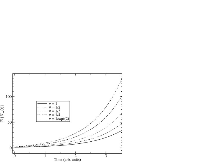
Figure 1: Mean number of individuals at time $t$ for various values of $\nu$.

An interesting representation of (93) following from (78) gives that

$$\mathbb{E}N_{\nu}(t)=\int_{0}^{\infty}\mathrm{e}^{\lambda s}\operatorname{Pr}\{T_{2\nu}(t)\in\mathrm{d}s\}=\int_{0}^{\infty}\mathbb{E}N(s)\operatorname{Pr}\{T_{2\nu}(t)\in\mathrm{d}s\}.$$ (95)

The expansion of the population subject to the law of the fractional birth process is increasingly rapid as the order of fractionality $\nu$ decreases. This is shown in Figure 1 and this behavior is due to the increasing structure of the gamma function for $\nu>0$ appearing in the Mittag–Leffler function $E_{\nu,1}$. This qualitative feature of the process being investigated here shows that it conveniently applies to explosively expanding populations.

Remark 3.0.

By twice deriving (91) with respect to $u$, we obtain the fractional equation for the second-order factorial moment

$$\mathbb{E}\bigl{\{}N_{\nu}(t)\bigl{(}N_{\nu}(t)-1\bigr{)}\bigr{\}}=g_{\nu}(t),$$ (96)

that is,

$$\cases{{\displaystyle\frac{\partial^{\nu}}{\partial t^{\nu}}}g_{\nu}(t)=2\lambda g_{\nu}(t)+2\lambda\mathbb{E}N_{\nu}(t),&\quad$0<\nu\leq 1,$\vspace*{2pt}\cr g_{\nu}(0)=0.&}$$ (97)

The Laplace transform of the solution to (97) is

$$H_{\nu}(t) = \int_{0}^{\infty}\mathrm{e}^{-\mu t}g_{\nu}(t)\,\mathrm{d}t=\frac{2\lambda\mu^{\nu-1}}{(\mu^{\nu}-\lambda)(\mu^{\nu}-2\lambda)}$$

$$= 2\mu^{\nu-1}\biggl{\{}\frac{1}{\mu^{\nu}-2\lambda}-\frac{1}{\mu^{\nu}-\lambda}\biggr{\}}.$$

The inverse Laplace transform of (11) is

$$\mathbb{E}\bigl{\{}N_{\nu}(t)\bigl{(}N_{\nu}(t)-1\bigr{)}\bigr{\}}=2E_{\nu,1}(2\lambda t^{\nu})-2E_{\nu,1}(\lambda t^{\nu}).$$ (99)

It is now straightforward to obtain the variance from (99),

$$\operatorname{\mathbb{V}ar}N_{\nu}(t)=2E_{\nu,1}(2\lambda t^{\nu})-E_{\nu,1}(\lambda t^{\nu})-E_{\nu,1}^{2}(\lambda t^{\nu}).$$ (100)

For $\nu=1$, we retrieve from (100) the well-known expression of the variance of the linear birth process

$$\operatorname{\mathbb{V}ar}N_{1}(t)=\mathrm{e}^{\lambda t}(\mathrm{e}^{\lambda t}-1).$$ (101)

Remark 3.0.

If $X_{1},\ldots,X_{n}$ are i.i.d. random variables with common distribution $F(x)=\break\operatorname{Pr}(X<x)$, then we can write the following probability:

$$\operatorname{Pr}\bigl{\{}\max\bigl{(}X_{1},\ldots,X_{N_{\nu}(t)}\bigr{)}<x\bigr{\}}$$

$$\quad=\sum_{k=1}^{\infty}(\operatorname{Pr}\{X<x\})^{k}\operatorname{Pr}\{N_{\nu}(t)=k\}\qquad\mbox{(by (\ref{iteration}))}$$

(102)

$$\quad=\int_{0}^{\infty}G(F(x),s)\operatorname{Pr}\{T_{2\nu}(t)\in\mathrm{d}s\}$$

$$\quad=\int_{0}^{\infty}\frac{F(x)\mathrm{e}^{-\lambda s}}{1-F(x)(1-\mathrm{e}^{-\lambda s})}\operatorname{Pr}\{T_{2\nu}(t)\in\,\mathrm{d}s\}.$$

Analogously, we have that

$$\operatorname{Pr}\bigl{\{}\min\bigl{(}X_{1},\ldots,X_{N_{\nu}(t)}\bigr{)}>x\bigr{\}}$$

(103)

$$\quad=\int_{0}^{\infty}\frac{(1-F(x))\mathrm{e}^{-\lambda s}}{1-(1-F(x))(1-\mathrm{e}^{-\lambda s})}\operatorname{Pr}\{T_{2\nu}(t)\in\,\mathrm{d}s\}.$$

Remark 3.0.

If the initial number of components of the population is $n_{0}$, then the p.g.f. becomes

$$\mathbb{E}\bigl{(}u^{N_{\nu}(t)}|N_{\nu}(0)=n_{0}\bigr{)}$$

(104)

$$\quad=\sum_{k=0}^{\infty}u^{k+n_{0}}\int_{0}^{\infty}\mathrm{e}^{-\lambda zn_{0}}\pmatrix{{n_{0}+k-1}\cr{k}}(1-\mathrm{e}^{-\lambda z})^{k}\operatorname{Pr}\{T_{2\nu}(t)\in\,\mathrm{d}z\}.$$

From (13), we can extract the distribution of the population size at time $t$ as

$$\operatorname{Pr}\{N_{\nu}(t)=k+n_{0}|N_{\nu}(0)=n_{0}\}$$

(105)

$$\quad=\pmatrix{{n_{0}+k-1}\cr{k}}\int_{0}^{\infty}\mathrm{e}^{-\lambda zn_{0}}(1-\mathrm{e}^{-\lambda z})^{k}\operatorname{Pr}\{T_{2\nu}(t)\in\,\mathrm{d}z\},\qquad k\geq 0.$$

If we write $k+n_{0}=k^{\prime}$, then we can rewrite (13) as

$$\operatorname{Pr}\{N_{\nu}(t)=k^{\prime}|N_{\nu}(0)=n_{0}\}$$

(106)

$$\quad=\pmatrix{{k^{\prime}-1}\cr{k^{\prime}-n_{0}}}\int_{0}^{\infty}\mathrm{e}^{-\lambda zn_{0}}(1-\mathrm{e}^{-\lambda z})^{k^{\prime}-n_{0}}\operatorname{Pr}\{T_{2\nu}(t)\in\,\mathrm{d}z\},\qquad k^{\prime}\geq n_{0},$$

where $k^{\prime}$ is the number of individuals in the population at time $t$. For $n_{0}=1$, formulas (13), (13) coincide with (4). The random time $T_{2\nu}(t)$, $t>0$, appearing in (13) and (13) has a distribution which is related to the fractional equation

$$\frac{\partial^{2\nu}u}{\partial t^{2\nu}}=\frac{\partial^{2}u}{\partial z^{2}},\qquad 0<\nu\leq 1.$$ (107)

It is possible to slightly change the structure of formulas (13) and (13) by means of the transformation $\lambda z=y$ so that the distribution of $T_{2\nu}(t)$ becomes related to the equation

$$\frac{\partial^{2\nu}u}{\partial t^{2\nu}}=\lambda^{2}\frac{\partial^{2}u}{\partial y^{2}},\qquad 0<\nu\leq 1,$$ (108)

where (52) shows the connection between the diffusion coefficient in (108) and the birth rate.

Remark 3.0.

If we assume that the initial number of individuals in the population is $N_{\nu}(0)=n_{0}$, then we can generalize the result (4) offering a representation of the distribution of $N_{\nu}(t)$ alternative to (13). If we take the Laplace transform of (13), then we have that

$$\int_{0}^{\infty}\mathrm{e}^{-\mu t}\operatorname{Pr}\{N_{\nu}(t)=k+n_{0}|N_{\nu}(0)=n_{0}\}\,\mathrm{d}t$$

$$\quad=\int_{0}^{\infty}\pmatrix{{n_{0}+k-1}\cr{k}}\int_{0}^{\infty}\mathrm{e}^{-\lambda zn_{0}}(1-\mathrm{e}^{-\lambda z})^{k}\operatorname{Pr}\{T_{2\nu}(t)\in\,\mathrm{d}z\}\,\mathrm{d}t\qquad\operatorname{(by(\ref{lapl-trans-folded}))}$$

$$\quad=\int_{0}^{\infty}\pmatrix{{n_{0}+k-1}\cr{k}}\mathrm{e}^{-\lambda zn_{0}}(1-\mathrm{e}^{-\lambda z})^{k}\mu^{\nu-1}\mathrm{e}^{-\mu^{\nu}z}\,\mathrm{d}z$$

(109)

$$\quad=\pmatrix{{n_{0}+k-1}\cr{k}}\mu^{\nu-1}\int_{0}^{\infty}\mathrm{e}^{-z(\lambda n_{0}+\mu^{\nu})}(1-\mathrm{e}^{-\lambda z})^{k}\,\mathrm{d}z$$

$$\quad=\pmatrix{{n_{0}+k-1}\cr{k}}\mu^{\nu-1}\sum_{r=0}^{k}\pmatrix{{k}\cr{r}}(-1)^{r}\int_{0}^{\infty}\mathrm{e}^{-z(\lambda n_{0}+\lambda r+\mu^{\nu})}\,\mathrm{d}z$$

$$\quad=\pmatrix{{n_{0}+k-1}\cr{k}}\mu^{\nu-1}\sum_{r=0}^{k}\pmatrix{{k}\cr{r}}(-1)^{r}\frac{1}{\lambda(n_{0}+r)+\mu^{\nu}}.$$

By taking the inverse Laplace transform of (14), we have that

$$\operatorname{Pr}\{N_{\nu}(t)=k+n_{0}|N_{\nu}(0)=n_{0}\}$$

(110)

$$\quad=\pmatrix{{n_{0}+k-1}\cr{k}}\sum_{r=0}^{k}\pmatrix{{k}\cr{r}}(-1)^{r}E_{\nu,1}\bigl{(}-(n_{0}+r)\lambda t^{\nu}\bigr{)}.$$

From (14), we can infer the interesting information

$$\operatorname{Pr}\{N_{\nu}(\mathrm{d}t)=n_{0}+1|N_{\nu}(0)=n_{0}\}$$

$$\quad=n_{0}\sum_{r=0}^{1}\pmatrix{{1}\cr{r}}(-1)^{r}E_{\nu,1}\bigl{(}-(n_{0}+r)\lambda(\mathrm{d}t)^{\nu}\bigr{)}$$ (111)

$$\quad=n_{0}\bigl{[}E_{\nu,1}\bigl{(}-n_{0}\lambda(\mathrm{d}t)^{\nu}\bigr{)}-E_{\nu,1}\bigl{(}-\lambda(n_{0}+1)(\mathrm{d}t)^{\nu}\bigr{)}\bigr{]}\sim n_{0}\frac{\lambda(\mathrm{d}t)^{\nu}}{\Gamma(\nu+1)}$$

by writing only the lower order terms. This shows that the probability of a new offspring at the beginning of the process is proportional to $(\mathrm{d}t)^{\nu}$ and to the initial number of progenitors. From our point of view, this is the most important qualitative feature of our results since it makes explicit the dependence on the order $\nu$ of the fractional birth process.

Theorem 15

The Laplace transform of the probability generating function $G_{\nu}(t,u)$ of the fractional linear birth process has the form

$$H_{\nu}(\mu,u)=\int_{0}^{\infty}\mathrm{e}^{-\mu t}G_{\nu}(t,u)\,\mathrm{d}t=\frac{u\mu^{\nu-1}}{\lambda}\int_{0}^{1}\frac{(1-x)^{{\mu^{\nu}}/{\lambda}}}{1-xu}\,\mathrm{d}x,\qquad\mbox{$0<u<1$, $\mu>0$}.$$ (112)

Proof.

We saw above that the function $G_{\nu}$ solves the Cauchy problem

$$\cases{{\displaystyle\frac{\partial^{\nu}G_{\nu}}{\partial t^{\nu}}}=\lambda u(u-1){\displaystyle\frac{\partial G_{\nu}}{\partial u}},&\quad$0<\nu\leq 1,$\vspace*{2pt}\cr G_{\nu}(u,0)=u.&}$$ (113)

By taking the Laplace transform of (113), we have that

$$\mu^{\nu}H_{\nu}-\mu^{\nu-1}u=\lambda u(u-1)\frac{\partial H_{\nu}}{\partial u}.$$ (114)

By inserting (112) into (114) and performing some integrations by parts, we have that

$$\frac{u\mu^{2\nu-1}}{\lambda}\int_{0}^{1}\frac{(1-x)^{{\mu^{\nu}}/{\lambda}}}{1-xu}\,\mathrm{d}x-u\mu^{\nu-1}$$

$$\quad=\lambda u(u-1)\biggl{[}\frac{\mu^{\nu-1}}{\lambda}\int_{0}^{1}\frac{(1-x)^{{\mu^{\nu}}/{\lambda}}}{1-xu}\,\mathrm{d}x+\frac{u\mu^{\nu-1}}{\lambda}\int_{0}^{1}\frac{(1-x)^{{\mu^{\nu}}/{\lambda}}x}{(1-xu)^{2}}\,\mathrm{d}x\biggr{]}$$

$$\quad=\lambda u(u-1)\biggl{[}\frac{\mu^{\nu-1}}{\lambda}\int_{0}^{1}\frac{(1-x)^{{\mu^{\nu}}/{\lambda}}}{1-xu}\,\mathrm{d}x+\frac{\mu^{\nu-1}}{\lambda}\frac{x(1-x)^{{\mu^{\nu}}/{\lambda}}}{1-xu}\bigg{|}_{x=0}^{x=1}$$

(115)

$$\quad\phantom{=\lambda u(u-1)\biggl{[}}{}-\frac{\mu^{\nu-1}}{\lambda}\int_{0}^{1}\frac{(1-x)^{{\mu^{\nu}}/{\lambda}}}{(1-xu)}\,\mathrm{d}x+\frac{\mu^{2\nu-1}}{\lambda^{2}}\int_{0}^{1}\frac{x(1-x)^{{\mu^{\nu}}/{\lambda}-1}}{(1-xu)}\,\mathrm{d}x\biggr{]}\qquad$$

$$\quad=\frac{u(u-1)\mu^{2\nu-1}}{\lambda}\int_{0}^{1}\frac{x(1-x)^{{\mu^{\nu}}/{\lambda}-1}}{(1-xu)}\,\mathrm{d}x$$

$$\quad=-u\mu^{\nu-1}+\frac{u\mu^{2\nu-1}}{\lambda}\int_{0}^{1}\frac{(1-x)^{{\mu^{\nu}}/{\lambda}}}{(1-xu)}\,\mathrm{d}x,$$

and this concludes the proof of Theorem 15. ∎

Remark 3.0.

We note that $H_{\nu}(\mu,u)|_{u=1}=1/\mu$ because $G_{\nu}(t,1)=1$. Furthermore,

$$\frac{\partial H_{\nu}(\mu,u)}{\partial u}\bigg{|}_{u=1}=\frac{\mu^{\nu-1}}{\mu^{\nu}-\lambda}=\int_{0}^{\infty}\mathrm{e}^{-\mu t}E_{\nu,1}(\lambda t^{\nu})\,\mathrm{d}t,$$ (116)

which accords well with (93).

References

• [1] Bartlett, M.S. (1978). An Introduction to Stochastic Processes, with Special Reference to Methods and Applications, 3rd ed. Cambridge: Cambridge Univ. Press. MR0475536
• [2] Beghin, L. and Orsingher, E. (2009). Fractional Poisson processes and related planar random motions. Electron. J. Probab. 14 1970–1827. MR2535014
• [3] Cahoy, D.O. (2007). Fractional Poisson processes in terms of alpha-stable densities. Ph.D. thesis.
• [4] Feller, W. (1968). An Introduction to Probability Theory and Its Applications, Volume 1, 3rd ed. New York: Wiley. MR0228020
• [5] Gikhman, I.I. and Skorokhod, A.V. (1996). Introduction to the Theory of Random Processes. New York: Dover Publications. MR1435501
• [6] Gradshteyn, I.S. and Ryzhik, I.M. (1980). Table of Integrals, Series, and Products. New York: Academic Press. MR0582453
• [7] Jumarie, G. (2001). Fractional master equation: Non-standard analysis and Liouville–Riemann derivative. Chaos Solitons Fractals 12 2577–2587. MR1851079
• [8] Kirschenhofer, P. (1996). A note on alternating sums. Electron. J. Combin. 3 1–10. MR1392492
• [9] Laskin, N. (2003). Fractional Poisson process. Commun. Nonlinear Sci. Numer. Simul. 8 201–213. MR2007003
• [10] Orsingher, E. and Beghin, L. (2004). Time-fractional telegraph equations and telegraph processes with Brownian time. Probab. Theory Related Fields 128 141–160. MR2027298
• [11] Orsingher, E. and Beghin, L. (2009). Fractional diffusion equations and processes with randomly-varying time. Ann. Probab. 37 206–249. MR2489164
• [12] Podlubny, I. (1999). Fractional Differential Equations. San Diego: Academic Press. MR1658022
• [13] Repin, O.N. and Saichev, A.I. (2000). Fractional Poisson law. Radiophys. and Quantum Electronics 43 738–741. MR1910034
• [14] Samorodnitsky, G. and Taqqu, M.S. (1994). Stable Non-Gaussian Random Processes: Stochastic Models with Infinite Variance. New York: Chapman and Hall. MR1280932
• [15] Uchaikin, V.V. and Sibatov, R.T. (2008). A fractional Poisson process in a model of dispersive charge transport in semiconductors. Russian J. Numer. Anal. Math. Modelling 23 283–297. MR2414873
• [16] Uchaikin, V.V., Cahoy, D.O. and Sibatov, R.T. (2008). Fractional processes: From Poisson to branching one. Int. J. Bifurcation Chaos 18 2717–2725. MR2479327
• [17] Wang, X.-T. and Wen, Z.-X. (2003). Poisson fractional processes. Chaos Solitons Fractals 18 169–177. MR1984556
• [18] Wang, X.-T., Wen, Z.-X. and Zhang, S.-Y. (2006). Fractional Poisson process (II). Chaos Solitons Fractals 28 143–147. MR2174587
• [19] Wang, X.-T., Zhang, S.-Y. and Fan, S. (2007). Nonhomogeneous fractional Poisson processes. Chaos Solitons Fractals 31 236–241. MR2263284