Rotational Doppler Effect in Magnetic Resonance

Abstract

We compute the shift in the frequency of the spin resonance in a solid that rotates in the field of a circularly polarized electromagnetic wave. Electron spin resonance, nuclear magnetic resonance, and ferromagnetic resonance are considered. We show that contrary to the case of the rotating LC circuit, the shift in the frequency of the spin resonance has strong dependence on the symmetry of the receiver. The shift due to rotation occurs only when rotational symmetry is broken by the anisotropy of the gyromagnetic tensor, by the shape of the body, or by magnetocrystalline anisotropy. General expressions for the resonance frequency and power absorption are derived and implications for experiment are discussed.

I Introduction

The term Rotational Doppler Effect (RDE) is used to describe a frequency shift encountered by a receiver of electromagnetic radiation when either the receiver or the source of the radiation are rotating. The effect is illustrated in Fig. 1. The frequency of the wave, $\omega=2\pi f$, measured at a given point in space, corresponds to the angular velocity of the rotation of the electric (magnetic) field due to the wave. If the receiver is rotating mechanically at an angular velocity $\Omega$ about the axis parallel to the wave vector ${\bf k}$, than the frequency of the wave perceived by the receiver equals

$$\omega^{\prime}=\omega\pm\Omega\,.$$ (1)

The sign, plus or minus, depends on the helicity of the wave and the direction of the rotation of the receiver.

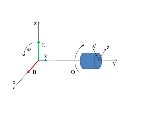
Figure 1: Color online: Rotational Doppler effect. The frequency $\omega$ of the circularly polarized electromagnetic wave $(\omega,{\bf k})$ is the angular velocity of the rotation of the electric (magnetic) field due to the wave at a given point in space. The rotation of the receiver at an angular velocity $\Omega$, depending on the direction of the rotation and the helicity of the wave, adds or subtracts $\Omega$ to the frequency of the wave $\omega$, rendering $\omega^{\prime}=\omega\pm\Omega$ in the coordinate frame of the receiver.

The RDE is less commonly known than the conventional Doppler effect. One reason is that it is more difficult to observe. Mössbauer technique provides the most sensitive method for the study of the frequency shift due to the conventional Doppler effect, $\delta\omega=(v/c)\omega$ for $v\ll c$. The limiting velocity has been a fraction of a millimeter per second and is due to the finite very small linewidth of gamma radiation, $\delta\omega/\omega\sim 10^{-13}-10^{-12}$. Such a small linewidth has even permitted observation of the transverse Doppler effect Hay1960-Champeney1961-Kundig1963 ; Kholmetskii2008-Kholmetskii2009 by performing Mössbauer experiment on a rotating platform. This effect, not to be confused with the RDE, consists of the frequency shift $\delta\omega/\omega=-v^{2}/(2c^{2})$ due to the relativistic time dilation for a receiver moving tangentially with respect to the source of the radiation. It is easy to see, however, that the frequency shift as little as $\Omega/\omega\sim 10^{-13}-10^{-12}$ due the RDE would require angular velocity of the emitter or the receiver in the Mössbauer experiment on the order of a few MHz or even a few tens of MHz. The latter is still one-two orders of magnitude greater than the angular velocities of high-speed rotors used for magic angle spinning in NMR applications.

The RDE frequency shift caused by a rotating plate inserted into a beam of circularly polarized light was reported in Refs. Garetz1979, ; Simon1988, ; Bretaneker1990, ; Basstiy2002, ; Chen2008, . The RDE was predicted for rotating light beams Nienhuis1996 and subsequently observed using millimeter waves Courtial1998 as well as in the optical range Barreiro2006 (see Ref. Padgett2006, for review). In solid state experiments the RDE has proved surprisingly elusive. Frequencies of the ferromagnetic resonance (FMR) are typically in the GHz range or higher, which is far above achievable angular velocities of mechanical rotation of macroscopic magnets. However, small magnetic particles in beams Xu-2005 or in nanopores FR may rotate very fast. Eq. (1) was recently applied to the analysis of the observed anomalies in the FMR data on rotating nanoparticles FR . The RDE may be especially important for the NMR technology that uses rapidly spinning samples. Frequency shifts of the quadrupole line in the nuclear magnetic resonance (NMR) experiment with a rotating sample were reported in Ref. Tycko1987, and analyzed in terms of Berry phase Berry . It was never fully explained, however, why such shifts do not persist in the NMR experiments in which the angular velocity of the magic-angle-spinning rotor with the sample often exceeds the linewidth by an order of magnitude. Some hint to answering this question can be found in Ref. BB-1997, that studied the effect of the rotation on radiation at the atomic level. The authors of this work correctly argued that the RDE can only be seen in the radiation of atoms and molecules placed in the environment that destroys rotational symmetry.

Situation depicted in Fig. 1 rather obviously leads to the frequency shift by $\Omega$ when the emitter and the receiver are based upon LC circuits. This has been tested by the GPS for the case of a receiving antenna making as little as $8$ revolutions per second as compared to the carrier frequency of the electromagnetic waves in the GHz range Ashby . Eq. (1) has been also applied to the explanation of the frequency shift encountered by NASA in the communications with Pioneer spacecrafts Mashhoon-Pioneer . One essential difference between conventional and rotational Doppler effects is that the first refers to the inertial systems while the second occurs in the non-inertial systems. This prompted works that considered RDE in the context of nonlocal quantum mechanics in the accelerated frame of reference Mashhoon-Relativity . Relativity (or Galilean invariance for $v\ll c$) makes the conventional Doppler effect quite universal. As we shall see below, such a universality should not be expected for the RDE. Indeed, the argument behind the RDE is based upon perception of a circularly polarized wave by a rotating observer. Through the Larmor theorem LL-FT the mechanical rotation of the system of charges is equivalent to the magnetic field. Consequently, when making the argument, one has to check whether the resonant frequency of the receiver is affected by the magnetic field. Resonant frequencies of LC circuits are known to be insensitive to the magnetic fields, thus making the argument rather solid. On the contrary, the frequency of the receiver based upon magnetic resonance would be sensitive to the fictitious magnetic field due to rotation, thus making the argument incomplete.

In this paper we develop a rigorous theory of the RDE for magnetic resonance. We show that the frequency shift due to rotation is always different from $\Omega$. Broken rotational symmetry is required for the shift to have a non-zero value, in which case the magnetic resonance splits into two lines separated by $2\Omega$. For the electron spin resonance (ESR) violation of the rotational symmetry would naturally arise from the anisotropy of the gyromagnetic tensor. In a solid state NMR experiment with a rotating sample, violation of symmetry would be more common in the presence of the magnetic order that provides anisotropy of the hyperfine interaction. For a ferromagnetic resonance (FMR) the asymmetry comes from the shape of the sample and from magnetocrystalline anisotropy. The paper is organized as follows. The physics of spin-rotation coupling is reviewed in Section II. Frequency shift of the ESR in a rotating crystal with anisotropic gyromagnetic tensor is computed in Section III. The effect of rotation on the NMR spectra is discussed in Section IV. FMR in a rotating sample is studied in Section V. Power absorption by the rotating magnet is considered in Section VI. Section VII contains some suggestions for experiment and discussion of possible application of the RDE in solid state physics.

II Spin-rotation coupling

In classical mechanics the Hamiltonian of the system in a rotating coordinate frame is given by LL-M

$${\cal{H}}^{\prime}=\cal{H}-{\bf L}\cdot{\bf\Omega}\,.$$ (2)

Here $\cal{H}$ is the Hamiltonian at $\Omega=0$ and ${\bf L}$ is the mechanical angular momentum of the system. For a system of charges one can write

$${\bf L}=\frac{\bf M}{\gamma}\,,$$ (3)

where ${\bf M}$ is the magnetic moment and $\gamma$ is the gyromagnetic ratio. Eq. (2) then becomes equivalent to the Hamiltonian,

$${\cal{H}}^{\prime}=\cal{H}-{\bf M}\cdot{\bf B}\,,$$ (4)

in the fictitious magnetic field,

$${\bf B}=\frac{\bf\Omega}{\gamma}\,,$$ (5)

which is the statement of the Larmor theorem LL-FT .

Neither classical mechanics nor classical field theory deals with the concept of a spin. The question then arises whether Eq. (2) should contain spin ${\bf S}$ alongside with the orbital angular momentum ${\bf L}$. Eq. (4) hints that since the magnetic moment can be of spin origin this should be the case. Also it is known from relativistic physics that the generator of rotations is

$${\bf J}={\bf L}+{\bf S}\,.$$ (6)

It should be, therefore, naturally expected that in the presence of a spin Eq. (2) should be generalized as

$${\cal{H}}^{\prime}=\cal{H}-({\bf L}+{\bf S})\cdot{\bf\Omega}\,.$$ (7)

In quantum theory this relation can be rigorously derived in the following way. Rotation by an angle ${\bm{\phi}}$ transforms the Hamiltonian of an isolated system into QM

$$\hat{\cal{H}}^{\prime}=\exp\left[\frac{i}{\hbar}(\mathbf{L}+\mathbf{S})\cdot{\bm{\phi}}\right]\hat{\cal{H}}\exp\left[-\frac{i}{\hbar}(\mathbf{L}+\mathbf{S})\cdot{\bm{\phi}}\right]\,.$$ (8)

To the first order on a small rotation ${\bm{\phi}}$ one obtains

$$\hat{\cal{H}}^{\prime}=\hat{\cal{H}}-\frac{i}{\hbar}(\mathbf{L}+\mathbf{S})\cdot[\hat{\cal{H}},{\bm{\phi}}]\,,$$ (9)

where we have taken into account that for an isolated system ${\bf J}$ is conserved, that is ${\bf L}+{\bf S}$ commutes with $\hat{\cal{H}}$. This equation becomes Eq. (7) if one takes into account the quantum-mechanical relation

$${\bf\Omega}=\frac{d{\bm{\phi}}}{dt}=\frac{i}{\hbar}[\hat{\cal{H}},{\bm{\phi}}]$$ (10)

and replaces operator ${\bf\Omega}$ by its classical expectation value. For an electron Eq. (7) can be also formally derived as a non-relativistic limit of the Dirac equation written in the metric of the rotating coordinate frame Hehl1990 . The answer for the corresponding Schrödinger equation reads

$$i\hbar\frac{\partial\Psi}{\partial t}=\hat{\cal{H}}^{\prime}\Psi\,,\quad\hat{\cal{H}}^{\prime}=\frac{{\hat{\bf p}}^{2}}{2m}-\left({\bf r}\times\hat{\bf p}+\frac{1}{2}\hbar\hat{\bm{\sigma}}\right)\cdot{\bf\Omega}\,,$$ (11)

where ${\bf r}$ and ${\bf p}=-i\hbar{\bm{\nabla}}$ are the radius-vector and the linear momentum of the electron, respectively, and ${\sigma}_{x,y,z}$ are Pauli matrices.

There has been some confusion in literature regarding the term $-{\bf S}\cdot{\bf\Omega}$ in the Hamiltonian of the body studied in the coordinate frame that rotates together with the body EC-PRL1994 ; Villain ; CGS . To elucidate the physical meaning of this term, let us consider the resulting equation of motion for a classical spin-vector CT

$$\frac{d{\bf S}}{dt}=-{\bf S}\times\frac{\delta{\cal{H}}^{\prime}}{\delta{\bf S}}\,.$$ (12)

If $\cal{H}$ does not depend on spin, then the spin cannot be affected in any way by the rotation of the body. In this case ${\delta{\cal{H}}^{\prime}}/{\delta{\bf S}}=-{\bf\Omega}$ and Eq. (12) simply describes the precession of ${\bf S}$ about ${\bf\Omega}$:

$$\frac{d{\bf S}}{dt}={\bf S}\times{\bf\Omega}\,.$$ (13)

It shows how a constant vector ${\bf S}$ (or any other vector to this matter) is viewed by an observer rotating at an angular velocity ${\bf\Omega}$. This has nothing to do with the spin-orbit or any other interaction. Such interactions should be accounted for in the $\hat{\cal{H}}$ part of the Hamiltonian $\hat{\cal{H}}^{\prime}$. The effect of rotations on various magnetic resonances is considered in the next sections.

III Frequency Shift of the Electron Spin Resonance Due to Rotation

In this Section we consider an electron in a rotating crystal or in a rotating quantum dot characterized by the anisotropic gyromagnetic tensor, $g_{ij}$. The effect of local rotations due to transverse phonons on the width of the ESR has been studied in Ref. CCG, . Here we are interested in the effect of the global rotation on the ESR frequency. To deal with the stationary states we shall assume that the axis of rotation ${\bf\Omega}$ is parallel to the applied magnetic field ${\bf B}$ and will compute the energy levels of the electron as measured by the observer rotating together with the system. In the rotating frame the spin Hamiltonian of the electron is

$$\hat{\cal{H}}^{\prime}=\frac{1}{2}\mu_{B}\,g_{ij}\,{\sigma}_{i}B_{j}-\frac{1}{2}\hbar{\bm{\sigma}}\cdot{\bf\Omega}\,.\vspace{1mm}$$ (14)

Positive sign of the first (Zeeman) term is due to the negative gyromagnetic ratio $\gamma$ for the electron ($\mu_{B}=\hbar|\gamma|$ being the Bohr magneton).

The geometry of the problem is illustrated in Fig. 2. In the rotating frame the solid matrix containing the electron is stationary. It is convenient to choose the coordinate axes of that matrix along the principal axes of the tensor $g_{ij}$. Then $g_{ij}$ is diagonal,

$$g_{ij}=g_{i}\delta_{ij},$$ (15)

represented by three numbers, $g_{x}$, $g_{y}$, and $g_{z}$ that can be directly measured when the system is at rest. Eq. (14) then becomes

$$\hat{\cal{H}}^{\prime} = \frac{1}{2}\left[(\mu_{B}\,g_{x}B_{x}-\hbar\Omega_{x})\,{\sigma}_{x}+(\mu_{B}\,g_{y}B_{y}-\hbar\Omega_{y})\,{\sigma}_{y}\right.$$ (16)

$$+ \left.(\mu_{B}\,g_{z}B_{z}-\hbar\Omega_{z})\,{\sigma}_{z}\right]\,.$$

Diagonalization of this Hamiltonian with the account of the fact that ${\bf\Omega}$ was chosen parallel to ${\bf B}$ gives the following energy levels of $\hat{\cal{H}}^{\prime}$:

$$E_{\pm}=\pm\frac{1}{2}\mu_{B}B\left[\sum_{i=x,y,z}\left(g_{i}-\frac{\hbar\Omega}{\mu_{B}B}\right)^{2}n_{i}^{2}\right]^{1/2}\,$$ (17)

Here ${\bf n}$ is the unit vector in the direction of the axis of rotation,

$${\bf n}=\frac{\bf\Omega}{\Omega}=\frac{\bf B}{B}\,.$$ (18)

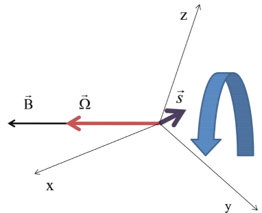
Figure 2: Color online: Spin in the magnetic field parallel to the rotation axis of the crystal. The rotating coordinate axes $x,y,z$ are chosen along the principal axes of the gyromagnetic tensor.

In practice, the angular velocity of the mechanical rotation will always be sufficiently small to provide the condition $\hbar\Omega\ll\mu_{B}B$. Contribution of the rotation to the ESR frequency in the rotating frame,

$$\hbar\omega^{\prime}_{ESR}={E_{+}-E_{-}}\,,$$ (19)

will, therefore, be small compared to the ESR frequency

$$\hbar\omega_{ESR}={\mu_{B}}B(g_{x}^{2}n_{x}^{2}+g_{y}^{2}n_{y}^{2}+g_{z}^{2}n_{z}^{2})^{1/2}$$ (20)

unperturbed by rotation. Expanding Eq. (17) to the first order in $\Omega$ one obtains

$$\omega^{\prime}_{ESR}=\omega_{ESR}-\kappa\Omega\,,$$ (21)

$$\kappa=\frac{g_{x}n_{x}^{2}+g_{y}n_{y}^{2}+g_{z}n_{z}^{2}}{\sqrt{g_{x}^{2}n_{x}^{2}+g_{y}^{2}n_{y}^{2}+g_{z}^{2}n_{z}^{2}}}\,.$$ (22)

Here $\Omega$ can be positive or negative depending on the direction of rotation.

Few observations are in order. Firstly, according to Eq. (22), the frequency shift for the observer rotating together with the sample containing the electron is never zero. Secondly, when the rotation is about one of the principal axes of the gyromagnetic tensor, Eq. (22) gives $\kappa=1$, so that the frequency shift for the rotating observer is exactly $\Omega$. The ESR occurs when the frequency $\omega^{\prime}$ of the circularly polarized electromagnetic wave perceived by the rotating observer and given by Eq. (1) coincides with $\omega^{\prime}_{ESR}$. If the rotation is about one of the principal axes of $g_{ij}$, then $\kappa=1$ and the angular velocity $\Omega$ cancels exactly from the equation $\omega^{\prime}=\omega_{ESR}^{\prime}$ for the polarization of the wave that corresponds to $\omega^{\prime}=\omega-\Omega$, thus, resulting in no RDE frequency shift for an experimentalist working in the laboratory frame. For the opposite polarization of the wave, corresponding to $\omega^{\prime}=\omega+\Omega$, the shift in the rotationally invariant case formally equals $2\Omega$. However, such photons would have their spin projection in the direction opposite to the one necessary to produce the spin transition. They can be absorbed only when the rotational symmetry is broken so that the electron spin in the direction of the wave vector is no longer a good quantum number (see Section VI).

IV Frequency Shift of the Nuclear Magnetic Resonance Due to Rotation

Let us consider a nuclear spin ${\bf I}$ in the magnetic field parallel to the axis of rotation of the sample. It is clear from the previous section that the mechanical rotation combined with the rotationally invariant Zeeman interaction of the nuclear magnetic moment with the field,

$$\hat{\cal{H}}^{\prime}=-\gamma_{n}g_{n}{\bf I}\cdot{\bf B}-{\bf I}\cdot{\bf\Omega}\,,$$ (23)

(with $\gamma_{n}>0$ and $g_{n}$ being nuclear gyromagnetic ratio and gyromagnetic factor, respectively) are not sufficient to produce the RDE. Isotropic hyperfine interaction with an atomic spin ${\bf S}$ of the form $-A{\bf I}\cdot{\bf S}$ would not change this either. However, an anisotropic hyperfine interaction,

$$\hat{\cal{H}}_{hf}=-A_{ij}I_{i}S_{j}\,,$$ (24)

in principle, can do the job. If there is a ferromagnetic order in the solid, then ${\bf S}$ develops a non-zero average, $\langle{\bf S}\rangle$. Replacing $S_{j}$ in Eq. (24) with $\langle S_{j}\rangle$ and adding the hyperfine interaction to Eq. (23), one obtains

$$\hat{\cal{H}}^{\prime}=-\gamma_{n}g_{n}{\bf I}\cdot{\bf B}-A_{ij}I_{i}\langle S_{j}\rangle-{\bf I}\cdot{\bf\Omega}\,.$$ (25)

To work with the stationary energy states in the rotating frame, we shall assume that all three vectors ${\bf B}$, $\langle{\bf S}\rangle$, and ${\bf\Omega}$ are parallel to each other. Let us study the case of $I=1/2$. Choosing the coordinate axes along the principal axes of tensor $A_{ij}=A_{i}\delta_{ij}$, it is easy to see that Eq. (25) is equivalent to the Zeeman Hamiltonian,

$$\hat{\cal{H}}^{\prime}=-\frac{1}{2}\mu_{n}\left[g_{x}^{eff}\sigma_{x}B_{x}+g_{y}^{eff}\sigma_{y}B_{y}+g_{z}^{eff}\sigma_{z}B_{z}\right]$$ (26)

with an effective gyromagnetic tensor whose principal values are given by ($i=x,y,z$)

$$g_{i}^{eff}=g_{n}+\frac{B^{hf}_{i}}{B}+\frac{\hbar\Omega}{\mu_{n}B}\,,\vspace{1mm}$$ (27)

where we have introduced the nuclear magneton, $\mu_{n}=\hbar\gamma_{n}$, and the hyperfine field, ${\bf B}^{hf}$, with components

$$B^{hf}_{i}=\frac{\hbar A_{i}|\langle{\bf S}\rangle|}{\mu_{n}}\,.$$ (28)

The energy levels of the Hamiltonian (26) are

$$E_{\pm}=\pm\frac{1}{2}\mu_{n}B\left[\sum_{i=x,y,z}\left(g_{i}^{eff}\right)^{2}n_{i}^{2}\right]^{1/2}\,,$$ (29)

where ${\bf n}={\bf B}/{B}$.

Let us consider the case of small $\Omega$. Making the series expansion of Eq. (29) one obtains to the first order on $\Omega$

$$\omega^{\prime}_{NMR}=\frac{E_{+}-E_{-}}{\hbar}=\omega_{NMR}+\kappa\Omega$$ (30)

with $\kappa$ given by

$$\kappa=\frac{\sum_{i=x,y,z}\left(g_{n}+{B^{hf}_{i}}/{B}\right)n_{i}^{2}}{\sqrt{\sum_{i=x,y,z}\left(g_{n}+{B^{hf}_{i}}/{B}\right)^{2}n_{i}^{2}}}\,.$$ (31)

In the case of the isotropic hyperfine interaction, $B^{hf}_{x}=B^{hf}_{y}=B^{hf}_{z}$ (that is, $A_{x}=A_{y}=A_{z}$), Eq. (31) gives $\kappa=1$. Same situation occurs when the direction of the field and the axis of rotation coincide with one of the principal axes of the tensor of hyperfine interactions. For arbitrary rotations Eq. (31) gives $\kappa\rightarrow 1$ when $B\gg B^{hf}$, making the frequency shift defined by $\omega^{\prime}=\omega^{\prime}_{NMR}$ negligible for the polarization ($\omega^{\prime}=\omega+\Omega$) that is predominantly absorbed due to the selection rule. Is is likely, therefore, that a significant RDE in the NMR can be observed only in magnetically ordered materials, in the field comparable or less than the hyperfine field, for rotations about axes that do not coincide with the symmetry axes of the crystal. If these conditions are satisfied, and the width of the resonance is not very large compared to $\Omega$, the NMR produced by linearly polarized waves would split into two lines of uneven intensity separated by $2\Omega$. In fact, the existing experimental techniques permit observation of this effect (see Section VII).

V Frequency Shift of the Ferromagnetic Resonance Due to Rotation

We now turn to the rotating ferromagnets. We begin with a simplest model of ferromagnetic resonance studied by Kittel Kittel . In this model one neglects the effects of magnetocrystalline anisotropy and considers a uniformly magnetized ferromagnetic ellipsoid in the external magnetic field ${\bf B}=\mu_{0}{\bf H}$ (with $\mu_{0}$ being the magnetic permeability of vacuum). The energy density of such a ferromagnet is determined by its Zeeman interaction with the external field and by magnetic dipole-dipole interactions inside the ferromagnet:

$${\cal{H}}=\mu_{0}\left[-{\bf M}\cdot{\bf H}+\frac{1}{2}N_{ij}M_{i}M_{j}\right]\,.$$ (32)

Here ${\bf M}$ is the magnetization and $N_{ij}$ is tensor of demagnetizing coefficients. The principal axes of $N_{ij}$ coincide with the axes of the ellipsoid. Choosing the coordinate axes along the principal axes and taking into account that for a ferromagnet

$${\bf M}^{2}=M_{x}^{2}+M_{y}^{2}+M_{z}^{2}=M_{0}^{2}$$ (33)

is a constant, one can rewrite Eq. (32) as

$${\cal{H}}=-\mu_{0}\left[{\bf M}\cdot{\bf H}+\frac{1}{2}(N_{x}-N_{z})M_{x}^{2}+\frac{1}{2}(N_{y}-N_{z})M_{y}^{2})\right],$$ (34)

where we have omitted unessential constant. For, e.g., an infinite circular cylinder $N_{x}=N_{y}=1/2,N_{z}=0$. In general, for an ellipsoid elongated along the $Z$-axis one has $N_{x}-N_{z}>0,N_{y}-N_{z}>0$, so that in the absence of the field the minimum of Eq. (34) corresponds to ${\bf M}$ in the $Z$-direction. This will still be true in the external field if the latter is applied in the $Z$-direction, which is the case we consider here. Note that a finite field is always needed to prevent the magnet from breaking into magnetic domains.

The FMR frequency, $\omega_{FMR}$, can be obtained from either classical or quantum mechanical treatment CT . Classically, it is the frequency of the precession of ${\bf M}$ about its equilibrium direction. To find $\omega_{FMR}$ one should linearize the equation,

$$\frac{d{\bf M}}{dt}=\gamma{\bf M}\times{\bf B}^{(eff)}\,,\quad{\bf B}^{(eff)}=-\frac{\delta\cal{H}}{\delta{\bf M}}\,,$$ (35)

around ${\bf M}=M_{0}{\bf e}_{z}$ ($\gamma<0$ being the gyromagnetic ratio). The answer reads Kittel

$$\omega_{FMR}=\sqrt{\omega_{x}\omega_{y}}\,,$$ (36)

where

$$\omega_{x} = |\gamma|[B+(N_{x}-N_{z})\mu_{0}M_{0}]$$

$$\omega_{y} = |\gamma|[B+(N_{y}-N_{z})\mu_{0}M_{0}]\,.$$ (37)

To study the RDE we should now solve the same problem in the coordinate frame rotating about the $Z$-axis at an angular velocity $\Omega$. In the presence of rotation the Hamiltonian becomes

$${\cal{H}}^{\prime}=\cal{H}-\frac{\bf M}{\gamma}\cdot{\bf\Omega}\,.$$ (38)

It is easy to see that for ${\bf\Omega}=\Omega{\bf e}_{z}$ this effectively adds ${\bf\Omega}/\gamma$ to the external field. Consequently, the FMR frequency in the rotating frame becomes

$$\omega_{FMR}^{\prime}=\sqrt{\omega^{\prime}_{x}\omega^{\prime}_{y}}$$ (39)

with

$$\omega^{\prime}_{x} = |\gamma|\left[B+\frac{\Omega}{\gamma}+(N_{x}-N_{z})\mu_{0}M_{0}\right]$$

$$\omega^{\prime}_{y} = |\gamma|\left[B+\frac{\Omega}{\gamma}+(N_{y}-N_{z})\mu_{0}M_{0}\right]\,.$$ (40)

Our immediate observation is that for a symmetric ellipsoid ($N_{x}=N_{y}$)

$$\omega_{FMR}^{\prime}=\omega_{FMR}-\Omega\,,$$ (41)

so that the RDE frequency shift determined by the equation $\omega^{\prime}=\omega-\Omega=\omega_{FMR}^{\prime}$ is exactly zero. For an asymmetric ellipsoid ($N_{x}\neq N_{y}$), expanding Eq. (39) into a series on $\Omega$ one obtains to the first order

$$\omega_{FMR}^{\prime}=\omega_{FMR}-\kappa\Omega\,,$$ (42)

with

$$\kappa=\frac{1}{2}\left(\sqrt{\frac{\omega_{x}}{\omega_{y}}}+\sqrt{\frac{\omega_{y}}{\omega_{x}}}\right)\,.$$ (43)

It is easy to see that $\kappa\geq 1$. At large fields, $B\gg\mu_{0}M_{0}$, equations (V) and (43) give $\kappa\rightarrow 1$, that is, no frequency shift due to the RDE. Sizable frequency shift of the FMR observed in the laboratory frame due to the rotation of the sample should occur only at $B$ not significantly exceeding $\mu_{0}M_{0}$ and only in a sample lacking the rotational symmetry.

One can easily generalize the above approach to take into account any type of the magnetocrystalline anisotropy. The formulas look especially simple in the case of the second-order anisotropy. Such anisotropy adds the term

$$-\frac{1}{2}\mu_{0}\beta_{ij}M_{i}M_{j}$$ (44)

to the Hamiltonian of the magnet, with $\beta_{ij}$ being some dimensionless symmetric tensor. Consider, e.g., an orthorhombic crystal whose axes ($a,b,c$) coincide with the axes of the ellipsoid and whose easy magnetization axis, $c$, is parallel to the $Z$-direction. In this case all the above formulas remain valid if one replaces the demagnetizing factors with

$$N_{i}^{\prime}=N_{i}-{\beta_{i}}\,,\quad i=x,y,z\,,$$ (45)

where $\beta_{x}$, $\beta_{y}$, and $\beta_{z}$ are the principal values of $\beta_{ij}$. Due to the orthorhombic anisotropy ($a\neq b\rightarrow\beta_{x}\neq\beta_{y}$) the RDE may now occur even in a sample of the rotationally invariant shape ($N_{x}=N_{y}$).

VI Power Absorption by a Rotating Magnet

For non-relativistic rotations the radiation power absorbed by the magnet should be the same in the laboratory frame and in the rotating frame. Calculation in the rotating frame is easier. We shall assume that the dimensions of the sample are small compared to the wavelength of the radiation, so that the field of the wave at the position of the ferromagnet is nearly uniform. The geometry studied below is illustrated in Fig. 3.

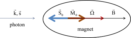
Figure 3: Color online: Geometry of the FMR studied in the paper. Ferromagnet uniformly magnetized by a static magnetic field, ${\bf B}$, is rotating at an angular velocity ${\bf\Omega}$ in the radiation field of circularly polarized photons of wave vector ${\bf k}$ and spin ${\bf s}$. (Due to the negative gyromagnetic ratio, the equilibrium spin of the magnet, ${\bf S}_{0}$, is antiparallel to its equilibrium magnetic moment ${\bf M}_{0}$.)

Within the model of Eq. (38), the rotating magnet placed in the field of a circularly polarized wave feels the oscillating magnetic field that can be represented by a complex function

$$h(t)=h_{0}e^{\pm i\omega^{\prime}t}\,,\quad\omega^{\prime}=\omega\mp\Omega$$ (46)

giving the components of the field as

$$h_{x}={\rm Re}(h),\;h_{y}={\rm Im}(h)\,.$$ (47)

Here $h_{0}$ is the complex amplitude of the wave, $\pm$ sign in Eq. (46) determines the helicity of the wave, while the sign of $\Omega$ determines the direction of rotation of the magnet. Due to the wave the magnetization acquires a small ac-component $m(t)$ (whose real and imaginary parts represent $m_{x}$ and $m_{y}$, respectively),

$$m(t)=\hat{\chi}(\omega)h(t)\,,$$ (48)

where $\hat{\chi}$ is the susceptibility tensor. The absorbed power is given by CT

$$P=\pm i\mu_{0}\omega^{\prime}h_{0}^{*}(\hat{\chi}-{\hat{\chi}}^{\dagger})h_{0}\,.$$ (49)

The problem has, therefore, reduced to the computation of the susceptibility in the rotating frame. The latter can be done by solving the Landau-Lifshitz equation,

$$\frac{d{\bf M}}{dt}=\gamma{\bf M}\times{\bf B}^{(eff)}-\frac{\eta}{M_{0}}|\gamma|{\bf M}\times\left[{\bf M}\times{\bf B}^{(eff)}\right]\,,$$ (50)

in the rotating frame, that is, with ${\bf B}^{(eff)}=-{\delta{\cal{H}}^{\prime}}/{\delta{\bf M}}$ and

$${\cal{H}}^{\prime}=\cal{H}-\frac{\bf M}{\gamma}\cdot{\bf\Omega}-{\bf M}\cdot{\bf h}\,.$$ (51)

The parameter $\eta$ in Eq. (50) is a dimensionless damping coefficient that is responsible for the width of the FMR in the absence of inhomogeneous broadening.

Substituting ${\bf M}=M_{0}{\bf e}_{z}+{\bf m}$ into Eq. (50) and solving for $\hat{\chi}$ one obtains for the power

$$P_{\pm}=\frac{1}{2}\eta|\gamma|M_{0}\mu_{0}^{2}|h_{0}|^{2}f_{\pm}(\omega^{\prime})\,,$$ (52)

where

$$f_{\pm}=\frac{{\omega^{\prime}}^{2}[2({\omega^{\prime}}^{2}-{\omega^{\prime}}_{FMR}^{2})\pm 2{\omega^{\prime}}(\omega^{\prime}_{x}+\omega^{\prime}_{y})+(\omega^{\prime}_{x}+\omega^{\prime}_{y})^{2}]}{({\omega^{\prime}}^{2}-{\omega^{\prime}}_{FMR}^{2})^{2}+\eta^{2}\omega^{\prime 2}(\omega^{\prime}_{x}+\omega^{\prime}_{y})^{2}}\,.$$ (53)

Notice that when there is a full rotational symmetry, $\omega^{\prime}_{x}=\omega^{\prime}_{y}=\omega^{\prime}_{FMR}$, the absorbed power at the resonance is non-zero only for one polarization of the wave that corresponds to the upper sign in Eqs. (46) and (53). This is a consequence of the selection rule due to conservation of the $Z$-component of the total angular momentum (absorbed photon + excited magnet).

Let us now consider a rotating ferromagnet in the radiation field of a linearly polarized electromagnetic wave. In the rotating frame the complex magnetic field of such a wave is

$$h(t)=\frac{h_{0}}{2}\left[e^{i(\omega-\Omega)t}+e^{-i(\omega+\Omega)t}\right]=h_{0}e^{-i\Omega t}\cos(\omega t)$$ (54)

Repeating the above calculation, one obtains for the power averaged over the period of rotation

$$P=\frac{1}{8}\eta|\gamma|M_{0}\mu_{0}^{2}|h_{0}|^{2}\left[f_{+}(\omega-\Omega)+f_{-}(\omega+\Omega)\right]\,.$$ (55)

When the rotational symmetry of the magnet is broken, $\omega_{x}\neq\omega_{y}$, $\kappa>1$, the absorption has two maxima of uneven height at

$$\omega=\omega_{FMR}-(\kappa\mp 1)\Omega\,.$$ (56)

As the rotational symmetry is gradually restored, $\omega_{x}\rightarrow\omega_{y}$, $\kappa\rightarrow 1$, the rotational shift in the position of the main maximum disappears. In that limit the shift in the position of a smaller maximum approaches $2\Omega$ while the height of that maximum goes to zero, see Fig. 4.

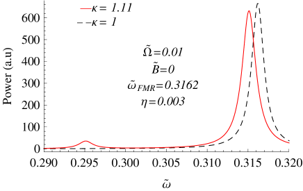
Figure 4: Color online: Absorption of power of linearly polarized electromagnetic radiation by a rotating magnet. Frequencies are given in the units of $\gamma\mu_{0}M_{0}$. As the rotational symmetry is violated the FMR becomes shifted and the second FMR line emerges separated by $2\Omega$ from the first line.

VII Discussion

We have computed the frequency shift of the magnetic resonance due to rotation of the sample. The effect of rotation on the ESR, NMR, and FMR has been studied. We found that it is, generally, quite different from the rotational Doppler effect reported in other systems Padgett2006 . The differences stem from the observation that the spin of an electron or an atom would be insensitive to the rotation of the body as whole if not for the relativistic spin-orbit coupling. Even with account of spin-orbit interactions the spin would not simply follow the rotation of the body but would exhibit more complex behavior described by the dynamics of the angular momentum. Everyone who watched the behavior of a gyroscope in a rotating frame would easily appreciate this fact.

We found the following common features of the magnetic resonance in a rotating sample.

• If the spin Hamiltonian is invariant with respect to the rotation, then the rotation of the body has no effect on the frequency of the resonant absorption of a circularly polarized electromagnetic wave.

• As the rotational invariance is violated, the absorption line shifts. The shift is different from the angular velocity of rotation, $\Omega$. It depends on the degree of violation of the rotational symmetry. The frequency shift goes to zero when the symmetry is restored.

• In the case of a linearly polarized radiation a second resonance line emerges, separated by $2\Omega$ from the first line. The intensity of that line depends on the degree of violation of rotational symmetry. It disappears when the rotational symmetry is restored.

ESR and FMR measurements are usually performed in the GHz range, with the width of the resonance being sometimes as low as a few MHz. Currently available small mechanical rotors can rotate as fast as $100$kHz, which, nevertheless, is still low compared to the linewidths of ESR and FMR. Note, however, that the position of the ESR or FMR maximum can be determined with an accuracy of a few hundred kHz. It is then not out of question that under appropriate conditions the RDE frequency shift and the splitting of the resonance can be observed in high precision ESR and FMR experiments even when the rotation frequency is significantly lower than the linewidth. Since anisotropy of the sample is needed to provide rotational asymmetry, the measurements should be performed on single crystals. Crystals with significant anisotropy of the gyromagnetic tensor should be selected for ESR experiments. When the magnetocrystalline anisotropy is weak, the RDE in FMR can be induced by the asymmetric shape of the sample alone due to the anisotropy of dipole-dipole interactions. Even in this case, however, a single crystal would be preferred to provide a narrow linewidth. Same applies to experiments on RDE in solid state NMR. The NMR frequency range is much lower than that used in ESR and FMR experiments. The width of the NMR line can be as low as a few kHz, that is, well below the available rotational angular velocities. The key to the observation of RDE in a solid state NMR must be the use of a crystal having magnetic order and strong anisotropy of the hyperfine interaction.

A separate interesting question is magnetic resonance in small magnetic particles that are free to rotate. Particles of size in the nanometer range can easily be excited into rotational states with $\Omega$ of hundreds of MHz. Contrary to the rotational quantum states of molecules that have been studied for decades, analytical solution of the problem of a quantum-mechanical rotator does not exist even without a spin. Presence of the spin interacting with a mechanical rotation complicates this problem even further. Rigorous solution has been recently found for the low energy states of a rotator that can be treated as a two-state spin system CG-2010 . General solution is very difficult to obtain. In the case when a particle consists of a large number of atoms, one can develop a semiclassical approximation in which ${\bf\Omega}$ is replaced with ${\bf L}/I$ (with $I$ being the moment of inertia). This suggests that the magnetic resonance in nanoparticles that are free to rotate would split into many lines related to the quantization of ${\bf L}$. Some evidence of this effect has been recently found in the FMR studies of magnetic particles in nanopores FR . Rapid progress in measurements of single magnetic nanoparticles Wern-08 may shed further light on their quantized rotational states and related spin resonances.

VIII Acknowledgements

S.L. acknowledges financial support from Grupo de Investigación de Magnetismo de la Universitat de Barcelona. The work of E.M.C. has been supported by the grant No. DMR-0703639 from the U.S. National Science Foundation and by Catalan ICREA Academia. J.T. acknowledges financial support from ICREA Academia.

References

- (1) H. J. Hay, J. P. Schiffer, T. E. Cranshaw, and P. A. Egelstaff , Phys. Rev. Lett. 4, 165 (1960); D. C. Champeney and P. B. Moon, Proc. Phys. Soc. 77, 350 (1961); W. Kündig, Phys. Rev. 129, 2371 (1963).
- (2) A. L. Kholmetskii, T. Yarman, and O. V. Missevitch, Phys. Scr. 77, 035302 (2008); A. L. Kholmetskii, T. Yarman, O. V. Missevitch, and B. I. Rogozev, Phys. Scr. 79, 065007 (2009).
- (3) B. A. Garetz and S. Arnold, Opt. Commun. 31, 1 (1979).
- (4) R. Simon, H. J. Kimble, and E. C. G. Sundarshan, Phys. Rev. Lett. 61, 19 (1988).
- (5) F. Bretenaker and A. Le Floch, Phys. Rev. Lett. 65, 2316 (1990).
- (6) I.V. Basistiy, A.Y. Bekshaev, M.V. Vasnetsov, V.V. Slyusar, and M. S. Soskin, JETP Lett. 76, 486 (2002).
- (7) L. Chen and W. She, Optics Express 16, 14629 (2008).
- (8) G. Nienhuis, Opt. Commun. 132, 8 (1996).
- (9) J. Courtial, K. Dholakia, D. A. Robertson, L. Allen, and M. J. Padgett, Phys. Rev. Lett. 80, 3217 (1998); J. Courtial, D. A. Robertson, K. Dholakia, L. Allen, and M. J. Padgett, Phys. Rev. Lett. 81, 4828 (1998).
- (10) S. Barreiro, J.W. R. Tabosa, H. Failache, and A. Lezama, Phys. Rev. Lett. 97, 113601 (2006).
- (11) M. Padgett, Nature 443, 924 (2006).
- (12) See, e.g., X. Xu, S. Yin, R. Moro, and W. A. de Heer, Phys. Rev. Lett. 95, 237209 (2005), and references therein.
- (13) J. Tejada, R. D. Zysler, E. Molins, and E. M. Chudnovsky, Phys. Rev. Lett. 104, 027202 (2010).
- (14) R. Tycko, Phys. Rev. Lett. 58, 2281 (1987).
- (15) M. V. Berry, Proc. Roy. Soc. London, Ser. A 392, 45 (1984).
- (16) I. Bialynicki-Birula and Z. Bialynicka-Birula, Phys. Rev. Lett. 78, 2539 (1997).
- (17) N. Ashby, Living Rev. Relativity 6, 1 (2003), and references therein.
- (18) J. D. Anderson and B. Mashhoon, Phys. Lett. A 315, 199 (2003).
- (19) B. Mashhoon, Phys. Rev. A 47 4498 (1993). C. Chicone and B. Mashhoon, Ann. Phys. (Leipzig) 11, 309 (2002); C. Chicone and B. Mashhoon, Phys. Lett. A 298, 229 (2002).
- (20) L. D. Landau and E. M. Lifshitz, The Classical Theory of Fields, Vol. 2 of Course of Theoretical Physics, 4th ed. (Pergamon, New York, 1975).
- (21) L. D. Landau and E. M. Lifshitz, Mechanics, Vol. 1 of Course of Theoretical Physics, 3rd ed. (Pergamon, New York, 1982).
- (22) See, e.g., A. Messiah, Quantum Mechanics, Vol. II (Wiley, New York, 1976).
- (23) F. W. Hehl and W.-T. Ni, Phys. Rev. D 42, 2045 (1990).
- (24) E. M. Chudnovsky, Phys. Rev. Lett. 72, 3433 (1994); E. M. Chudnovsky and X. Martínez Hidalgo, Phys. Rev. B 66, 054412 (2002).
- (25) F. Hartman-Boutron, P. Politi, and J. Villain, Int. J. Mod. Phys. B 10, 2577 (1996).
- (26) E. M. Chudnovsky, D. A. Garanin, and R. Schilling, Phys. Rev. B 72, 094426 (2005).
- (27) E. M. Chudnovsky and J. Tejada, Lectures on Magnetism (Rinton Press, Princeton, NJ, 2008).
- (28) C. Calero, E. M. Chudnovsky, an D. A. Garanin, Phys. Rev. Lett. 95, 166603 (2005).
- (29) C. Kittel. Phys. Rev. 73, 155 (1948).
- (30) E. M. Chudnovsky and D. A. Garanin, Phys. Rev. B 81, 214423 (2010).
- (31) L. Bogani and W. Wernsdorfer, Nature Materials 7, 179 (2008).