Ferrimagnetism of the magnetoelectric compound Cu₂OSeO₃ probed by ⁷⁷Se NMR

Abstract

We present a thorough ⁷⁷Se NMR study of a single crystal of the magnetoelectric compound Cu₂OSeO₃. The temperature dependence of the local electronic moments extracted from the NMR data is fully consistent with a magnetic phase transition from the high-T paramagnetic phase to a low-T ferrimagnetic state with 3/4 of the Cu²⁺ ions aligned parallel and 1/4 aligned antiparallel to the applied field of 14.09 T. The transition to this 3up-1down magnetic state is not accompanied by any splitting of the NMR lines or any abrupt modification in their broadening, hence there is no observable reduction of the crystalline symmetry from its high-T cubic P2₁3 space group. These results are in agreement with high resolution x-ray diffraction and magnetization data on powder samples reported previously by Bos et al. [Phys. Rev. B, 78, 094416 (2008)]. We also develop a mean field theory description of the problem based on a microscopic spin Hamiltonian with one antiferromagnetic ($J_{\text{afm}}\simeq 68$ K) and one ferromagnetic ($J_{\text{fm}}\simeq-50$ K) nearest-neighbor exchange interaction.

I Introduction

Multiferroic and magnetoelectric materials are currently at the center of intense research activity.Eerenstein ; Spaldin ; Khomskii ; Wang In magnetoelectric compounds the application of an electric field can induce a finite magnetization and similarly an electric polarization can be induced by an applied magnetic field.Landau ; Dzyaloshinskii Combining electronic and magnetic properties is an exciting playground for fundamental research which may also lead to new multifunctional materials with potential technological applications. Khomskii ; Gajek ; Wood Since both time-reversal and spatial-inversion symmetries must be broken in ferroic materials,Fiebig magnetoelectric (ME) effects are allowed only in 58 out of the 122 magnetic point groups.Fiebig ; Schmid Along with the weakness of the ME effect, this results in a limited number of compounds displaying ME properties, such as Cr₂O₃Folen , Gd₂CuO₄Wiegelmann , and BaMnF₄Fox . Even though ME materials have been studied extensively in the past decades the recent discovery of the multiferroic compounds TbMnO₃Kimura and TbMn₂O₅Hur , where ferroelectricity (FE) is driven directly by the spin order, has led to a revival of interest in ME systems. The magnetic state in these compounds is either a spiral (as in TbMnO₃,Kimura Ni₃V₂O₈,Lawes0 and MnWO₄Lautenschl ; Taniguchi ), or a collinear configuration (as in Ca₃(CoMn)₂O₆,Choi and FeTe₂O₅BrPregelj ).

Considerable interest has also been drawn to the investigation of ME effects appearing in non-polar systems such as SeCuO₃,Lawes TeCuO₃,Lawes and Cu₂OSeO₃Bos . The latter, as reported recently by Bos et al.,Bos , undergoes a ferrimagnetic phase transition at $T_{c}\simeq 60$ K which is accompanied by a significant magnetocapacitance signal and an anomaly of the dielectric constant. However, high resolution powder x-ray diffraction (XRD) data show that the lattice remains metrically cubic down to 10 K, and this excludes a ME coupling mechanism that involves a spontaneous lattice strain. This result is further supported by recent infrared,Miller and RamanGnezdilov studies. In this respect, Cu₂OSeO₃ appears to be a unique example of a metrically cubic material that allows for piezoelectric as well as linear magnetoelectric and piezomagnetic coupling.

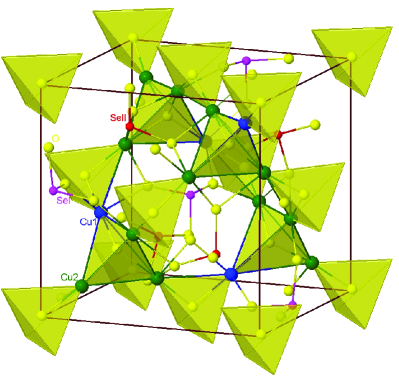
Figure 1: (Color online) Crystal structure of Cu₂OSeO₃. Copper atoms (Cu₁ in blue and Cu₂ in green) form a network of distorted corner sharing tetrahedra. Only the ions inside the unit cell are shown. Oxygen atoms are shown in yellow while Se${}_{\textrm{I}}$ and Se${}_{\textrm{II}}$ ions are shown in magenta and red respectively.

Here we present an extensive ⁷⁷Se Nuclear Magnetic Resonance (NMR) study which highlights the local magnetic and structural properties of Cu₂OSeO₃. Our NMR measurements are performed in a single crystal of Cu₂OSeO₃ as a function of temperature and by varying the direction of the applied magnetic field with respect to the crystalline axes. A detailed analysis of the ⁷⁷Se spectra based on space group symmetry considerations leads to the following main conclusions: The temperature dependence of the local electronic moments extracted from the NMR data is fully consistent with a phase transition between the high-T paramagnetic phase and a low-T ferrimagnetic configuration with 3/4 of the Cu²⁺ moments (type Cu₂) aligned parallel and 1/4 (type Cu₁) aligned antiparallel to the applied field. This 3up-1down state has 1/2 of the saturated magnetization value and is the one proposed by Bos et alBos . The transition is not accompanied by any observable change in the broadening of the NMR lines or any clear splitting, showing that there is no observable symmetry reduction in the crystalline structure from the high-temperature P2₁3 space group, in agreement with the reported powder XRD data.Bos In addition, we provide a microscopic description of the problem based on a spin Hamiltonian with two nearest-neighbor exchange couplings: one antiferromagnetic ($J_{\text{afm}}\simeq 68$ K) between Cu₁ and Cu₂ ions, and one ferromagnetic ($J_{\text{fm}}\simeq-50$ K) between Cu₂ ions. The mean field theory predictions of this model are in good qualitative agreement with the behavior of the local moments extracted from NMR and magnetization data.

The article is organized as follows. In Sec. II we summarize the synthesis process and give some technical details of our experimental procedure. In Sec. III.1 we present our NMR spectra and give a first discussion of some central findings. The theoretical framework for the explanation of the NMR spectra is given in Sec. III.2 based on symmetry considerations. The comparison to the NMR data is then given in Sec. III.3, where we also extract the relevant transferred hyperfine field parameters as well as the T-dependence of the local moments of both types of Cu²⁺ ions. A comparison to the mean field theory predictions is also made here. Our NMR results for the nuclear spin-lattice $1/T_{1}$ and spin-spin $1/T_{2}$ relaxation rates are presented in Sec. IV. We conclude in Sec. V with a brief discussion of our results.

II Synthesis and Experimental details

Single crystals of Cu₂OSeO₃ were grown by the standard chemical vapour phase method. Mixtures of high purity CuO (Alfa-Aesar, 99.995%) and SeO₂ (Alfa-Aesar, 99.999%) powder in molar ratio 2:1 were sealed in quartz tubes with electronic grade HCl as the transport gas for the crystal growth. The ampoules were then placed horizontally into a tubular two-zone furnaces and heated very slowly by 50^∘C/h to 600^∘C. The optimum temperatures at the source and deposition zones for the growth of single crystals have been 610^∘C and 500^∘C, respectively. After six weeks, many dark green, almost black Cu₂OSeO₃ crystals with a maximum size of 8x6x3 mm were obtained.

The orientation of the crystal axes with respect to the crystal faces were determined by Laue X-ray back-scattering measurements and by single crystal X-ray diffraction. The diffraction data are in agreement with previously published data.Effenberger ; Bos ; Larranaga The crystal structure of Cu₂OSeO₃ which belongs to the cubic space group P2₁3 is presented in Fig. 1. The structure is a three-dimensional array of distorted corner-sharing copper tetrahedra. The unit cell consists of 16 Cu²⁺ ions which belong to two crystallographically different groups denoted here by Cu${}_{\text{1}}$ and Cu${}_{\text{2}}$, in 4$\alpha$ and 12b sites respectively. The oxygen atoms form two different types of distorted CuO₅ polyhedra, i.e., trigonal bipyramidal polyhedra for Cu${}_{\text{1}}$ sites and square pyramidal polyhedra for Cu${}_{\text{2}}$ sites. The CuO₅ polyhedra are connected by sharing edges and corners. Similarly, the unit cell contains two crystallographically inequivalent groups of Se⁴⁺ ions, Se${}_{\text{I}}$ and Se${}_{\text{II}}$, each one with multiplicity 4. The two types of SeO₃ (lone pair) trigonal pyramids share corners with the CuO₅ polyhedra.

Figure 2: ⁷⁷Se NMR line shape measurements at 220 K in an external field of 14.09 T applied parallel to the [111], [110] and [100] crystallographic directions.

Table 1: The experimentally observed paramagnetic shifts $\Delta\nu^{exp}$ (in kHz) at $T=220$ K measured with the external magnetic field $\mathbf{H}_{0}$ along the [111], [110] and [100] crystallographic directions.

	$\Delta\nu^{exp}_{[111]}$	$\Delta\nu^{exp}_{[110]}$	$\Delta\nu^{exp}_{[100]}$
$\textrm{P}_{1}$	-121.8$\pm$0.1	-142.9 $\pm$0.1	-96.6 $\pm$0.01
$\textrm{P}_{2}$	-49.4$\pm$0.2	-53.9 $\pm$0.1	137.5 $\pm$0.04
$\textrm{P}_{3}$	89.9$\pm$0.1	60.9 $\pm$0.1
$\textrm{P}_{4}$	277.1$\pm$0.2	206.8 $\pm$0.1

Pulsed NMR experiments were carried out on ⁷⁷Se nuclei with nuclear spin $I=1/2$, gyromagnetic ratio $\gamma_{N}/2\pi=8.1179$ MHz/T and natural abundance 7.58$\%$. The NMR experiments were performed on a 125 mg single crystal at an Oxford 14.09 T magnet equipped with a variable temperature insert utilizing a home built spectrometer. The echo signal was produced by a standard Hahn echo pulse sequence with a typical $\pi/2$ pulse length of 6 $\mu s$. The separation between the two echo-generating pulses was 20$-$60 $\mu s$ depending on the experimental conditions. The ⁷⁷Se NMR spectra were measured by Fourier transform (FT) of the half spin-echo signal whenever the whole line could be irradiated with one radiofrequency pulse. For the broad lines, the spectrum was obtained by plotting the area of the echo as a function of the irradiation frequency (frequency sweep). The nuclear spin-lattice $T_{1}$ and spin-spin $T_{2}$ relaxation times were measured using the standard spin echo pulse sequence combined with the saturation recovery method for $T_{1}$ measurements. For the analysis of the NMR data we have measured the magnetization of a 28.86 mg single crystal of Cu₂OSeO₃ at 14 T using a Quantum Design PPMS (Physical Properties Measurement System) apparatus located in the Trinity College in Dublin, Ireland.

III ⁷⁷Se Nuclear Magnetic Resonance spectra

III.1 General results

The nuclear ⁷⁷Se spins provide a powerful local probe of the behavior of the electronic Cu²⁺ moments through the transferred hyperfine and the magnetic dipolar mechanisms. Here we have performed detailed ⁷⁷Se NMR lineshape measurements at 14.09 T with the magnetic field applied parallel to the crystallographic directions [111], [110] and [100]. Figure 2 shows the ⁷⁷Se NMR spectrum at $T=220$ K. There appear four distinct resonance lines when the field is applied along [111] and [110], while two lines are observed along the [100] direction. The specific values of the shifts of the lines $\Delta\nu=\nu-\nu_{L}$ from the bare Larmor frequency $\nu_{L}$ are provided in Table 1. The integrated areas under these lines are found with the relative ratios 3:1:3:1 for [111], 2:2:2:2 for [110], and 4:4 for [100]. Since the area under a given line is proportional to the number of the nuclei that resonate in the corresponding frequency window, we conclude that there are four magnetically inequivalent groups of ⁷⁷Se sites in the [111] and [110] directions and only two groups for [100]. It is clear that the latter correspond to the two crystallographically inequivalent groups of selenium sites Se${}_{\textrm{I}}$ and Se${}_{\textrm{II}}$ which have the same multiplicity (four per unit cell). On the other hand, both Se${}_{\textrm{I}}$ and Se${}_{\textrm{II}}$ groups split into two magnetically inequivalent subgroups when the field is along [111] and [110] with multiplicities 3:1 and 2:2 respectively. Below in Sec. III.2, we shall be able to identify these specific subgroups of Se sites (and even retrieve the values of the corresponding elements of the transferred hyperfine tensor) by taking into account the local symmetry around each Se site under the conditions that (1) we are in the 3up-1down state and (2) that the crystalline structure belongs to P2₁3 space group. The second condition is an important issue since any symmetry reduction of the crystal from P2₁3 to either of the two possible crystallographic subgroups R3 or P2₁2₁2₁,IntTablesCryst will result in partially or fully splitting of the above multiple lines.

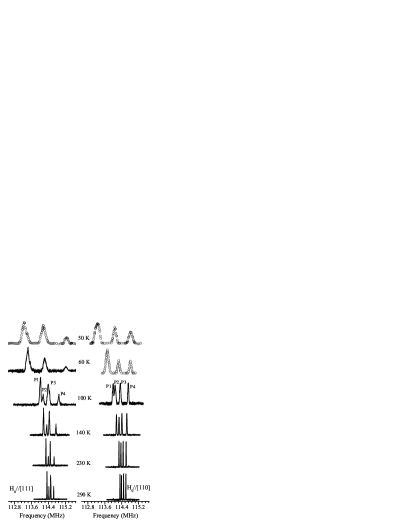
Figure 3: ⁷⁷Se NMR line shape measurements for selected temperatures measured at external field of 14.09 T applied parallel to the [111] and [110] crystallographic directions.

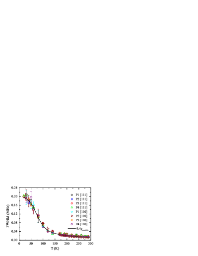
Figure 4: (Color online) Temperature dependence of the ⁷⁷Se NMR full width at half maximum (FWHM) for each of the four spectral lines measured at 14.09 T along the [111] and [110] crystallographic directions. The FWHM for lines P1 and P3 along [111] are multiplied by a factor 0.9 and 0.7 respectively in order to match the other curves. The temperature dependence of the magnetic susceptibility per copper mol (multiplied by a factor of 9.4) as measured with the magnetometer at 14 T is shown with a solid line.

Let us now examine what happens as we cool down the system. We have studied the temperature dependence of the NMR spectra in the range 20-290 K with the magnetic field applied along [111] and [110]. Some representative NMR spectra are shown in Fig. 3. We first note that the lines P1 and P2 get gradually closer to each other below 100 K and merge into a single peak at lower temperatures. We also find a gradual increase in the line broadenings or Full Width at Half Maximum (FWHM). However, as we show in Fig. 4, all the NMR line broadenings (shown with symbols in Fig. 4) follow quite closely the corresponding gradual increase of the magnetization as measured by PPMS (solid line). This being the typical behavior of inhomogeneous broadening, together with the fact that we find no observable splitting of any of the multiple lines, we are lead to conclude that there is no clear sign of any symmetry reduction of the crystalline structure as the system enters the ferrimagnetic state.

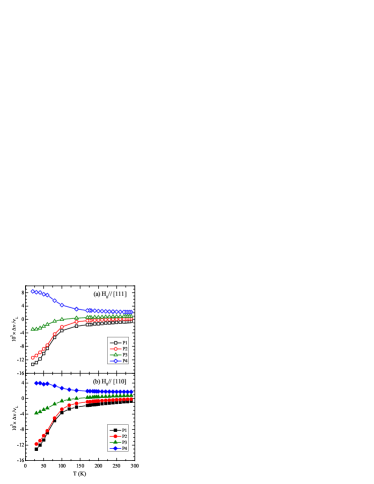
Figure 5: (Color online) Temperature dependence of the relative NMR shifts $\Delta\nu/\nu_{L}$ at H${}_{0}=14.09$ T and for each of the four spectral lines observed along the (a) [111] and (b) [110] crystallographic directions.

Another important issue is the behavior of the line shifts as we cool down the system, since this is governed by the corresponding ordering behavior of the electronic Cu²⁺ moments. Figure 5 shows the T-dependence of the relative shifts $\Delta\nu/\nu_{L}$ measured at H${}_{0}=14.09$ T for fields applied along the directions [111] and [110]. From these data, as we show below in Sec. III.2, we shall be able to extract the T-dependence of the local moments of both Cu${}_{\text{1}}$ and Cu${}_{\text{2}}$ ions and thus confirm the ferrimagnetic nature of the low-T phase of this compound.

III.2 Theoretical analysis

In order to understand and analyze the above NMR data we first note that the most relevant terms in the nuclear spin-1/2 Hamiltonian for the $k$-th Se site are (i) the Zeeman coupling with the external field $\mathbf{H}_{0}$, (ii) the transferred-hyperfine interactions with the relevant neighboring Cu spins and (iii) the dipolar interactions with all the electronic Cu spins, namely

$$\mathcal{H}_{k}=-\gamma_{N}\hbar\mathbf{I}_{k}\cdot\left(\left(1+\mathbf{K}^{c}_{k}\right)\cdot\mathbf{H}_{0}+\mathbf{H}_{k}^{\textrm{tr}}+\mathbf{H}_{k}^{\textrm{dip}}\right)~{},$$ (1)

where $\mathbf{K}^{c}_{k}$ denotes the chemical shift tensor, while $\mathbf{H}_{k}^{\textrm{tr}}$ and $\mathbf{H}_{k}^{\textrm{dip}}$ are the local effective fields resulting from the transferred-hyperfine and the dipolar interactions respectively.

Transferred-hyperfine contribution.— Let us discuss the transferred-hyperfine coupling first. The transferred-hyperfine interaction is local, i.e. it involves a ⁷⁷Se nuclear spin and its six nearest neighbor Cu ions, and is mediated through the Cu-O-Se bonding. The local transferred-hyperfine field experienced by the $k$-th nuclear spin can be written as

$$\mathbf{H}^{\textrm{tr}}_{k}=q\sum_{j}\mathbf{A}_{k}^{j}\cdot\mathbf{M}_{j}~{},$$ (2)

where $q\equiv 1/(\gamma_{N}\hbar g\mu_{B})$, $\mathbf{M}_{j}=-g\mu_{B}\langle\mathbf{S}_{j}\rangle$ denote the local moments of the six neighbor Cu ions, $\mu_{B}$ is Bohr’s magneton, and $g$ is the spectroscopic factor with $g\simeq 2.11$.Larranaga To go beyond this general description we need to exploit the local symmetry properties of the electronic environment of each Se site. As we mentioned in the introduction, each unit cell contains four crystallographically equivalent sites of Se${}_{\textrm{I}}$ ions and similarly four equivalent sites of Se${}_{\textrm{II}}$ ions. We denote these by Se${}_{\textrm{I}}^{n}$ and Se${}_{\textrm{II}}^{n}$ respectively, where $n=1,\ldots,4$. We start our analysis with the first type of selenium ions. As can be seen in Fig. 6, each Se${}_{\textrm{I}}^{n}$ ion sits on a high symmetry crystal site. Each oxygen of the trigonal pyramid SeO₃ is connected to two different types of copper ions, denoted as Cu₁ and Cu₂. The three Se${}_{\textrm{I}}$-O-Cu₁-Cu₂ bonding groups are equivalent and are mapped to one another by a rotation of $120^{\circ}$ around a 3-fold symmetry axis. This $\mathcal{C}_{3}$ axis passes through the selenium site and is vertical to the plane of the three Cu₂ ions. This plane is parallel and slightly above the plane formed by the three Cu₁ ions, as well as to the plane formed by the three oxygen atoms (see Fig. 6). Thus the transferred hyperfine interaction at any given Se${}_{\textrm{I}}^{n}$ site can be described by two hyperfine tensors, $\mathbf{A}^{\textrm{Cu}_{1}}_{\textrm{Se}^{n}_{\textrm{I}}}$ and $\mathbf{A}^{\textrm{Cu}_{2}}_{\textrm{Se}^{n}_{\textrm{I}}}$. The former (latter) represents the sum of the three hyperfine tensors between the $n$-th Se${}_{\textrm{I}}$ and the three Cu₁ (Cu₂) ions. Now, one of the two 3-fold rotations reads $(x,y,z)\mapsto(z,x,y)$, and this transforms the elements of any second rank tensor as

$$\begin{pmatrix}xx&xy&xz\\ yx&yy&yz\\ zx&zy&zz\\ \end{pmatrix}\mapsto\begin{pmatrix}zz&zx&zy\\ xz&xx&xy\\ yz&yx&yy\\ \end{pmatrix}.$$ (3)

Since this is a symmetry operation we must have $xx=yy=zz$ and $xy=xz=yz$. These conditions describe an axially symmetric tensor with the third principal eigenvector along the [111] direction. Thus the hyperfine tensors $\mathbf{A}^{\textrm{C}u_{1}}_{\textrm{S}e^{n}_{1}}$ and $\mathbf{A}^{\textrm{C}u_{2}}_{\textrm{S}e^{n}_{\textrm{I}}}$ are also axially symmetric and their principal axes system can be assigned easily. One is the 3-fold axis ($\mathbf{e}_{3}$) while for the remaining two we may take any pair of mutually perpendicular axes (denoted by $\mathbf{e}_{1}$ and $\mathbf{e}_{2}$) on the plane formed by the three Cu₂ (or Cu₁) neighboring ions. Thus we may write

$$q\mathbf{A^{\textrm{C}u_{1}}_{\textrm{S}e^{n}_{\textrm{I}}}}=\begin{pmatrix}\alpha_{\textrm{tr}}&0&0\\ 0&\alpha_{\textrm{tr}}&0\\ 0&0&\beta_{\textrm{tr}}\\ \end{pmatrix},q\mathbf{A^{\textrm{C}u_{2}}_{\textrm{S}e^{n}_{\textrm{I}}}}=\begin{pmatrix}\alpha^{\prime}_{\textrm{tr}}&0&0\\ 0&\alpha^{\prime}_{\textrm{tr}}&0\\ 0&0&\beta^{\prime}_{\textrm{tr}}\\ \end{pmatrix}~{},$$ (4)

where we emphasize that each tensor is written in its own principal axes frame. In what follows the above diagonal elements are treated as fitting parameters.

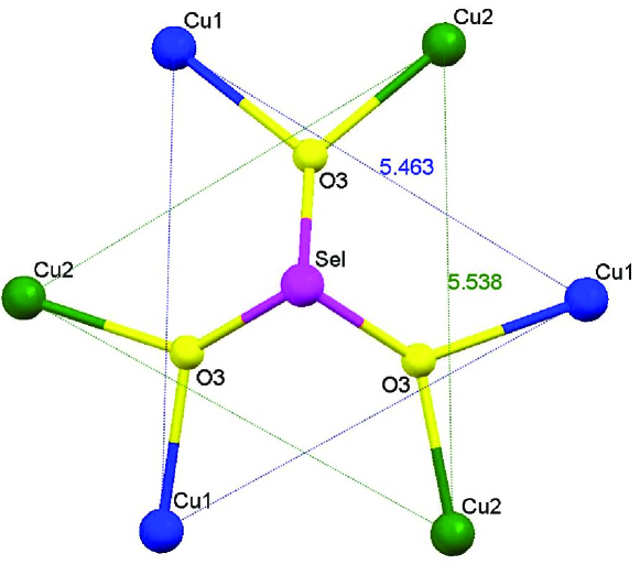
Figure 6: (Color online) The local environment of each Se${}_{\textrm{I}}$ nuclear site. There is a 3-fold symmetry axis through the Se site which is vertical to the planes of the Cu${}_{\text{1}}$ and Cu${}_{\text{2}}$ ions. Note that the plane of the Cu${}_{\text{2}}$ ions lies slightly above the plane of the Cu${}_{\text{1}}$ ions. Shown distances are in units of $\AA$.

We now turn to the local symmetry of the Se${}_{\textrm{II}}^{n}$ ions. These are bonded through oxygen sites to six Cu₂ ions (Fig. 7) which belong to two parallel planes. As in the case of the Se${}_{\textrm{I}}^{n}$ sites, a 3-fold rotation axis is again present and this passes through the selenium site of the trigonal pyramid SeO₃ and is vertical to the set of planes defined by the Cu₂ ions. The hyperfine interactions at each Se${}_{2}^{n}$ site can thus be described with one hyperfine tensor, $\mathbf{A}^{\textrm{C}u_{2}}_{\textrm{S}e^{n}_{\textrm{II}}}$, which stands for the sum of the hyperfine tensors of all six neighboring Cu₂ ions. Due to the 3-fold axis this tensor is axially symmetric and, as explained for the Se${}_{\textrm{I}}$ case, the principal axes are the 3-fold axis and the two mutually perpendicular axes (their plane is parallel to the two Cu planes). Written in its own principal axis system, the hyperfine tensor $\mathbf{A}^{\textrm{C}u_{2}}_{\textrm{S}e^{n}_{\textrm{II}}}$ can thus be written as

$$q\mathbf{A^{\textrm{C}u_{2}}_{\textrm{Se}_{\textrm{II}}^{n}}}=\begin{pmatrix}\delta^{\prime}_{\textrm{tr}}&0&0\\ 0&\delta^{\prime}_{\textrm{tr}}&0\\ 0&0&\vartheta^{\prime}_{\textrm{tr}}\\ \end{pmatrix}~{}.$$ (5)

Summarizing, the hyperfine tensors for each one of the four Se${}^{n}_{\textrm{I}}$ sites (respectively Se${}^{n}_{\textrm{II}}$ sites) of the unit cell have the form of Eqs. 4 (resp. 5) as long as they are written in their own local principal axis coordinate frame. In Table 2 we provide the coordinates of the unit vector $\mathbf{e}_{3}$ in the (x,y,z) frame for each of the eight selenium sites in the unit cell. The coordinate frames of the hyperfine tensors for the four Se${}^{n}_{\textrm{I}}$ and the four Se${}^{n}_{\textrm{II}}$ sites are related with proper rotation of their principal axes $[\mathbf{e}_{1},\mathbf{e}_{2},\mathbf{e}_{3}]$.

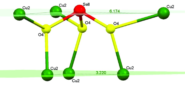
Figure 7: (Color online) The local environment of Se${}_{\textrm{II}}$ type ions. As in the case of Se${}_{\text{I}}$ ions, there is a 3-fold symmetry axis through the Se site which is vertical to the planes of Cu${}_{\text{2}}$ ions. Shown distances are in units of $\AA$.

Dipolar contribution.— In order to provide a more accurate quantitative description of the measured NMR spectra we must also consider the dipolar coupling. In contrast to the transferred-hyperfine interactions, the dipolar coupling is long-ranged and since we are dealing with a ferrimagnet we must also consider the effect of the demagnetization field. To this end we follow the Lorentz methodWhite which consists of splitting the summation over the dipolar contributions into two parts. In the first we perform a discrete summation over all individual dipolar contributions from all Cu ions enclosed in a sphere of radius $R$ much larger than the lattice spacing and much smaller than the size of the sample. The summation outside this Lorentz sphere gives rise to the demagnetization field $\mathbf{H}^{\text{dem}}$ which can be evaluated using a continuous integration. This gives the well known expressionWhite $\mathbf{H}^{\text{dem}}=4\pi(\frac{1}{3}-\mathbf{N}_{d})\cdot\widetilde{\mathbf{M}}$, where the demagnetizing tensor $\mathbf{N}_{d}$ is specific to the shape of the sample and $\widetilde{\mathbf{M}}=\left(4\mathbf{M}_{1}+12\mathbf{M}_{2}\right)/a^{3}=4\mathbf{M}/a^{3}$ is the total moment divided by the volume of the sample. The demagnetizing tensor is not known but we shall be able to adjust it so that we obtain a reasonable T-dependence of the extracted moments at high temperatures (cf. below).

Following the above, the total dipolar field at the $k$-th Se nuclear site can be written as

$$\mathbf{H}^{\textrm{dip}}_{k}=q\sum_{r_{jk}\leq R}\mathbf{D}_{k}^{j}\cdot\mathbf{M}_{j}+\mathbf{H}^{\text{dem}}~{},$$ (6)

where as usually the cartesian components ($\alpha,\beta=x,y,z$) of the dipolar tensors are given by

$$q\left(\mathbf{D}^{j}_{k}\right)_{\alpha\beta}=-\frac{\delta^{\alpha\beta}}{r_{jk}^{3}}+3\frac{\mathbf{r}_{jk}^{\alpha}\mathbf{r}_{jk}^{\beta}}{r_{jk}^{5}}~{},$$ (7)

where $\mathbf{r}_{jk}$ stands for the displacement vector from the $k$-th nuclear site to the $j$-th electronic spin. Summing over the two different types of Cu²⁺ ions in Eq. (6) separately we get

$$\mathbf{H}^{\textrm{dip}}_{k}=q\left(\mathbf{D}_{k}^{\textrm{Cu}_{1}}\cdot\mathbf{M}_{1}+\mathbf{D}_{k}^{\textrm{Cu}_{2}}\cdot\mathbf{M}_{2}\right)+\mathbf{H}^{\text{dem}}~{}.$$ (8)

Using the known valuesEffenberger ; Bos ; Larranaga of the positions of the Cu²⁺ moments one may evaluate the summations over the Lorentz sphere with very good accuracy (we find that the sums converge already for $R\sim 5a$). Now, the symmetry of the crystal necessitates that the resulting dipolar tensors have the same principal axes as the corresponding transferred-hyperfine tensors. Indeed written in the corresponding local coordinate frame we find

$$q\mathbf{D^{\textrm{C}u_{1}}_{\textrm{Se}_{\textrm{I}}^{n}}} = \begin{pmatrix}\alpha_{\textrm{dip}}&0&0\\ 0&\alpha_{\textrm{dip}}&0\\ 0&0&\beta_{\textrm{dip}}\\ \end{pmatrix},q\mathbf{D^{\textrm{C}u_{2}}_{\textrm{Se}_{\textrm{I}}^{n}}}=\begin{pmatrix}\alpha^{\prime}_{\textrm{dip}}&0&0\\ 0&\alpha^{\prime}_{\textrm{dip}}&0\\ 0&0&\beta^{\prime}_{\textrm{dip}}\\ \end{pmatrix},$$

$$q\mathbf{D^{\textrm{C}u_{1}}_{\textrm{Se}_{\textrm{II}}^{n}}} = \begin{pmatrix}\delta_{\textrm{dip}}&0&0\\ 0&\delta_{\textrm{dip}}&0\\ 0&0&\vartheta_{\textrm{dip}}\\ \end{pmatrix},q\mathbf{D^{\textrm{C}u_{2}}_{\textrm{Se}_{\textrm{II}}^{n}}}=\begin{pmatrix}\delta^{\prime}_{\textrm{dip}}&0&0\\ 0&\delta^{\prime}_{\textrm{dip}}&0\\ 0&0&\vartheta^{\prime}_{\textrm{dip}}\\ \end{pmatrix}~{},$$ (9)

where, in units of $10^{22}\textrm{cm}^{-3}$: $\alpha_{\textrm{dip}}=1.68$, $\beta_{\textrm{dip}}=-3.37$, $\alpha^{\prime}_{\textrm{dip}}=1.18$, $\beta^{\prime}_{\textrm{dip}}=-2.36$, $\delta_{\textrm{dip}}=-0.58$, $\vartheta_{\textrm{dip}}=1.17$, $\delta^{\prime}_{\textrm{dip}}=-1.3$, and $\vartheta^{\prime}_{\textrm{dip}}=2.61$.

Table 2: The second column gives the unit vector $\mathbf{e}_{3}$ in the fixed (x,y,z) frame for each of the eight Se sites per unit cell (first column). The following columns give the theory predictions for the sum of the dipolar (excluding the demagnetization field) and the transferred hyperfine contributions to the relative NMR shifts, when the field is along the [111], [110], and [100] crystallographic directions. The dimensionless parameters $\widetilde{\alpha},\widetilde{\beta},\widetilde{\delta},\widetilde{\vartheta}$ are defined in Eqs. (10)-(13).

Se	$\mathbf{e}_{3}$	[111]	[110]	[100]
Se${}^{1}_{\textrm{I}}$	(1,1,1)/$\sqrt{3}$	$\widetilde{\beta}$	$(\widetilde{\alpha}+2\widetilde{\beta})/3$	$(2\widetilde{\alpha}+\widetilde{\beta})/3$
Se${}^{2}_{\textrm{I}}$	(1,1,-1)/$\sqrt{3}$	$(8\widetilde{\alpha}+\widetilde{\beta})/9$	$(\widetilde{\alpha}+2\widetilde{\beta})/3$	$(2\widetilde{\alpha}+\widetilde{\beta})/3$
Se${}^{3}_{\textrm{I}}$	(-1,1,1)/$\sqrt{3}$	$(8\widetilde{\alpha}+\widetilde{\beta})/9$	$\widetilde{\alpha}$	$(2\widetilde{\alpha}+\widetilde{\beta})/3$
Se${}^{4}_{\textrm{I}}$	(1,-1,1)/$\sqrt{3}$	$(8\widetilde{\alpha}+\widetilde{\beta})/9$	$\widetilde{\alpha}$	$(2\widetilde{\alpha}+\widetilde{\beta})/3$
Se${}^{1}_{\textrm{II}}$	(1,1,1)/$\sqrt{3}$	$\widetilde{\vartheta}$	$(\widetilde{\delta}+2\widetilde{\vartheta})/3$	$(2\widetilde{\delta}+\widetilde{\vartheta})/3$
Se${}^{2}_{\textrm{II}}$	(1,1,-1)/$\sqrt{3}$	$(8\widetilde{\delta}+\widetilde{\vartheta})/9$	$(\widetilde{\delta}+2\widetilde{\vartheta})/3$	$(2\widetilde{\delta}+\widetilde{\vartheta})/3$
Se${}^{3}_{\textrm{II}}$	(-1,1,1)/$\sqrt{3}$	$(8\widetilde{\delta}+\widetilde{\vartheta})/9$	$\widetilde{\delta}$	$(2\widetilde{\delta}+\widetilde{\vartheta})/3$
Se${}^{4}_{\textrm{II}}$	(1,-1,1)/$\sqrt{3}$	$(8\widetilde{\delta}+\widetilde{\vartheta})/9$	$\widetilde{\delta}$	$(2\widetilde{\delta}+\widetilde{\vartheta})/3$

Predictions for the relative shifts.— Including both the transferred-hyperfine and the dipolar contributions it is straightforward to deduce the relative shifts for each Se site and for each direction of the applied field considered in our experiments. The resulting expressions – without the contribution for the demagnetization field and the chemical shift – are provided in Table 2 in terms of the dimensionless parameters

$$\widetilde{\alpha} = (\alpha_{\textrm{tr}}+\alpha_{\textrm{dip}})\chi_{1}+(\alpha^{\prime}_{\textrm{tr}}+\alpha^{\prime}_{\textrm{dip}})\chi_{2}$$ (10)

$$\widetilde{\beta} = (\beta_{\textrm{tr}}+\beta_{\textrm{dip}})\chi_{1}+(\beta^{\prime}_{\textrm{tr}}+\beta^{\prime}_{\textrm{dip}})\chi_{2}$$ (11)

$$\widetilde{\delta} = \delta_{\textrm{dip}}\chi_{1}+(\delta^{\prime}_{\textrm{tr}}+\delta^{\prime}_{\textrm{dip}})\chi_{2}$$ (12)

$$\widetilde{\vartheta} = \vartheta_{\textrm{dip}}\chi_{1}+(\vartheta^{\prime}_{\textrm{tr}}+\vartheta^{\prime}_{\textrm{dip}})\chi_{2}~{},$$ (13)

where $\chi_{1}=\text{M}_{1}/\text{H}_{0}$ and $\chi_{2}=\text{M}_{2}/\text{H}_{0}$ denote the local susceptibilities per Cu₁ and Cu₂ respectively.

III.3 Comparison with experiment

Let us now compare the theoretical predictions given in Table 2 to our experimental data. We find exact agreement for the number of distinct lines as well as for their relative intensities. When the magnetic field is applied along [111] our model predicts that the group of Se${}_{\text{I}}$ sites give one spectral line for Se${}_{\textrm{I}}^{1}$ and a separate, three times more intense line from Se${}_{\textrm{I}}^{2}$, Se${}_{\textrm{I}}^{3}$ and Se${}_{\textrm{I}}^{4}$. A similar result holds for the group of Se nuclear spins of the second type. In the [110] direction we expect four resonance lines with relative ratio 2:2:2:2, while in the [100] direction we expect two lines with relative ratio 4:4 (see Table 2). These predictions are in perfect agreement with our experimental results shown in Figs. 2 and 3.

For consistency reasons we would like next to contrast the T-dependence of $\widetilde{\alpha}$, $\widetilde{\beta}$, $\widetilde{\delta}$, and $\widetilde{\vartheta}$ obtained from the NMR data along the [111] direction with that obtained from the NMR data along the [110] direction. The results (taken after correcting the data for the chemical shift and the demagnetization field, cf. below) are shown in Fig. 8 and are almost identical. This provides a much stronger confirmation of the internal consistency of the above theory. In addition, Fig. 8 tells us that we may use either the [111] or the [110] data in order to extract, in conjunction with Eqs. (10)-(13), the transferred hyperfine field parameters as well as the T-dependence of the local moments M₁ and M₂. In what follows we have taken the data along [111].

Table 3: Extracted estimates of the components of the transferred hyperfine tensors $\mathbf{A}^{\textrm{Cu}_{1}}_{\textrm{Se}^{n}_{\textrm{I}}}$, $\mathbf{A}^{\textrm{Cu}_{2}}_{\textrm{Se}^{n}_{\textrm{I}}}$ and $\mathbf{A}^{\textrm{C}u_{2}}_{\textrm{S}e^{n}_{\textrm{II}}}$ defined in Eqs. (4) and (5) (here in units of $10^{22}\textrm{cm}^{-3}$) for two possible values of the constant $r_{1}$ defined in the text.

$r_{1}$	$\alpha_{\textrm{tr}}$	$\beta_{\textrm{tr}}$	$\alpha^{\prime}_{\textrm{tr}}$	$\beta^{\prime}_{\textrm{tr}}$	$\delta^{\prime}_{\textrm{tr}}$	$\theta^{\prime}_{\textrm{tr}}$
$-2$	$-2.3$	$12.6$	$-5.0$	$26.8$	$-14.6$	$-14.0$
$-1.2$	$-1.7$	$-5.4$	$-1.2$	$-3.8$	$-16.8$	$-16.2$

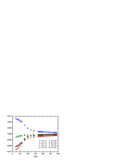
Figure 8: (Color online) A comparison of the values of the parameters given in Eqs. (10)-(13) extracted from the NMR line shifts along the [111] direction with those extracted from the [110] direction.

Assignment of the NMR lines.— The next step is to identify the specific subgroup of Se sites associated to each given NMR line. To this end, we first note that the local fields of Se${}^{n}_{\textrm{I}}$ and Se${}^{n}_{\textrm{II}}$ given in Table 2 map to one another when interchanging $(\widetilde{\alpha},\widetilde{\beta})\mapsto(\widetilde{\delta},\widetilde{\vartheta})$. This prevents a straightforward assignment of the NMR lines to specific subgroup of selenium sites. For example, we cannot infer if it is P1 and P2 or rather P1 and P4 (cf. Fig. 3) that come from the same type of Se sites. We overcome this drawback by comparing the fits in different directions of the applied field. Indeed, by fitting the experimental data of $\Delta\nu^{exp}_{[111]}$ (see Table 1) with the theoretical expressions given in Table 2 we can reproduce the experimental data of both $\Delta\nu^{exp}_{[110]}$ and $\Delta\nu^{exp}_{[100]}$ only under the condition that P1 and P2 come from one group of selenium sites while P3 and P4 come from the other. This result is further supported by the nuclear spin-lattice and spin-spin relaxation time measurements presented in the following section. However it is still not possible at this point to tell whether the pair P1-P2 comes from type-I or type-II Se sites. We have extracted the temperature dependence of the local moments using both possibilities and we have found that the choice which gives the most physically reasonable behavior is the one which assigns the pair P1-P2 to type-II Se sites.

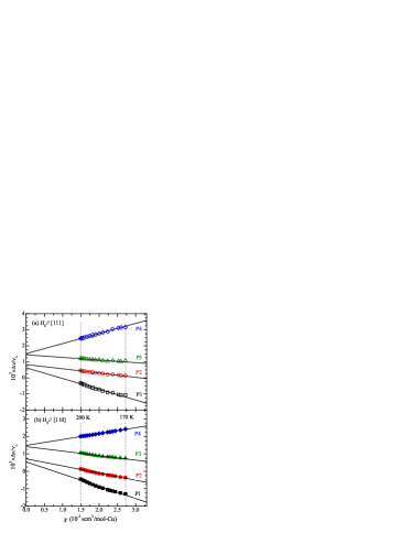
Figure 9: (Color online) The fractional shift $\Delta\nu_{\textrm{P}_{i}}/\nu_{\textrm{L}}$ for each one of the four NMR peaks as measured along (a) [111] and (b) [110], vs. the susceptibility $\chi$ measured with the magnetometer with $T$ being an implicit parameter. The dotted lines indicates the points where $T=170$ K, and $290$ K.

Hyperfine parameters and local susceptibilities.— We are now ready to extract the local moments from the NMR data. We first write the measured susceptibility per Cu and the measured relative shifts $K\equiv\Delta\nu/\nu_{L}$ as

$$\chi_{\textrm{tot}}(T) = \chi_{\text{spin}}(T)+\chi_{\text{dia}}+\chi_{\text{vv}}$$ (14)

$$K(T) = K_{\text{spin}}(T)+K^{c}~{}.$$ (15)

Here $\chi_{\textrm{spin}}=(\chi_{1}+3\chi_{2})/4$ is the total spin susceptibility per Cu, and $\chi_{\text{dia}}$, $\chi_{\text{vv}}$ are the T-independent diamagnetic and van Vleck contributions respectively. Similarly, $K_{\text{spin}}(T)$ includes the dipolar and the transferred hyperfine contributions which were given above in Table 2, while $K^{c}$ stands for the T-independent chemical shift.

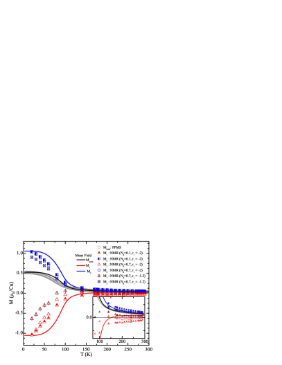
Figure 10: (Color online) Comparison between the total magnetization measured by PPMS (corrected for the van Vleck and diamagnetic contributions) and the local moments extracted from NMR (with two different values of the ratio $r_{1}$, cf. text) with the corresponding mean field theory predictions. We also demonstrate how the value of the demagnetizing factor $N_{d}$ affects the sign of M₁ at high temperatures.

Figure 9(a) shows the so-called Clogston-Jaccarino plotCJ of the four measured shifts $K$ in both [111] and [110] directions versus the measured susceptibility per mol Cu in the high temperature regime. The linear behavior shows that both $\chi_{1}$ and $\chi_{2}$ are proportional to $\chi_{\text{spin}}$ in this regime. We can exploit this linear behavior in order to extract the values of $K^{c}$ for each line if we make an estimate of $\chi_{\text{dia}}+\chi_{\text{vv}}$. For the latter we take the upper bound of $\chi_{\text{dia}}+\chi_{\text{vv}}\simeq 1\times 10^{-4}$ cm³/mol-Cu which is obtained from the comparison of the measured magnetization with the mean field theory prediction (cf. below). We extract the following estimates respectively for the lines P1, P2, P3 and P4: $K^{c}\simeq 5.60\times 10^{-4}$, $8.06\times 10^{-4}$, $14.2\times 10^{-4}$, $15.7\times 10^{-4}$ along [111], while $K^{c}\simeq 4.68\times 10^{-4}$, $6.73\times 10^{-4}$, $13.8\times 10^{-4}$, $15.1\times 10^{-4}$ along [110].

After subtracting the above values of $\chi_{\text{dia}}+\chi_{\text{vv}}$ and $K_{\text{chem}}$ from the bare data, we adopt the following procedure. We first extract an estimate for $\theta_{\text{tr}}^{\prime}$ by using the data for $\widetilde{\theta}$ at the lowest available temperature ($T=20$ K) and the relation M${}_{1}(20K)=r_{1}\text{M}(20K)$, where $r_{1}$ is a constant which measures the effect of quantum fluctuations at low temperatures. Using Eq. (13), the relation M$=$(M${}_{1}+3$M${}_{2})/4$, and the PPMS data for M, we may extract the whole temperature dependence of M₁ and M₂. In turn, Eqs. (10)-(12) can provide the remaining transferred hyperfine parameters in a straightforward way. For comparison, we have used two values of $r_{1}$: The first, $r_{1}=-2$, corresponds to the case without quantum fluctuation effects, while the second value, $r_{1}=-1.2$, corresponds to the reduction in the spin length found by Neutron diffraction data.Bos As for the demagnetization factor, it turns out that for $N_{d}\lesssim 0.6$ the extracted M${}_{1}(T)$ is not positive at room temperatures but saturates to a negative value. However such a behavior would be quite unphysical: Although there is a large antiferromagnetic exchange field on each Cu₁ site since it has 6 neighboring Cu₂ sites, one still expects that M₁ should ultimately change sign at some temperature $T^{*}$ which is above $T_{c}$ but certainly well below room temperature. On this issue, the mean-field theory described below predicts that $T^{*}\simeq 152$ K. So we adjust $N_{d}\simeq 0.7$, which in conjunction with the value of $r_{1}$ can provide a physically more reasonable behavior at high temperatures.

The resulting estimates of the hyperfine parameters are provided in Table 3, while the extracted T-dependence of the local moments is shown in Fig. 10. The major result contained in Fig. 10 is that the NMR data are fully consistent with the 3up-1down ferrimagnetic state, namely that the Cu₂ moments are aligned parallel and the Cu₁ moments are aligned antiparallel to the applied field. Hence NMR on single crystals provides a more direct local probe of this state, mapping out the whole T-dependence of the local moments.

Comparison to microscopic model:— It is worthwhile to contrast the above NMR findings with a microscopic spin model for Cu₂OSeO₃. Following the Kanamori-Goodenough rules (see also discussion in Ref. Bos, ) we introduce two exchange parameters: one ferromagnetic ($J_{\text{fm}}$) between Cu₂-Cu₂ ions and one antiferromagnetic ($J_{\text{afm}}$) between Cu₁-Cu₂ ions. Looking at the structure one finds that each Cu₁ neighbors six Cu₂ ions while each Cu₂ neighbors four Cu₂ ions and two Cu₁ ions. The self-consistent equations of the corresponding mean field theory are given by

$$m_{1} = \text{tanh}\left(\frac{b-3J_{\text{afm}}m_{2}}{2T}\right)$$ (16)

$$m_{2} = \text{tanh}\left(\frac{b+2|J_{\text{fm}}|m_{1}-J_{\text{afm}}m_{2}}{2T}\right)$$ (17)

where $m_{1,2}\equiv\text{M}_{1,2}/(g\mu_{B}/2)$, $b\equiv g\mu_{B}H_{0}/k_{B}$, and the exchange constants are in units of Kelvin. The mean field transition temperature is $T_{c}^{\text{MF}}=\frac{1}{2}\left(|J_{\text{fm}}|+\sqrt{J_{\text{fm}}^{2}+3J_{\text{afm}}^{2}}\right)$, while the predictions for the local and the total spin susceptibility per Cu at $T>T_{c}$ are given by the expressions

$$\chi_{1} = \frac{(g\mu_{B})^{2}}{8k_{B}}\frac{2T-2|J_{\text{fm}}|-3J_{\text{afm}}}{(T-T_{c})(T+T_{c}-|J_{\text{fm}}|)}$$ (18)

$$\chi_{2} = \frac{(g\mu_{B})^{2}}{8k_{B}}\frac{2T-J_{\text{afm}}}{(T-T_{c})(T+T_{c}-|J_{\text{fm}}|)}$$ (19)

$$\chi_{\text{spin}} = \frac{(g\mu_{B})^{2}}{8k_{B}}\frac{2T-1/2|J_{\text{fm}}|-3/2J_{\text{afm}}}{(T-T_{c})(T+T_{c}-|J_{\text{fm}}|)}.$$ (20)

Using the exact numerical solution of Eqs. (16) and (17) we have obtained a quite accurate fit (cf. Fig. 10, solid black line) of the measured magnetization data in the range 110-300 K, using $g\simeq 2.11$,Larranaga $J_{\text{afm}}\simeq 68$ K and $J_{\text{fm}}\simeq-50$ K. This fit puts an upper bound on the diamagnetic and van Vleck contributions to the susceptibility $\chi_{\text{dia}}+\chi_{\text{vv}}\simeq 1\times 10^{-4}$ cm³/mol-Cu which is of the right order of magnitude. Figure 10 shows also the solution for the temperature dependence of the local magnetizations M₁ and M₂ (solid red and blue lines) which are to be contrasted with the behavior extracted from NMR. The agreement is quite satisfactory. Of particular interest is the behavior of M₁ at high temperatures. As we discussed above, the Cu₁ moments remain antiparallel to the field even above $T_{c}$ due to the large negative exchange field that is exerted from the 6 neighboring Cu₂ moments. The mean field theory prediction for the temperature $T^{*}$ at which M₁ eventually changes sign is given by $T^{*}=\frac{3}{2}J_{\text{afm}}+|J_{\text{fm}}|\simeq 152$ K.

So the mean field theory provides a semi-quantitative agreement with the measured magnetization data and captures the essential local physics of the problem, being in agreement with the picture obtained from NMR. On the other hand, the mean-field theory does not provide a good description at temperatures close to $T_{c}$ since it neglects long-range correlation effects. In addition it can overestimate the value of $T_{c}$, and does not capture quantum fluctuation effects which give rise to an overall reduction in the length of the local moments at low enough temperatures.

IV nuclear spin-lattice and spin-spin relaxation rates

The ⁷⁷Se spin-lattice and spin-spin relaxation times, $T_{1}$ and $T_{2}$ respectively, were measured for the four different peaks of the spectrum when the magnetic field is parallel to the [111] axis. We first note that the lines P1 and P2 have very similar $T_{1}$ and $T_{2}$ values over the whole range of T’s investigated here and the same holds true for the lines P3 and P4. This is yet another confirmation that the lines P1-P2 belong to one type of Se sites and the lines P3-P4 belong to the second type.

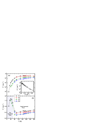
Figure 11: (Color online) Temperature dependence of the ⁷⁷Se NMR (a) spin-lattice $T_{1}^{-1}$ and (b) spin-spin $T_{2}^{-1}$ relaxation rates with the magnetic field of 14.09 T applied parallel to [111]. The inset shows $1/T_{1}$ vs. 1/T for the line P1 and the corresponding fit (solid line) with the contribution from Raman scattering of magnons.

The recovery of the longitudinal magnetization follows, for each peak, a single exponential behavior in time, as expected for a $I=1/2$ nuclear spin. The values of spin-lattice relaxation rate $1/T_{1}$ derived from the fit of the recovery data are shown in Fig. 11(a). At $T>$ 170 K, $1/T_{1}$ varies weakly with temperature for all lines. We may obtain a theoretical fit of $1/T_{1}$ by considering the Raman scattering of magnons off the ⁷⁷Se nuclei which is expected to be the dominant process (at low enough temperatures) that conserves both the total energy and the total angular momentum of the nuclear+electron spin system. To this end, we shall make the reasonable assumption that the relevant lowest spin-wave excitation branch around the minimum $\Delta$ (which is set by the external field) has a typical parabolic dispersion of the form $\epsilon_{\mathbf{k}}=\Delta+\lambda(a\mathbf{k})^{2}$, where $a$ is the lattice constant and $\lambda$ is an energy scale of the order of the actual exchange couplings in the system which gives the curvature around the minimum of the lowest magnon band. Following similar arguments with Refs. [Moriya56, ; Beeman68, ] one obtains

$$\frac{1}{T_{1}}=z\frac{(A/z)^{2}\text{sin}^{2}\theta}{2^{5}\pi^{3}\hbar\lambda}\left(\frac{k_{B}T}{\lambda}\right)^{2}\int_{\Delta/k_{B}T}^{\infty}\frac{dx}{e^{x}-1}$$ (21)

where $z$ is the number of Cu²⁺ ions closest to the nuclear spin, $A/z$ stands for the hyperfine coupling with a single electronic spin, and $\theta$ is the angle between the quantization axes of the electronic and the nuclear spin. Our optimal fit based on a numerical evaluation of the integral of Eq. (21) with $\Delta/k_{B}=g\mu_{B}H$ ($H=14$ T) is shown in the inset of Fig. 11(a) (solid line) and gives $A^{2}\text{sin}^{2}\theta/\lambda^{3}\simeq 1.6\times 10^{7}$ erg^-1. Taking $A/q\sim 2\times 10^{23}$ cm^-3 for the line P1, gives $\lambda/k_{B}\sim 50$ K which is of the right order of magnitude.

Figure 11(b) shows the T-dependence of the spin-spin relaxation rate $1/T_{2}$. These results were obtained by fitting the decay of the spin echo signal $M(2\tau)$, after a $\pi/2-\tau-\pi$ pulse sequence, with the proper functional form. We have found that the decay of the transverse nuclear magnetization follows a single exponential decay in the range 80-290 K while it deviates from the single exponential law below 60 K. The irreversible decay $M(2\tau)$ of the ⁷⁷Se echo signal has the following contributions. First, the ⁷⁷Se nuclear dipole-dipole interaction which can be estimated from the calculation of the van Vleck second momentVleck $M_{2}^{\text{Se-Se}}$ taking into account the natural abundance of ⁷⁷Se.Abragam We have found that $\sqrt{M_{2}^{\text{Se-Se}}}\approx 85s^{-1}$ with a slight variation among the different Se sites, which is much smaller than the experimental values reported in Fig. 11. The second contribution to the spin echo decay is the Redfield term,Slichter96 which is of the form $\text{exp}(-2\tau/T_{1})$. From the $1/T_{1}$ values reported in Fig. 11(a) it is obvious that the contribution of the Redfield term in the spin echo decay is also very small here.

The third contribution to the spin echo decay is due to fluctuating dipolar fields between unlike nuclear spins with the most dominant being the one among Se and Cu nuclei. Depending on the time scale (or correlation time $\tau_{c}$) of these fluctuating dipolar fields we have the following two limiting regimes: (i) The fast motion regime, characterized by $\gamma_{N}\langle\delta H_{z}\rangle\tau_{c}\ll 1$, where the spin echo decay is a single exponential, $\text{exp}(-2\tau/T_{2})$, with $1/T_{2}=\gamma_{N}^{2}\langle\delta H_{z}^{2}\rangle\tau_{c}$,Slichter96 and $\gamma_{N}^{2}\langle\delta H_{z}^{2}\rangle$ is the second moment of the selenium-copper dipolar interaction for which a straightforward lattice sum gives $M_{2}^{\text{Se-Cu}}\simeq 7.7\times 10^{6}s^{-2}$. The fast motion approximation is in our case applicable for $T\gtrsim 80K$. (ii) The quasi-static regime, characterized by $\gamma_{N}\langle\delta H_{z}\rangle\tau_{c}\gg 1$, where the slow fluctuations of the selenium-copper dipolar interaction give rise to a non-exponential spin echo decay. In the nearly static regime the decay goes as $\text{exp}[-(2\tau/T_{2})^{3}]$, where $1/T_{2}=(\gamma_{N}^{2}\langle\delta H_{z}^{2}\rangle/12\tau_{c})^{1/3}$.Takigawa Identifying $\tau_{c}$ with the spin-lattice relaxation time of Cu nuclei, which at 30 K is measured to be about 1ms,T1Cu we find $1/T_{2}\simeq 862~{}s^{-1}$ in agreement with our low-T data. As we noted above the decay of the transverse magnetization is not exponential at low T’s. A good fit of the data can be obtained by both a square exponential decay (half Gaussian) and by a third power exponential. The discrimination between them is prevented by the weakness of the NMR signal at long times.

V Summary

We have presented extensive ⁷⁷Se NMR measurements in single crystals of the magnetoelectric ferrimagnet Cu₂OSeO₃. The analysis of the data has provided a number of central findings both for the crystalline as well as the magnetic phase of this compound. First, the T-dependence of the two types of Cu²⁺ moments, extracted from the NMR data, is fully consistent with a phase transition from the high-T paramagnetic phase to a low-T ferrimagnet whereby 3/4 of the Cu²⁺ moments are aligned parallel and 1/4 antiparallel to the applied field. Below the transition temperature we do not observe any clear change in the broadening of the NMR lines or any splitting of the NMR lines, which shows that there is no measurable symmetry reduction in the crystalline structure from its high-T space group P2₁3. These results are in agreement with previous data from magnetization, high-resolution x-ray, and Neutron diffraction measurements on powder samples reported by Bos et al,Bos but also from infrared,Miller and RamanGnezdilov studies in single crystals of Cu₂OSeO₃.

We have also developed a microscopic spin model with two nearest-neighbor exchange interactions: One antiferromagnetic ($J_{\text{afm}}\simeq 68$ K) between Cu₁ and Cu₂ ions which forces them to be antiparallel to each other, and a second ferromagnetic interaction between nearest-neighbor Cu₂ ions which aligns then in the same direction, giving rise to the above ferrimagnetic state. We have shown that a mean field solution of this model provides a very good description of the physics of the problem and is in excellent agreement with measured magnetization data in a wide temperature range and, more importantly, it is also consistent with the local picture extracted from NMR. A first-principles study of this system may provide a more accurate and refined microscopic spin model.oleg

More generally, our NMR study provides a strong local confirmation that the ferrimagnetic ordering in Cu₂OSeO₃ does not proceed via a spontaneous lattice distortion and thus this material provides a unique example of a metrically cubic crystal that allows for piezoelectric as well as linear magnetoelectric and piezomagnetic coupling.

VI Acknowledgments

We would like to thank K. Schenk, O. Janson, A. Tsirlin, L. Hozoi, and M. Abid for useful discussions. We also acknowledge experimental assistance from K. Schenk, M. Zayed, P. Thomas, and S. Granville. One of the authors (H. B.) acknowledges financial support from the Swiss NSF and by the NCCR MaNEP.

References

- (1) W. Eerenstein, N. D. Mathur, and J. F. Scott, Nature 442, 759 (2006).
- (2) N. A. Spaldin, M. Fiebig, Science 309, 391 (2005).
- (3) D. Khomskii, Physics 2, 20 (2009).
- (4) K. F. Wang, J.-M. Liu, and Z. F. Ren, Advances in Physics 58, 321 (2009).
- (5) L. D. Landau, and E. M. Lifshitz, Electrodynamics of continuous media (Pergamon Press, Oxford, 1984).
- (6) I. E. Dzyaloshinskii, Sov. Phys. JETP 10, 628 (1959).
- (7) M. Gajek, M. Bibes, S. Fusil, K. Bouzehouane, J. Fontcuberta, A. Barthélémy, and A. Fert, Nature Materials 6, 296 (2007).
- (8) V. E. Wood, and A. E. Austin, Int. J. Magn. 5, 303 (1974).
- (9) M. Fiebig, J. Phys. D: Appl. Phys. 38, R123 (2005).
- (10) H. Schmid, Ferroelectrics 162, 317 (1994).
- (11) V. J. Folen, G. T. Rado, and E. W. Stalder, Phys. Rev. Lett. 6, 607 (1961).
- (12) H. Wiegelmann, A. A. Stepanov, I. M. Vitebsky, A. G. M. Jansen, and P. Wyder, Phys. Rev. B 49, 10 039 (1994).
- (13) D. L. Fox, J. F. Scott, J. Phys. C 10, 329 (1977).
- (14) T. Kimura, T. Goto, H. Shintani, K. Ishizaka, T. Arima, and Y. Tokura, Nature 426, 55 (2003).
- (15) N. Hur, S. Park, P. A. Sharma, J. S. Ahn, S. Guha, and S.-W. Cheong, Nature 429, 392 (2004).
- (16) G. Lawes, A. B. Harris, T. Kimura, N. Rogado, R. J. Cava, A. Aharony, O. Entin-Wohlman, T. Yildrim, M. Kenzelmann, C. Broholm, and A. P. Ramirez, Phys. Rev. Lett. 95, 087205 (2005).
- (17) G. Lautenschläger, H. Weitzel, T. Vogt, R. Hock, A. Böhm, M. Bonnet, and H. Fuess, Phys. Rev. B 48, 6087 (1993).
- (18) K. Taniguchi, N. Abe, T. Takenobu, Y. Iwasa, and T. Arima, Phys. Rev. Lett. 97, 097203 (2006).
- (19) Y. J. Choi, H. T. Yi, S. Lee, Q. Huang, V. Kiryukhin, and S.-W. Cheong, Phys. Rev. Lett. 100, 047601 (2008).
- (20) M. Pregelj, O. Zaharko, A. Zorko, Z. Kutnjak, P. Jeglič, P. J. Brown, M. Jagodič, Z. Jagličić, H. Berger, and D. Arčon, Phys. Rev. Lett. 103, 147202 (2009).
- (21) G. Lawes, A. P. Ramirez, C. M. Varma, and M. A. Subramanian, Phys. Rev. Lett. 91, 257208 (2003).
- (22) J-W. G. Bos, C. V. Colin, and T. T. M. Palstra, Phys. Rev. B 78, 094416, (2008).
- (23) K. H. Miller, X. S. Xu, H. Berger, E. S. Knowles, D. J. Arenas, M. W. Meisel, and D. B. Tanner, arXiv:1006.467v1 [cond-mat.mtrl-sci].
- (24) V. P. Gnezdilov, K. V. Lamonova, Yu. G. Pashkevich, P. Lemmens, H. Berger, F. Bussy, and S. L Gnatchenko, Fizika Nizkikh Temperatur 36, 688 (2010).
- (25) H. Effenberger, and F. Pertlik, Monatsh. Chem. 117, 887, (1986).
- (26) A. Larrañaga, J. L. Mesa, L. Lezama, J. L. Pizarro, M. I. Arriortua, and T. Rojo, Materials Research Bulletin, 44, 1, (2009).
- (27) International Tables for Crystallography (2006). Vol. A, ch. 7.1, pp. 610 611 (2006).
- (28) R. M. White, Quantum Theory of Magnetism (McGraw-Hill, New York, 1970).
- (29) A. M. Clogston, and V. Jaccarino, Phys. Rev. 121, 1357 (1960).
- (30) T. Moriya, Prog. Theor. Phys. 16, 23 (1956); 16, 641 (1956).
- (31) D. Beeman and P. Pincus, Phys. Rev. 166, 359 (1968).
- (32) J. V. Vleck, Phys. Rev. 74, 1168 (1948).
- (33) A. Abragam, Principles of Nuclear Magnetism (Oxford University press, 1983).
- (34) C. P. Slichter, Principles of Magnetic Resonance (Springer-Verlag, 1996).
- (35) M. Takigawa, G. Saito, J. Phys. Soc. Jpn. 55, 1233 (1986).
- (36) The copper NMR signal (not shown here) could be observed in Cu2OSeO3 only below 30 K.
- (37) O. Janson, and A. Tsirlin (private communication).