Unitary expansion of the time evolution operator

Abstract

We propose an expansion of the unitary evolution operator, associated to a given Schrödinger equation, in terms of a finite product of explicit unitary operators. In this manner, this unitary expansion can be truncated at the desired level of approximation, as shown in the given examples.

I Introduction

The central problem in any dynamical theory is to find the time evolution of a system that was prepared in a given initial state. In quantum mechanics there are only a few of these problems that are readily solved by simple analytical methods Cohen91 . In general, we have to rely on approximations to obtain out of the Schrödinger equation the time evolution operator $\widehat{U}_{S}(t,t_{0})$ in a suitable form. With the explicit knowledge of $\widehat{U}_{S}(t,t_{0})$, we may calculate the expectation value of any physical observable of the system at any time $t$ once we know the state of system at the time $t_{0}.$ Frequently, we are able to find the time evolution operator $\widehat{U}_{0}(t,t_{0})$ associated with $\widehat{H}_{0}$, a part of the total Hamiltonian $\widehat{H}=\widehat{H}_{0}+\widehat{H}_{\rm int}.$ In this case, it is usually convenient to make a transformation to the “interaction picture” such that

$$\widehat{U}_{S}(t,t_{0})=\widehat{U}_{0}(t,t_{0})\widehat{U}_{I}(t,t_{0})$$ (1)

holds with $\widehat{U}_{0}(t_{0},t_{0})=\widehat{U}_{I}(t_{0},t_{0})=\widehat{I}.$ Consequently, the time evolution operator in the interaction picture, $\widehat{U}_{I}(t,t_{0}),$ satisfies the Schrödinger equation

$$\frac{\partial\widehat{U}_{I}(t,t_{0})}{\partial t}=-i\lambda\widehat{H}_{1}(t)\widehat{U}_{I}(t,t_{0})\,,$$ (2)

where we have considered $\hbar=1$ and have defined $\lambda\widehat{H}_{1}(t)=\widehat{U}_{0}^{\dagger}(t,t_{0})\widehat{H}_{\rm int}(t)\widehat{U}_{0}(t,t_{0}).$ The parameter $\lambda$ is some dimensionless real parameter chosen to give a measure of the relative magnitude of the most important matrix elements of $H_{\rm int}$ and $H_{0}$ in a given problem.

The most popular perturbation approximation method to deal with the Schrödinger equation in Eq. (2) is the Dyson expansion Dyson49 :

$$\widehat{U}_{I}(t,t_{0})=\widehat{I}-i\lambda\int_{0}^{t}dt_{1}\widehat{H}_{1}(t_{1},t_{0})+$$

$${(-i\lambda)^{2}}\int_{0}^{t}dt_{1}\int_{0}^{t_{1}}dt_{2}\widehat{H}_{1}(t_{1},t_{0})\widehat{H}_{1}(t_{2},t_{0})+...\,,$$ (3)

where it is very convenient to estimate the solution by truncating the series to a given order $\lambda^{n}$. Besides the normal difficulties to calculate high-order terms, the Dyson truncation produces an approximated evolution operator that is not unitary. Other expansions of operator $\widehat{U}_{1}(t,t_{0})$ have also been proposed in the literature, as the Magnus expansion Magnus54 the Fer product Fer58 and, more recently, the Aniello expansion Aniello05 . New bounds for the convergence of the Magnus expansion and the Fer product have been recently studied in Ref. Blanes98 . Other product expansions have also been considered in the literature see .

In this paper, we present an alternative method to calculate the time evolution operator $U_{I}(t,t_{0})$ as a product of a finite number of unitary operators

$$\widehat{U}_{I}(t,t_{0})=\widehat{U}_{1}(t,t_{0})\widehat{U}_{2}(t,t_{0})\cdots\widehat{U}_{k}(t,t_{0})\cdots\widehat{U}_{N}(t,t_{0})\,,$$ (4)

where each operator $\widehat{U}_{k}(t,t_{0}),k=1,2,...N-1$, can be written as the exponential of an anti-Hermitian operator proportional to $(\lambda)^{k}$, while $\widehat{U}_{N}(t,t_{0})-\widehat{I}$ is at most of order $(\lambda)^{N}$. The number $N$ of operators in the expansion can be as large as we want. If we approximate the last operator $\widehat{U}_{N}(t,t_{0})$ in the product by the unit operator, we obtain an expansion of the evolution operator $\widehat{U}_{I}(t,t_{0})$ which is explicitly unitary to order $(\lambda)^{N-1}$. Besides this important advantage, this expansion is well suited to treat a variety of problems. In Section II, we derive the expressions for each term in the expansion; in Section III, we provide pedagogical examples; and in Section IV, we present our conclusions.

II The method

We start with the simple case of $N=2.$ Equation (4) can then be written as

$$\widehat{U}_{I}(t,t_{0})=\widehat{U}_{1}(t,t_{0})\widehat{U}_{2}(t,t_{0}).$$ (5)

Following the same kind of procedure used in the transformation to the interaction representation, we write

$$\widehat{U}_{I}(t,t_{0})=e^{-i\lambda\widehat{W}_{1}(t,t_{0})}\widehat{U}_{2}(t,t_{0})\,,$$ (6)

where $\widehat{W}_{1}(t,t_{0})$ is an hermitian operator to be chosen conveniently. From now on, we set $t_{0}=0$ and avoid writing it to simplify the notation. From Eqs. (2), (5) and (6), we have

$$\frac{\partial\widehat{U}_{2}(t)}{\partial t}=-i\lambda\widehat{H}_{2}(t)\widehat{U}_{2}(t)\,,$$ (7)

where

$$\widehat{H}_{2}(t)\!=\!\sum_{m=0}^{\infty}\frac{(i\lambda)^{m}}{m!}(ad\hskip 1.42271pt\widehat{W}_{1}(t))^{m}\Big{\{}\widehat{H}_{1}(t)-\frac{1}{m+1}\frac{\partial\widehat{W}_{1}(t)}{\partial t}\Big{\}}.$$

Here, we have defined $ad\widehat{A}\{\cdot\}=[\widehat{A},\cdot]$ and used the following relation

$$e^{\alpha\widehat{A}}\widehat{B}e^{-\alpha\widehat{A}} = \sum_{m=0}^{\infty}\frac{\alpha^{m}}{m!}(ad\hskip 1.42271pt\widehat{A})^{m}\big{\{}\widehat{B}\big{\}}$$ (9)

$$= \widehat{B}+\alpha[\widehat{A},\widehat{B}]+\frac{\alpha^{2}}{2!}[\widehat{A},[\widehat{A},\widehat{B}]]+\cdots$$

Choosing

$$\widehat{W}_{1}(t)=\int_{0}^{t}\widehat{H}_{1}(t^{\prime})dt^{\prime}\,,$$ (10)

we have

$$\widehat{H}_{2}(t)=\sum_{m=1}^{\infty}\frac{(i\lambda)^{m}}{(m+1)!}(ad\hskip 1.42271pt\widehat{W}_{1}(t))^{m}\big{\{}m\widehat{H}_{1}(t)\big{\}}\,,$$ (11)

which is of order $\lambda$. In this case, $\widehat{U}_{2}(t)$ is the solution of Eq. (7) and should be written as an exponential of a non-Hermitian operator that is, in general, a series on the variable $\lambda$, starting with $\lambda^{2}.$

In the simple case where $[\widehat{H}_{1}(t),\widetilde{H}_{1}(t^{\prime})]=-2if(t,t^{\prime})$ is a c-number function, then

$$\widehat{H}_{2}(t)=\lambda\int_{0}^{t}dt^{\prime}f(t^{\prime},t)$$ (12)

is also a c-number function. Consequently, Eq. (7) can be easily integrated to give $\widehat{U}_{2}(t)=e^{-i\lambda^{2}\phi(t)}$, where

$$\phi(t)=\int_{0}^{t}dt^{\prime}\int_{0}^{t^{\prime}}dt^{\prime\prime}f(t^{\prime\prime},t^{\prime})$$ (13)

and the time evolution operator is

$$\widehat{U}_{I}(t)=e^{-i\lambda\int_{0}^{t}dt_{1}\widehat{H}_{1}(t_{1})}e^{-i\lambda^{2}\phi(t)}.$$ (14)

This result is well known and could also be easily obtained using the Magnus expansion Pechugas66 . It can be used, for example, to easily obtain the time evolution operator for the quantum state generated by an external time-dependent force acting on a mechanical oscillator, as we show in the next section.

The procedure described above can be generalized for any value of $N$ greater than $2$ by setting

$$\widehat{U}_{n}(t)=e^{-i\lambda\widehat{W}_{n}(t)}\widehat{U}_{n+1}(t)\,,n=2,3...N-1\,,$$ (15)

so that expansion of the operator $\widehat{U}_{I}(t)$ may also read

$$\widehat{U}_{I}(t)=e^{-i\lambda\widehat{W}_{1}(t)}e^{-i\lambda\widehat{W}_{2}(t)}...e^{-i\lambda\widehat{W}_{N-1}(t)}\widehat{U}_{N}(t).$$ (16)

The operators $\widehat{U}_{n}(t),$ for $n=2,3..$ satisfy a Schrödinger-like equation

$$\frac{\partial\widehat{U}_{n}(t)}{\partial t}=-i\lambda\widehat{H}_{n}(t)\widehat{U}_{n}(t)\,,$$ (17)

where $\widehat{H}_{n}(t)$ is given by

$$\widehat{H}_{n}(t) = \sum_{m=0}^{\infty}\frac{(i\lambda)^{m}}{m!}(ad\hskip 1.42271pt\widehat{W}_{n-1}(t))^{m}$$ (18)

$$\times\Big{\{}\widehat{H}_{n-1}(t)-\frac{1}{m+1}\frac{\partial\widehat{W}_{n-1}(t)}{\partial t}\Big{\}}\,.$$

By choosing operators $\widehat{W}_{j}(t)$’s for $j=1,...N-1,$ we obtain operators $\widehat{H}_{j}(t)$ for $j=2,...N$, and the expansion given by Eq. (16).

We now show that it is possible to choose operators $\widehat{W}_{n}(t)$ being proportional to $\lambda^{n-1}$, and such that the operators $\widehat{H}_{n}(t)$ are power series in the variable $\lambda$ starting with the power $\lambda^{n-1}.$ Then, by substituting $\widehat{W}_{n}(t),n=1,2...(N-1)$ in Eq. (4) and noticing that $\widehat{I}-\widehat{U}_{N}(t)$ would be at least of ${\cal{O}}(\lambda^{N}),$ we will obtain the desired expansion announced in the Introduction. We make the proof by construction. Writing explicitly the dependence of the operators $\widehat{W}_{n}(t)$ and $\widehat{H}_{k}(t)$ on $\alpha=i\lambda$, we have

$$\widehat{W}_{k}(t) = \alpha^{k-1}\widetilde{W}_{k}(t)\,,$$

$$\widehat{H}_{k}(t) = \sum_{j=k-1}^{\infty}\widetilde{H}_{k,j}(t)\alpha^{j}.$$ (19)

By substituting Eq. (II) in Eq. (18) we get, for $j\geq n\geq 1,$

$$\widetilde{H}_{n+1,j}=\sum_{m=1}^{\infty}\sum_{k=1}^{n}\sum_{i=k-1}^{\infty}\frac{1}{m!}(ad\widetilde{W}_{k}(t\hskip 1.42271pt))^{m}\Big{\{}\widetilde{H}_{k,i}\delta(km+i-j)\Big{\}}-\sum_{k=1}^{n}\sum_{m=0}^{\infty}\frac{1}{(m+1)!}(ad\widetilde{W}_{k}(t)\hskip 1.42271pt)^{m}\Big{\{}\frac{d\widetilde{W}_{k}(t)}{dt}\delta(km+k-1-j)\Big{\}}\,,$$ (20)

and for $0<j<n,$

$$\frac{d\widetilde{W}_{j+1}(t)}{dt}=\sum_{m=1}^{\infty}\sum_{k=1}^{n}\sum_{i=k-1}^{\infty}\frac{1}{m!}(ad\widetilde{W}_{k}(t)\hskip 1.42271pt)^{m}\Big{\{}\widetilde{H}_{k,i}\delta(km+i-j)\Big{\}}-\sum_{k=1}^{n}\sum_{m=1}^{\infty}\frac{1}{(m+1)!}(ad\widetilde{W}_{k}(t)\hskip 1.42271pt)^{m}\Big{\{}\frac{d\widetilde{W}_{k}(t)}{dt}\delta(km+k-1-j)\Big{\}}\,,$$ (21)

where $\delta(m-n)=\delta_{m,n}$ is the Kronecker delta. Notice that $j+1{>}k$ in Eq. (21) so that $\frac{d\widetilde{W}_{j+1}(t)}{dt}$ is given recursively in terms of the operators $\widetilde{W}_{k}(t)$ and $\widetilde{H}_{k}(t),$ for $k\leq j$. For example, if we set $n=2$ and $j=1$ in the above equations, we easily get

$$\frac{d\widetilde{W}_{2}(t)}{dt} = \frac{1}{2}(ad\widetilde{W}_{1}(t)\hskip 1.42271pt)\big{\{}\widehat{H}_{1}(t)\big{\}}\,,$$ (22)

where we used Eq. (21) and the fact that $\widetilde{H}_{1,0}(t)=\widehat{H}_{1}(t).$ Using the initial condition $\widehat{W}_{2}(0)=0,$ we have

$$\widetilde{W}_{2}(t) = \frac{1}{2}\int_{0}^{t}dt^{\prime}[\widetilde{W}_{1}(t^{\prime}\hskip 1.42271pt),\widehat{H}_{1}(t^{\prime})]\,,$$ (23)

which also can be written as

$$\widetilde{W}_{2}(t)=\frac{1}{2}\int_{0}^{t}dt_{1}\int_{0}^{t_{1}}dt_{2}[\widehat{H}_{1}(t_{2}),\widehat{H}_{1}(t_{1})]\,.$$ (24)

To obtain an approximate expression for $\widehat{U}_{I}(t)$ valid to order O$(\lambda^{2}),$ we first set $N=3$ in Eq (16):

$$\widehat{U}_{I}(t)=e^{-i\lambda\widetilde{W}_{1}(t)}e^{-(i\lambda)^{2}\widetilde{W}_{2}(t)}\widehat{U}_{3}(t)\,.$$ (25)

$\widehat{U}_{3}(t)-\widehat{I}$ is of order $\lambda^{3},$ since it satisfies the Schrödinger equation, Eq. (17), with $\widehat{H}_{3}(t)$ of the order O$(\lambda^{2}).$ If we approximate $\widehat{U}_{3}(t)$ by the identity we get an approximation which is unitary and valid to order ${\cal O}(\lambda^{2}).$ Using the expressions for $\widetilde{W}_{1}(t)=\widehat{W}_{1}(t)$ and for $\widetilde{W}_{2}(t)$ given in Eq. (10) and Eq. (23), we have

$$\widehat{U}_{I}(t)\approx\exp\{(-i\lambda)\int_{0}^{t}dt_{1}\widetilde{H}_{1}(t_{1})\}\times$$

$$\exp\{\frac{\lambda^{2}}{2}\int_{0}^{t}dt_{1}\int_{0}^{t_{1}}dt_{2}[\widehat{H}_{1}(t_{2}),\widehat{H}_{1}(t_{1})]\}\,.$$ (26)

The procedure described above can be generalized for obtaining approximations involving a product of $N$ operators, by calculating $\widetilde{W}_{k}(t),k=1,...N,$ through Eqs. (20) and (21). Below we give, as examples, the explicit expressions for $\widetilde{W}_{3}(t),$ $\widetilde{W}_{4}(t),$ and $\widetilde{W}_{5}(t)$

$$\widetilde{W}_{3}(t) = \frac{1}{3}\int_{0}^{t}dt^{\prime}[\widetilde{W}_{1}(t^{\prime}),[\widetilde{W}_{1}(t^{\prime}),\widetilde{H}_{1}(t^{\prime})]]\,,$$

$$\widetilde{W}_{4}(t) = \frac{3}{4!}\int_{0}^{t}dt^{\prime}[\widetilde{W}_{1}(t^{\prime}),[\widetilde{W}_{1}(t^{\prime}),[\widetilde{W}_{1}(t^{\prime}),\widetilde{H}_{1}(t^{\prime})]]]$$

$$+ \frac{1}{4}\int_{0}^{t}dt^{\prime}[\widetilde{W}_{2}(t^{\prime}),[\widetilde{W}_{1}(t^{\prime}),\widetilde{H}_{1}(t^{\prime})]]\,,$$

$$\widetilde{W}_{5}(t) = \frac{4}{5!}\int_{0}^{t}dt^{\prime}[\widetilde{W}_{1}(t^{\prime}),$$ (27)

$$[\widetilde{W}_{1}(t^{\prime}),[\widetilde{W}_{1}(t^{\prime}),[\widetilde{W}_{1}(t^{\prime}),\widetilde{H}_{1}(t^{\prime})]]]]$$

$$+ \frac{2}{3!}[\widetilde{W}_{2}(t^{\prime}),[\widetilde{W}_{1}(t^{\prime}),[\widetilde{W}_{1}(t^{\prime}),\widetilde{H}_{1}(t^{\prime})]]].$$

As we show in the next section, the expansion obtained above may be useful in several cases and in particular for obtaining effective time independent hamiltonians, when the operator $\widehat{U}_{n}(t^{\prime})$ in the expansion can be approximated by the exponential of the product of the time with a constant operator.

Notice that besides the fact that they are Hermitian, no restriction was made on the operators $\widehat{W}_{n}(t)$ for $n=2,3...$ until now. Special choices of $\widehat{W}_{n}(t),$ other than the one we have chosen to discuss in this paper, may lead to interesting applications in specific cases.

III Examples of applications

In this section we describe three examples of applications of the method: i) the problem of a linear harmonic oscillator subjected to a driving force; ii) the Raman resonant transition inside a cavity; iii) the ultrastrong coupling (USC) and deep strong coupling (DSC) regimes of the Jaynes-Cummings (JC) model.

We start with the well known problem of a linear harmonic oscillator subject to a driving force $-gf(t).$ The Hamiltonian is given by $(\hbar=1)$

$$H=\omega(\widehat{a}^{\dagger}\widehat{a}+1/2)+gf(t)(\widehat{a}+\widehat{a}^{\dagger})$$ (28)

where $\widehat{a}$ and $\widehat{a}^{\dagger}$ are the usual annhilation and creation operators satisfying the algebra $[\widehat{a},\widehat{a}^{\dagger}]=1.$

We first take $H_{0}=\omega(\widehat{a}^{\dagger}\widehat{a}+1/2)$ and go to the interaction representation by defining $\widehat{U}(t)=e^{-i\widehat{H}_{0}t/\hbar}\widehat{U}_{1}(t)$, where

$$\frac{\partial\widehat{U}_{1}(t)}{\partial t}=-ig\widehat{H}_{1}(t)\widehat{U}_{I}(t)\,,$$ (29)

with

$$\widehat{H}_{1}(t)=f(t)(\widehat{a}e^{-i\omega t}+\widehat{a}^{\dagger}e^{i\omega t}).$$ (30)

In this case, $[\widehat{H}_{1}(t),\widehat{H}_{1}(t^{\prime})]=-2if(t)f(t^{\prime})\sin{\omega(t-t^{\prime})}$ is a c-number. Therefore, $\widehat{W}_{n}=0$ for $n>2,$ $\widehat{U}_{3}=\widehat{I},$ and

$$\widetilde{W}_{1}(t) = \int_{0}^{t}dt^{\prime}f(t^{\prime})(\widehat{a}e^{-i\omega t^{\prime}}+\widehat{a}^{\dagger}e^{i\omega t^{\prime}}),$$ (31)

$$\widetilde{W_{2}}(t) = i\int_{0}^{t}dt_{1}\int_{0}^{t_{1}}dt_{2}f(t_{1})f(t_{2})\sin{\omega(t_{1}-t_{2})}.$$

Then, the time evolution operator in the interaction picture is given by

$$\widehat{U}_{1}(t)=e^{i\varphi(t)}\widehat{D}(v(t))$$ (32)

where $\varphi(t)=g^{2}\widetilde{W}_{2}(t)$ is a time-dependent phase and $\widehat{D}(v(t))=e^{v(t)\widehat{a}^{\dagger}-v^{*}(t)\widehat{a}}$ is the displacement operator and

$$v(t)=-ig\int_{0}^{t}dt^{\prime}f(t^{\prime})e^{i\omega t^{\prime}}.$$ (33)

Another example is the case of resonant Raman scattering inside a cavity. Consider a three-level $\Lambda$ atom interacting quasi-resonantly with a mode of frequency $\omega_{1}$ of the cavity field and a classical field of frequency $\omega_{2}$, as schematized in Fig (1). The two lower levels, $|g\rangle$ and $|e\rangle,$ are closely spaced in energy and can make quasi-resonant dipole transitions to an upper level $|i\rangle.$ $\omega_{ig}$ and $\omega_{ie}$ are the energy differences between the upper level and the lower levels $|g\rangle$ and $|e\rangle,$ respectively. The Hamiltonian that describes the interaction in the rotating-wave approximation is given by

$$\widehat{H} = \widehat{H}_{0}^{\prime}+\widehat{H}_{\rm int}^{\prime}$$

$$\widehat{H}_{0}^{\prime} = \omega_{ig}|{i}\rangle\langle{i}|+\omega_{eg}|{e}\rangle\langle{e}|+\omega_{1}\widehat{a}^{\dagger}\widehat{a}$$

$$\widehat{H}_{\rm int}^{\prime} = \Omega_{ig}|{i}\rangle\langle{g}|\widehat{a}+\Omega_{ie}e^{-i\omega_{2}t}|{i}\rangle\langle{e}|$$ (34)

$$+ \Omega_{ig}|{g}\rangle\langle{i}|\widehat{a}^{\dagger}+\Omega_{ie}e^{i\omega_{2}t}|{e}\rangle\langle{i}|,$$

where $\Omega_{ig}$ is the vacuum Rabi frequency associated to the cavity field of frequency $\omega_{1}$, while $\Omega_{ie}$ is the Rabi frequency associated to the external classical field of frequency $\omega_{2}$. Assume that the initial cavity field state has a photon distribution with low photon average number. In Ref. Franca01 , it has been shown that if the detuning $\delta=\omega_{ig}-\omega_{1}\approx\omega_{ig}-\omega_{eg}-\omega_{2}$ is such that $|\delta|\gg\Omega_{gi}\gg\Omega_{ei}$, it is then possible to show that the Raman transition $|g,n_{0}+1\rangle\leftrightarrow|e,n_{0}\rangle$ is resonant for a certain $n_{0}$ depending on the detunings of the driving field. Here we rederive the conditions on the frequencies that make the process resonant and the effective hamiltonian for the system.

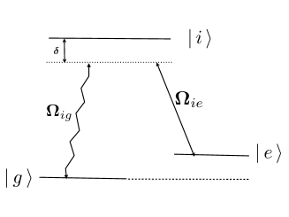
Figure 1: Raman transition of a $\Lambda$ atom inside a cavity.

Assume that the classical field frequency is tuned to

$$\omega_{2}=\omega_{1}-\omega_{eg}-(n_{0}+1)\Omega_{gi}^{2}/\Delta+\Omega_{ei}^{2}/\Delta,$$ (35)

with $\Delta$ satisfying the equation

$$\Delta=\omega_{ig}-\omega_{1}+(\Omega_{ei}^{2}+2\Omega_{gi}^{2})/\Delta+2n_{0}{\Omega_{gi}^{2}}/{\Delta},$$ (36)

where $n_{0}$ is an integer and $|\Delta|\gg\Omega_{gi}\gg\Omega_{ei}.$

We first write the Hamiltonian of Eq. (III) as $\widehat{H}=\widehat{H}_{0}+\widehat{H}_{\rm int}$ with

$$\widehat{H}_{0} = \widehat{H}_{0}^{\prime}+\widehat{H}_{SS}$$

$$\widehat{H}_{\rm int} = \widehat{H}_{\rm int}^{\prime}-\widehat{H}_{SS},$$ (37)

where $\widehat{H}_{0}^{\prime}$ and $\widehat{H}_{\rm int}^{\prime}$ are given by Eq. (III). Also, $\widehat{H}_{\rm SS}$ is given by

$$\widehat{H}_{\rm SS}=(\frac{\Omega_{gi}^{2}}{\widehat{\Delta}_{g}}\widehat{a}\widehat{a}^{\dagger}+\frac{\Omega_{ei}^{2}}{\widehat{\Delta}_{e}})|{i}\rangle\langle{i}|-\frac{\Omega_{gi}^{2}}{\widehat{\Delta}_{g}}\widehat{a}^{\dagger}\widehat{a}|{g}\rangle\langle{g}|-\frac{\Omega_{ei}^{2}}{\widehat{\Delta}_{e}}|{e}\rangle\langle{e}|\,,$$ (38)

where

$$\widehat{\Delta}_{g} = \omega_{1}-\omega_{ig}+{\Omega_{ig}^{2}(2\widehat{n}+1)}/{\Delta}$$

$$\widehat{\Delta}_{e} = \omega_{2}-\omega_{ie}+{\Omega_{ie}^{2}\widehat{n}}/{\Delta}\,.$$ (39)

We then write the time evolution operator in the interaction representation with respect to $\widehat{H}_{0}$ and use our unitary perturbative expansion. Neglecting terms that vary very rapidly with time, we obtain

$$\lambda\widehat{W}_{1} = -\widehat{H}_{SS}t$$

$$\lambda\widehat{W}_{2} = \widehat{H}_{SS}+\widehat{H}_{\rm eff}t\,,$$ (40)

where

$$\widehat{H}_{\rm eff}=-\frac{\Omega_{gi}\Omega_{ei}}{\Delta}(|e\rangle\langle g|\widehat{a}+|g\rangle\langle e|\widehat{a}^{\dagger}).$$ (41)

Therefore

$$\widehat{U}_{I}(t)\approx e^{+i\widehat{H}_{SS}t}e^{-i(\widehat{H}_{SS}+\widehat{H}_{\rm eff})t}\,.$$ (42)

Using the Baker-Hausdorff formula and neglecting the term depending on the commutators of $\widehat{H}_{SS}$ and $\widehat{H}_{\rm eff},$ we may write

$$\widehat{U}_{I}(t,0)\approx e^{-i\widehat{H}_{\rm eff}t}.$$ (43)

That is, $\widehat{H}_{\rm eff}$ can be considered an effective Hamiltonian of the interaction picture associated to the choice of $\widehat{H}_{0}$ given in the Eq. (III).

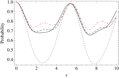
Figure 2: Survival probability of $|g;0\rangle$ vs. $\tau=\omega t.$ Solid line: exact solution; dashed line: $\widehat{U}\approx\widehat{U}_{0}\widehat{U}_{1};$ dot dashed line, first Born approx.; dotted line $\widehat{U}\approx\widehat{U}_{0}.$ $\omega_{0}/\omega=0.6;g/\omega=0.5.$

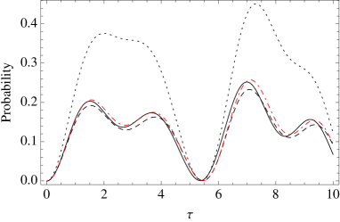
Figure 3: Probability of $|g;0\rangle$ to make a transition to the state $|e;1\rangle$ as a function of $\tau=\omega t.$ Solid line: exact solution; dashed line: $\widehat{U}\approx\widehat{U}_{0}\widehat{U}_{1};$ dot dashed line: first Born approximation; dotted line $\widehat{U}\approx\widehat{U}_{0}.$ $\omega_{0}/\omega=0.6;g/\omega=0.5.$

Consider now the situation of the Jaynes-Cummings model in the USC regime between a cavity mode and a qubit, $g/\omega\gtrsim 0.1$. This situation is currently accessible to experiments using superconducting qubits and cavities in circuit quantum electrodynamics Niemczyk10 ; Forn-Diaz10 . In this case, the rotating-wave approximation is no longer valid and one should consider the full interaction Hamiltonian

$$\widehat{H}=\omega\widehat{a}^{\dagger}\widehat{a}+g(\widehat{a}^{\dagger}+\widehat{a})\widehat{\sigma}_{x}+\omega_{0}\widehat{\sigma}_{z}/2\,.$$ (44)

In the case where $\omega_{0}=0$, it reduces to

$$\widehat{H}^{\prime}=\omega\widehat{a}^{\dagger}\widehat{a}+g(\widehat{a}^{\dagger}+\widehat{a})\widehat{\sigma}_{x}\,.$$ (45)

The eigenstates of $\widehat{H}^{\prime}$ are the product of displaced number states Oliveira90 and the eigenstates $|\pm\rangle$ of $\widehat{\sigma}_{x}$, associated with the eigenvalues $\pm 1$

$$|\pm n;\pm\rangle=\widehat{D}(\mp x)|n\rangle\otimes|\pm\rangle,$$ (46)

where $x=g/\omega$, $\widehat{D}(v)=e^{v\widehat{a}^{\dagger}-v^{*}\widehat{a}}$ is the displacement operator, $|n\rangle,n=0,1,2..$ are Fock states, and $\widehat{\sigma}_{x}|\pm\rangle=\pm|\pm\rangle.$ The eigenstates $\widehat{D}(\mp x)|n\rangle$ of $\widehat{H}^{\prime}$ are degenerated and associated with the eigenvalue $(n\omega-g^{2}/\omega).$

In basis $\{|\pm n;\pm\rangle,n=0,1,...\}$, $\omega_{0}\widehat{\sigma}_{z}/2$ is written as

$$\omega_{0}\widehat{\sigma}_{z}/2=\omega_{0}/2\sum_{n,m}\langle n|\widehat{D}(2x)|m\rangle\,\,|+n;+\rangle\langle-m;-|+{\rm H.c.}$$ (47)

In Ref. Irish05 , it has been proposed an approximation which keeps only the terms with $n=m$ in the right hand side of Eq. (47), that is,

$$\widehat{H}_{0}=\widehat{H}^{\prime}+\omega_{0}/2\sum_{n}\langle n|\widehat{D}(2x)|n\rangle\,\,|+n;+\rangle\langle-n;-|+{\rm H.c.},$$ (48)

where $\langle n|\widehat{D}(2x)|n\rangle=e^{-2x^{2}}{\cal L}_{n}(4x^{2}).$ The eigenstates of $\widehat{H}_{0}$ can be easily written as

$$\frac{1}{\sqrt{2}}(|+n;+\rangle\pm|-n;-\rangle\,,$$ (49)

and are associated to the eigenvalues $n\omega-g^{2}/\omega\pm(\omega_{0}/2)\langle n|\widehat{D}(2x)|n\rangle.$

Using the approximate Hamiltonian $\widehat{H}_{0}$ as our zeroth-order approximation, we have found that our method is well suited for describing transition probabilities for a very large range of $\omega_{0}/\omega$ and $g/\omega\gtrsim 0.1$, including both, the USC and DSC regimes of the JC model Casanova10 . Let us write $\widehat{H}=\widehat{H}_{0}+\widehat{H}_{\rm int}$, where

$$\widehat{H}_{\rm int}=\omega_{0}/2\sum_{n\neq m}\langle n|\widehat{D}(2x)|m\rangle\,\,|+n;+\rangle\langle-m;-|+{\rm H.c.}$$ (50)

From Eqs. (48) and (50) we can easily calculate $\lambda\widehat{H}_{1}(t)=e^{i\widehat{H}_{0}t}\widehat{H}_{\rm int}e^{-i\widehat{H}_{0}t}$ and the operators $\widehat{W}_{1}$ and $\widehat{W}_{2}$ using the expressions given in Eqs. (10) and (23).

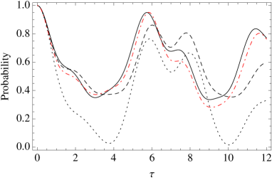
Figure 4: Survival probability of $|g;0\rangle$ as a function of $\tau=\omega t.$ Solid line: exact solution; dashed line: $\widehat{U}\approx e^{-i\widehat{H}_{0}t}e^{-i\lambda\widehat{W}_{1}(t)};$ dot dashed line: $\widehat{U}\approx e^{-i\widehat{H}_{0}t}e^{-i\lambda\widehat{W}_{1}(t)}e^{-i\lambda\widehat{W}_{2}(t)};$ dotted line $\widehat{U}\approx e^{-i\widehat{H}_{0}t}.$ $\omega_{0}/\omega=1;g/\omega=0.8.$

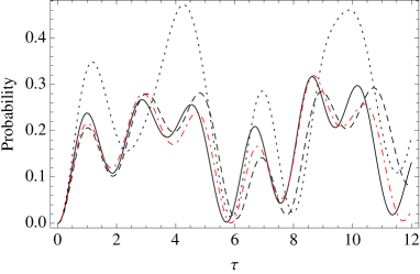
Figure 5: Transition probability from $|g;0\rangle$ to $|e;1\rangle$ vs. $\tau=\omega t.$ Solid line: exact solution; dashed line: $\widehat{U}\approx\widehat{U}_{0}\widehat{U}_{1};$ dot dashed line: $\widehat{U}\approx\widehat{U}_{0}\widehat{U}_{1}\widehat{U}_{2}$; dotted line $\widehat{U}\approx\widehat{U}_{0}.$ $\omega_{0}/\omega=1;g/\omega=0.8.$

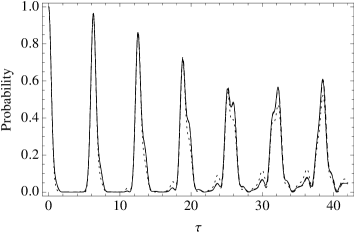
Figure 6: Survival probability of $|g;0\rangle$ as a function of $\tau=\omega t.$ Solid line: exact solution is superposed with $\widehat{U}\approx\widehat{U}_{0}\widehat{U}_{1};$ dotted line $\widehat{U}\approx\widehat{U}_{0}.$ $\omega_{0}/\omega=0.5;g/\omega=2.$

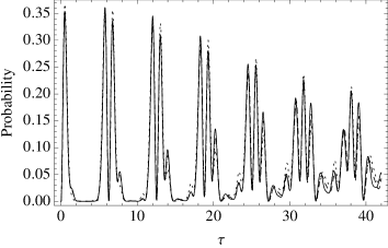
Figure 7: Probability of $|g;0\rangle$ to make a transition to $|e;1\rangle$ as a function of $\tau=\omega t.$ Solid line: exact solution is superposed with $\widehat{U}\approx\widehat{U}_{0}\widehat{U}_{1};$ dotted line $\widehat{U}\approx\widehat{U}_{0}.$ $\omega_{0}/\omega=0.5;g/\omega=2.$

In Figs. 2 and 3, we present curves corresponding to the exact result calculated numerically, the results calculated using three approximations for the time evolution operator: $e^{-i\widehat{H}_{0}t},$ $e^{-i\widehat{H}_{0}t}e^{-i\lambda\widehat{W}_{1}(t)},$ and the Dyson approximation to first order in $\omega_{0}$. The results show that both, the approximation $\widehat{H}=\widehat{H}_{0}$ and the first Born approximation, do not describe the transition probabilities for the USC regime. On the other hand, our unitary expansion describes quite well the results, even when we take only the first non-trivial contribution. Note that the contribution of $\widehat{W}_{2}$ is not shown and gives a small correction.

In Figs. 4 and 5, we also present curves corresponding to the exact result calculated numerically and those calculated using three approximations for the time evolution operator: $e^{-i\widehat{H}_{0}t},$ $e^{-i\widehat{H}_{0}t}e^{-i\lambda\widehat{W}_{1}(t)}$ and $e^{-i\widehat{H}_{0}t}e^{-i\lambda\widehat{W}_{1}(t)}e^{-i\lambda\widehat{W}_{2}(t)}.$ The first Born approximation is not shown and represents a small correction to the approximation $\widehat{H}\approx\widehat{H}_{0}.$ We see that, although the terms associated with $\widehat{W}_{1}$ gives the main contribution, the terms associated with $\widehat{W}_{2}$ does improve the approximation. These considerations are also applicable to the DSC regime Casanova10 , as can be seen in Figs. 6 and 7.

IV Conclusions

We introduced a perturbative unitary expansion for the time evolution operator as a product of exponentials of antihermitian operators. Consequently, this expansion can be truncated at any order of approximation while keeping unitarity. We have presented three examples: a harmonic oscillator with a time-dependent force, the Raman transition inside a resonant cavity, and the James-Cummings model in the USC and DSC regimes.