Applicability of the hydrodynamic description of classical fluids

Abstract

We investigate using numerical simulations the domain of applicability of the hydrodynamic description of classical fluids at and near equilibrium. We find this to be independent of the degree of many-body correlations in the system; the range $r_{c}$ of the microscopic interactions completely determines the maximum wavenumber $k_{max}$ at which the hydrodynamic description is applicable by $k_{max}r_{c}\simeq 0.43$. For the important special case of the Coulomb potential of infinite range, we show that the ordinary hydrodynamic description is never valid.

The equations of hydrodynamics Landau , such as the Navier-Stokes equations, are certainly the most widely used framework for investigating the dynamics of fluids, including gases Mansour , liquids Scopigno , plasmas Gedalin and nuclear matter Bouras . Despite widespread use and successes, a number of outstanding questions of both fundamental and practical importance remain regarding the conditions under which the hydrodynamic description holds.

One ordinarily thinks of the hydrodynamic picture as applying only for wavenumbers $k$ such that $kl_{f}\ll 1$ with $l_{f}$ the mean free path and frequencies $\omega$ such that $\omega/\omega_{c}\ll 1$ with $\omega_{c}$ the mean collision frequency. These conditions, derived and already rather qualitative for a system governed by uncorrelated binary collisions (e.g. a dilute gas), become even more indeterminate when many-body correlations are present (as is the case, for example, in a liquid) because the concepts of mean free path and mean collision time cease to have a clear physical meaning. Thus the applicability of the hydrodynamic description certainly depends strongly on the thermodynamic conditions - e.g. the density $n$ and temperature $T$ - as well as the strength and range of the particles’ mutual interactions. For instance, one expects that the description never applies on lengthscales smaller than the range $r_{c}$ of the potential (i.e. $kr_{c}\gtrsim 1$) – in other words, that the domain of validity will shrink as the range increases (such long range potentials are of particular importance in plasma physics). In fact, in the extreme case of $r_{c}=\infty$, the very existence of a hydrodynamic description is a known but unsolved problem BausHansen . As well as leading to a deeper understanding of the emergence of macroscopic behaviour in interacting many-body systems, it is also of significant practical importance to know exactly when hydrodynamics can be used to describe the behaviour of fluids, e.g. for analysing light and neutron scattering experiments Scopigno ; BalucaniZoppi ; Glenzer .

In this Letter, we address with numerical simulations the question of the domain of applicability of the hydrodynamic description for fluids at or near equilibrium as the level of many-body correlations in the system is varied. To this end, we consider a one-component system with a Yukawa interaction potential $v(r)=q^{2}\exp(-r/r_{c})/r$, where $q^{2}$ is the strength and $r_{c}$ the range of the potential. Although not possessing the short range features of conventional pair potentials used to describe normal liquids, the Yukawa potential is certainly suitable for investigating the long lengthscale dynamics that concern the hydrodynamic description. Additionally, it is commonly used in describing the screened interactions in plasmas Donkorev ; SaizWunsch . What is more, since for $r_{c}=\infty$ one recovers the Coulomb potential, we are able to use this model to answer the question of the existence of the hydrodynamic limit referred to previously. Most importantly however, this model is very convenient here because it is known to be fully characterised by two dimensionless parameters only Donkorev - the reduced range $r_{c}^{*}=r_{c}/a$, where $a=\left(4\pi\/n/3\right)^{-1/3}$ is the average inter-particle spacing, and the coupling strength $\Gamma=q^{2}/(ak_{b}T)$, which itself characterises completely the degree of many-body correlations present in the system for a given range Ichimaru . For a wide range of $\Gamma$ and $r_{c}^{*}$ values, thus spanning states ranging from dilute gases to dense liquids Daligault , with short or long range microscopic interactions, we determine the length and time scales at which the hydrodynamic description breaks down.

To accomplish this, we have computed with Molecular Dynamics (MD) simulations the dynamical structure factor, $S(k,\omega)$, that is the Fourier transform in space and time of the density autocorrelation function, for a wide range of $\Gamma$ ($0.1$,$1$,$5$,$10$,$50$,$120$,$175$) and $r_{c}^{*}$ ($0.5$,$1$,$1.4$,$2$,$3.3$,$10$,$\infty$) values. $S(k,w)$ contains complete information of the system dynamics at and near thermal equilibrium through the Fluctuation-Dissipation Theorem and is routinely measured in inelastic light and neutron scattering experiments (e.g. Scopigno ; Glenzer2 ; Glenzer ; HansenMcdonald ). Three main difficulties are involved with MD calculation of $S(k,\omega)$. Firstly, for long range potentials (large $r_{c}^{*}$), it is essential to include the Ewald summation; we compute this for all our $r_{c}^{*}$ values using the Particle-Particle-Particle-Mesh method Hockney . Secondly, obtaining accurate MD data for $S(k,\omega)$ requires averaging the results of a large number of simulations to improve statistics. Thirdly, in order to investigate the long wavelength dynamics that concern the hydrodynamic description, very large scale simulations (a large number of particles $N$) are needed - the minimum reduced wavevector, $(ka)_{min}$, at which the system dynamics can be determined using MD is $\propto N^{-1/3}$. These computational demands have made a thorough study like ours impractical before now. In our computation of $S(k,\omega)$, we average the results of fully $25$ simulations, each of duration $819.2\omega_{p}^{-1}$ (the plasma frequency $\omega_{p}=\sqrt{3q^{2}}{ma^{3}}$ is the natural timescale for our system, where $m$ is the particle mass), with up to $500,000$ particles. Our complete analysis will be detailed in a forthcoming publication Mithen .

Firstly, we consider the case of finite range interaction potentials ($r_{c}^{*}<\infty$). In this case the MD data can be compared to the result obtained from the linearised hydrodynamic (Navier-Stokes) equations BoonYip ; HansenMcdonald

$$\frac{S^{H}(k,\omega)}{S(k)}=\frac{\gamma-1}{\gamma}\frac{2D_{T}k^{2}}{\omega^{2}+(D_{T}k^{2})^{2}}$$

$$+ 1/\gamma\left[\frac{\sigma k^{2}}{(\omega+c_{s}k)^{2}+(\sigma k^{2})^{2}}+\frac{\sigma k^{2}}{(\omega-c_{s}k)^{2}+(\sigma k^{2})^{2}}\right]\,,$$

where the static structure factor $S(k)$ in Eq. (Applicability of the hydrodynamic description of classical fluids) is also determined from our MD simulations. Eq. (Applicability of the hydrodynamic description of classical fluids) consists of a central (Rayleigh) peak representing a diffusive thermal mode and two Brillouin peaks at $\omega=\pm c_{s}k$ corresponding to propagating sound waves. As illustrated in the top panel of Fig. 1, at the smallest $k$ value accessible to our MD simulations we find that the MD $S(k,\omega)$ can always (i.e. for all $\Gamma$ and $r_{c}^{*}$) be very accurately fitted to Eq. (Applicability of the hydrodynamic description of classical fluids) , thus giving numerical values for the thermal diffusivity $D_{T}$, sound attenuation coefficient $\sigma$, adiabatic sound speed $c_{s}$ and ratio of specific heats $\gamma$ that appear in the hydrodynamic description. When obtained in this way, these parameters are found to be in very good agreement with previous equation of state and transport coefficient calculations for the Yukawa model HamaguchiSaigoDonko . In particular, we find that $\gamma\approx 1$ - that is, the Rayleigh peak at $\omega=0$ in Yukawa fluids is negligible. In all cases, however, we find two Brillouin peaks, at $\omega=\pm c_{s}k$, representing a damped sound wave. Fig. 2 shows the position of the Brillouin peak obtained from our MD simulations. We see that as the interaction potential becomes more long ranged, it is necessary to look at increasingly long lengthscales (small $ka$ ) for the hydrodynamic description to be applicable. Clearly in all cases, at some $k$ value, which we denote by $k_{max}$, the position $\omega(k)$ of the Brillouin peak as computed by MD diverges from the linear relation.

Quantitatively, we define $k_{max}$ as the minimum $k$ value for which $\omega(k)/(c_{s}k)>1.01$. Using this criterion, for all values of the coupling $\Gamma$, we find that $k_{max}r_{c}\simeq 0.43$.

Figure 1: (color online) A sample of our MD results for $S(k,\omega)$ (red dots) against $S^{H}(k,\omega)$ in Eq. (Applicability of the hydrodynamic description of classical fluids) (black line) and when a ‘mean field’ is added (blue dashed line - bottom panel only).

Figure 2: (color online) Brillouin peak position $w(k)/\omega_{p}$ as obtained from MD (open symbols), along with the corresponding linear relations $\omega=c_{s}k$ (solid lines).

Figure 3: (color online) Height and width of Brillouin peak as computed from MD (open circles), and the predictions of Eq. (Applicability of the hydrodynamic description of classical fluids) (solid lines).

The $k_{max}$ obtained from the peak position is found to also characterise well the departure of the height and width of the Brillouin peak from the predictions of the hydrodynamic description (Fig. 3). Therefore, $k_{max}$ is the maximum wavevector at which the hydrodynamic description of Eq. (Applicability of the hydrodynamic description of classical fluids) is applicable. As shown in Fig. 3, beyond $k_{max}$ the height of the Brillouin peak decreases more slowly, and its width increases more slowly, than predicted by Eq. (Applicability of the hydrodynamic description of classical fluids). Clearly however, the hydrodynamic description is valid for a relatively large range of $k$ values, well beyond $k=0$. In real space, we find that the lengthscale $2\pi/k_{max}$ is for all $\Gamma$ values greater than the short-range correlation length over which the pair correlation function $g(r)$ exhibits peaks and troughs BausHansen . It is remarkable that $k_{max}$ does not depend on $\Gamma$; indeed, one would intuitively expect the domain of validity of Eq. (Applicability of the hydrodynamic description of classical fluids) to increase as the system becomes more ‘collisional’ (i.e. with increasing $\Gamma$). We also note that providing $k<k_{max}$, the hydrodynamic approximation of Eq. (Applicability of the hydrodynamic description of classical fluids) for $S(k,\omega)$ is extremely accurate for all $\omega$ where $S(k,\omega)$ is not negligibly small; in this range, the Brillouin peaks exhaust the frequency sum-rules (see the top panel of Fig. 1).

Much detailed work has been carried out to extend from macroscopic to microscopic lengthscales the domain in which ordinary hydrodynamics applies (e.g. HansenMcdonald ; BoonYip ; BalucaniZoppi ). Interestingly, we find that simply by adding to the usual stress tensor the mean field term one can account very well for the position of the Brillouin peak. Microscopically, this additional term stems from the inclusion of a self-consistent ‘mean field’ or ‘Vlasov’ term - usually neglected because one considers lengthscales longer than the range of the potential - in the appropriate kinetic equation. By including the mean field term in the macroscopic equations, one obtains for the Yukawa model a modified expression for the position of the Brillouin peak Salin

$$\omega(k)=\left(K+\frac{\omega_{p}^{2}}{k^{2}+1/r_{c}^{2}}\right)^{\frac{1}{2}}k\,,$$ (2)

where $K=c_{s}^{2}-\omega_{p}^{2}r_{c}^{2}$. We note that for systems with $\gamma=1$, which is a good approximation for the $\Gamma$ and $r_{c}^{*}$ values considered here, the addition of the mean field does not change the hydrodynamic description of the height or width of the Brillouin peak (see Salin for details). As shown in Fig. 4, Eq. (2) gives a remarkably good description of the Brillouin peak position, even up to $ka\approx 2$ in most cases (although as shown in Fig. 1 the height and width of the peak does not always compare well with MD simulations). Indeed, this dramatic improvement is somewhat unexpected, since dynamics at these large wavevectors are not usually thought to be well described by macroscopic approaches.

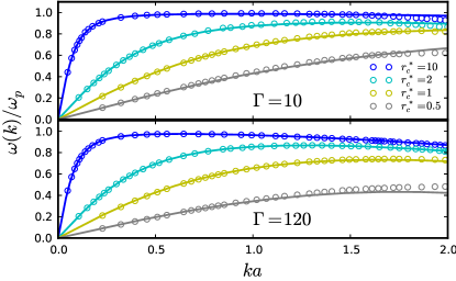
Figure 4: (color online) Brillouin peak position as obtained from MD (open circles), and the prediction of Eq. (2) (solid lines).

For finite $r_{c}^{*}$, the mean field only begins to play a role when $kr_{c}>0.43$, i.e. when the range of the potential is large compared to the lengthscale of the density variations. Therefore one may expect that for $r_{c}^{*}=\infty$, when the interaction potential is Coulombic OCPnote , the mean field is important at all lengthscales (in this case, our criterion $k_{max}r_{c}\simeq 0.43$ gives $k_{max}=0$ !). To be sure, the peculiarity of the Coulomb potential is very well known - in this case the longitudinal waves are not low frequency sound waves as for $r_{c}^{*}<\infty$ but instead high frequency plasma waves ($\omega\approx\omega_{p}$), even at $k=0$. The resulting ‘plasmon’ peak in $S(k,\omega)$, the position of which is illustrated in Fig. 2 (red triangles), is certainly not described by the low-frequency hydrodynamic equations that lead to Eq. (Applicability of the hydrodynamic description of classical fluids) - one can indeed wonder why hydrodynamics should describe plasma oscillations at all. The difficulty here is underlined by a kinetic theoretical derivation of the hydrodynamic equations BausHansen : when proceeding with the Chapman-Enskog expansion of the appropriate kinetic equation, the mean field term is usually treated as a small perturbation since in the small-gradient region of interest to hydrodynamics the kinetic equation is always dominated by the collision term. In this case, however, the mean field term cannot be considered as small since its straightforward small-gradient expansion diverges with the characteristic Coulomb divergence (see BausHansen and references therein). Based on this analysis, Baus and Hansen BausHansen argued that only when the collisionality dominates the mean field, which they predicted would occur at sufficiently high coupling strength $\Gamma$, could a hydrodynamic description be expected. In this case the hydrodynamic description is identical to Eq. (Applicability of the hydrodynamic description of classical fluids) gammanote but with $c_{s}k$ replaced with $\omega_{p}(1+\frac{c_{s}^{2}k^{2}}{2\omega_{p}^{2}})$ Vieillefosse . This macroscopic description is known not to work for small $\Gamma$ BausHansen ; exactly how large $\Gamma$ has to be for it to be applicable was left as an open question until now. We show here that in fact the hydrodynamic description is not valid at any $\Gamma$.

Baus and Hansen BausHansen based the arguments outlined above on an exact formula for $S(k,\omega)$, derived using generalised kinetic theory , which at small $k$ is given by gammanote

$$\frac{S^{B}(k,\omega)}{S(k)} = \frac{bk^{2}}{(\omega+\omega_{p}(1+\frac{k^{2}}{2}a))^{2}+(\frac{k^{2}}{2}b)^{2}}$$ (3)

$$+ \frac{bk^{2}}{(\omega-\omega_{p}(1+\frac{k^{2}}{2}a))^{2}+(\frac{k^{2}}{2}b)^{2}}\,,$$

where $a$ and $b$ are generalised coefficients with $k$ and $\omega$ dependence. They were able to show that only at large $\Gamma$ would it be possible for these coefficients to equal their macroscopic counterparts (of Eq. (Applicability of the hydrodynamic description of classical fluids)), $c_{s}^{2}/\omega_{p}^{2}$ and $2\sigma$ respectively BausHansen . We have estimated $a$ and $b$ by fitting $S(k,\omega)$ at the smallest $k$ value accessible to our MD simulations to Eq. (3) - this gives a very good fit. However, as shown in Table 1, the values obtained for $a$ and $b$ do not agree at all with their macroscopic counterparts, even at our highest coupling strength of $\Gamma=175$, which is close to the freezing point of the system BausHansen . For example, the width of the plasmon peak $b$ does not even follow the same trend predicted by the hydrodynamic scaling $2\sigma$ at our higher $\Gamma$ values. From this we conclude that the combination of mean field and collisional effects means that the hydrodynamic description à la Navier Stokes is not valid for a Coulomb system at any coupling strength $\Gamma$.

$\Gamma$	$a$	$c_{s}^{2}/\omega_{p}^{2}$	$b$	$2\sigma$
1	0.895	0.304	0.192	1.825
5	0.088	-0.034	0.109	0.333
10	-0.009	-0.080	0.078	0.235
50	-0.056	-0.112	0.032	0.212
120	-0.062	-0.127	0.021	0.349
175	-0.065	-0.129	0.009	0.550

Table 1: Comparison of the generalised coefficients obtained by fitting the MD $S(k,\omega)$ at our smallest $k$ value to Eq. (3) with the analogous coefficients that appear in the hydrodynamic description. $c_{s}$ is determined from the internal energy fit given in DeWitt , while $\sigma$ is obtained from Daligault .

In summary, for finite range potentials, $r_{c}^{*}<\infty$ , we find that the hydrodynamic description is (i) always valid at sufficiently long lengthscales where ‘sufficiently long’ is determined by the range of the potential ($k_{max}r_{c}\simeq 0.43$) (ii) extremely accurate at these long lengthscales for all $\omega$ where $S(k,\omega)$ is not negligibly small (iii) not enlarged in its applicability as the level of many-body correlations in the system (i.e. $\Gamma$) is increased and (iv) is significantly extended in applicability by including a ‘mean field’ term in the macroscopic equations. For a Coulomb system, $r_{c}^{*}=\infty$, although the macroscopic approach correctly predicts the plasmon peak at $k=0$, for $k>0$ the persistence of both mean field and collisional effects causes the ordinary hydrodynamic approach to fail.

This work was supported by the John Fell Fund at the University of Oxford and by EPSRC grant no. EP/G007187/1. The work of J.D. was performed for the U.S. Department of Energy by Los Alamos National Laboratory under Contract No. DE-AC52-06NA25396.

References

- (1) L.D Landau and E.M. Lifshitz, Fluid Mechanics (Butterworth-Heinemann, 1987).
- (2) M.M. Mansour et. al., Phys. Rev. Lett. 58, 874 (1987).
- (3) T. Scopigno et. al., Phys. Rev. E 65, 031205 (2002).
- (4) M. Gedalin, Phys. Rev. Lett. 76, 3340 (1996).
- (5) I. Bouras et. al., Phys. Rev. Lett. 103, 032301 (2009).
- (6) M. Baus and J.P. Hansen, Phys. Rep. 59, 1 (1980), in particular section 4.4.
- (7) U. Balucani and M. Zoppi, Dynamics of the Liquid State (OUP, 2002).
- (8) S.H. Glenzer and R. Redmer, Rev. Mod. Phys. 81, 1625 (2009).
- (9) Z. Donkó, G.J. Kalman and P Hartmann, J. Phys.: Condens. Matter 20, 413101 (2008).
- (10) E. Garcia Saiz et. al., Nat. Phys. 4, 940 (2008); K. Wünsch et. al., Phys. Rev. E 79, 010201 (2009).
- (11) S. Ichimaru, Rev. Mod. Phys. 54, 1017 (1982).
- (12) J. Daligault, Phys. Rev. Lett. 96, 065003 (2006).
- (13) J.P. Hansen and I.R. McDonald, Theory of Simple Liquids (third edition) (Academic Press, 2006).
- (14) S.H. Glenzer et. al., Phys. Rev. Lett. 98, 065002 (2007).
- (15) R. Hockney and J. Eastwood, Computer Simulations Using Particles (McGraw-Hill, New York, 1981).
- (16) J.P. Mithen et. al., in preparation.
- (17) J.P. Boon and S. Yip, Molecular Hydrodynamics (Dover, 1980).
- (18) S. Hamaguchi, R.T. Farouki and D.H.E. Dublin, J. Chem. Phys. 105, 7641 (1996); T. Saigo and S. Hamaguchi, Phys. Plasmas 9, 1210 (2002); Z. Donko and P. Hartmann, Phys. Rev. E 69, 016405 (2004).
- (19) G. Salin, Phys. Plasmas 14, 082316 (2007).
- (20) We note also that for the Coulomb potential, the system is required to have a uniform (inert) neutralising background.
- (21) here we assume for simplicity; this does not affect our discussion and is also a good approximation.
- (22) P. Vieillefosee and J.P. Hansen, Phys. Rev. A 12, 1106 (1975).
- (23) H. DeWitt and W. Slattery, Contrib. Plasma Phys. 39, 97 (1999).