Dissipation Coefficients from Scalar and Fermion Quantum Field Interactions

Abstract

Dissipation coefficients are calculated in the adiabatic, near thermal equilibrium regime for a large class of renormalizable interaction configurations involving a two-stage mechanism, where a background scalar field is coupled to heavy intermediate scalar or fermion fields which in turn are coupled to light scalar or fermion radiation fields. These interactions are typical of warm inflation microscopic model building. Two perturbative regimes are shown where well defined approximations for the spectral functions apply. One regime is at high temperature, when the masses of both intermediate and radiation fields are less than the temperature scale and where the poles of the spectral functions dominate. The other regime is at low temperature, when the intermediate field masses are much bigger than the temperature and where the low energy and low three-momentum regime dominate the spectral functions. The dissipation coefficients in these two regimes are derived. However, due to resummation issues for the high temperature case, only phenomenological approximate estimates are provided for the dissipation in this regime. In the low temperature case, higher loop contributions are suppressed and so no resummation is necessary. In addition to inflationary cosmology, the application of our results to cosmological phase transitions is also discussed.

In Press JCAP (2011).

I Introduction

Many physical processes involving adiabatic dissipative effects near thermal equilibrium occur in relativistic systems of bosonic and fermionic quantum fields. In the evolution of the early universe, several phase transition are believed to have occurred, with Grand Unified, Electroweak, quantum cromodynamics (QCD), and chiral amongst the most commonly studied, and for both first and second order type transitions. Many physical implications are associated with these transitions including baryogenesis, defect formation, magnetic field formation, and relic particle production. In all such cases, interactions of the order parameter, typically a scalar field, with other fields will lead to various dissipative effects, and these effects, though not always accounted for, can have significant influence on physical processes.

An example of a phase transition in which dissipation has significant influence and even changes the basic dynamical nature of the process has been seen in the inflationary universe scenario. This scenario involves the evolution of a scalar field which during the process of changing phases of the system also induces inflationary expansion of the universe. In the standard picture of inflation ci , the inflaton field is modelled such that the interactions with other fields play no role during inflationary expansion. This leads to a thermodynamic supercooled phase in the universe during inflation. After this, to end inflation and put the universe back into a radiation dominated phase, the inflaton enters a period of coherent oscillations, where interactions with other fields now become important to reheat the universe with particles reheatu . An alternative to this cold inflation picture is to consider dynamics where the inflaton interacts with other fields all during inflation. In such a case, dissipative effects become important and the dynamics of inflation is completely altered. In this warm inflationary dynamics Berera:1995ie , radiation production occurs concurrent with inflationary expansion, and the seeds of density perturbation are thermal in origin im ; Berera:1995wh ; Berera:1999ws , thus significantly altering the observable signatures of inflation compared to cold inflation.

Our primary motivation for the dissipative coefficients calculated in this paper is for their application to warm inflationary cosmology. However, our results may also have a broader range of applications in different contexts involving the nonequilibrium dynamics of fields, and we will briefly discuss these possibilities later in the paper.

Typical warm inflation models involve a two-stage field interaction mechanism, where a scalar field is coupled to another intermediate field which in turn is coupled to yet another decay field. The intermediate field (which will be called the “catalyst” field) is a heavy field (in this paper we consider it either a scalar or a fermion) that can decay into light fields (which will be called “radiation” fields and will here again be either scalars and/or fermions). These types of interactions, although naturally emerge in the hierarchy of interactions, were first realized for calculations of dissipation coefficients from model building applications to warm inflation and the interaction structure was generically termed as the two-stage mechanism BR1 (for recent reviews, please see BMR ; BasteroGil:2009ec ). These two-stage interactions, although more complicated than the direct interactions, where the relevant field modes would directly decay in light radiation particles, offer some simplifying features. For one thing, in the regime where the intermediate field mass is heavy relative to the temperature whereas the radiation fields are light, what we term the low-temperature regime, we can show that leading order contributions suffice in general to give a reliable estimate for the dissipation coefficient. This may not be the case in the regime where both the intermediate and final field masses are small relative to the temperature, what we term the high-temperature regime, where a different coupling governs the vertex compared to the decay width and the appearance of infrared and near on-shell divergences preclude the need for resummation of higher order terms, as we will detail later on.

In this paper we compute dissipation coefficients coming from intermediate fields, either scalars or fermions, in two-stage field interacting models, in the adiabatic, near thermal equilibrium regime. Within this work, we develop a very new approximation which we call the low-momentum approximation. We show in this paper, both analytically and numerically that this low-momentum approximation is valid for the low-temperature regime, where a heavy mass field is involved in mitigating the interaction between the background field and the light fields. This low-momentum approximation was first applied in BMR ; mossxiong0 . In this paper we will further extend those earlier results and give a detailed analysis of the possible different temperature regimes that can be defined in terms of the different energy scales involved.

To contrast the analysis in this paper of this new low-momentum approximation, there is another very common approximation used in the literature, which picks out the poles of the propagators as dominating the integral expressions of dissipative coefficients. We will refer to this as the pole approximation. One key result we will show in this paper is for these sorts of two-stage processes where the scalar background field interacts with the light radiation fields via heavy catalyst fields, in the low-temperature regime, defined as where the heavy catalyst field masses are much bigger than the temperature scale, this new low-momentum approximation dominates over the pole approximation. In particular, if one extended the pole approximation down into this low-temperature regime, one would find exponentially damped behavior for the dissipative coefficients. However, since the low-momentum approximation dominates this effect, the result is that the dissipative coefficients damp much slower, as a power law with respect to temperature, and so are much bigger in the regime of low-temperature, as compared to the results that would be obtained from the pole approximation.

This paper focuses only on renormalizable two-stage interactions between scalar and fermion fields. A thorough analysis of dissipation coefficients for many of the applications stated above, also require treating gauge fields, which is beyond the scope of this paper, but we plan to examine them in a future paper. Nevertheless, even in gauge theories, there are interactions of the sorts computed in this paper, which up to now have not been treated in the literature.

The paper is organized as follows. In Sect. II we briefly review the physics and definitions leading to the appearance of dissipative terms in the effective equations of motion for background fields. In Sect. III we specify all the interaction Lagrangian densities which we will treat in the paper. Particular attention is given to the interactions relevant to the two-stage mechanism BR1 , where dissipative effects are determined by the decay of a heavy intermediate field into light fields, with the former coupled to a relevant background field, whose dynamics we are interested in. The formal expressions for calculation of the dissipative coefficients, within the model interactions and decay forms we considered in our derivations, are given in Sect. IV. In Sect. V we give a physical interpretation of the dissipation coefficients by showing their connection with particle production. In Sect. VI the spectral functions, which are the fundamental quantities needed for calculating the dissipation coefficients, are computed. The results for dissipation coefficients in the very low, low and high-temperature regimes are presented in Sect. VII. Various applications of these coefficients to inflation and phase transitions in general are examined in Sect. VIII. Section IX gives our summary and concluding remarks. Two Appendices are also included to give technical details. In Appendix A we show possible model building realizations of the type of interactions we consider in this paper. In Appendix B we give some of the details for the calculations of the imaginary parts of the relevant self-energy contributions considered in this paper and the corresponding particles decay widths.

II Dissipation Coefficients

In this section we describe how dissipation coefficients are defined in quantum field theory. We start by discussing the definition and derivation of the dissipation coefficient in a generic interacting quantum field theory model.

A system, displaced from a state of equilibrium, when interacting with an environment, is expected to exhibit non-unitary evolution. The system dynamics will typically experience dissipative effects as it returns to its equilibrium state. A common example involving quantum fields is the case of some background scalar field $\varphi$ that is interacting with other fields, with $\varphi$ having an amplitude that is initially displaced from equilibrium. Let us describe this field theory model as having standard kinetic terms and with a potential given by

$$V(\varphi,X)=V(\varphi)+V_{\rm int}(\varphi,X)\;,$$ (1)

where $X$ represent any other field or degree of freedom that is coupled to the background field and $V_{\rm int}(\varphi,X)$ gives how this background field is coupled to this other field. A proper study of the evolution of this background field can be performed in the context of the in-in, or the closed-time path (CTP) functional formalism (for an introduction, see for example bellac ). By integrating over the $X$ field, a nonlocal effective equation of motion for $\varphi$ can be derived. If we write the interaction term in Eq. (1) as

$$V_{\rm int}(\varphi,X)=f(\varphi)g(X)\;,$$ (2)

then an ensemble averaged effective equation of motion for the system, described by the background field $\varphi$, has the generic form up to first order in the nontrivial nonlocal terms (see also Ref. calzetta+hu for a recent review)

$$\partial_{\mu}\frac{\partial{\cal L}_{\rm eff,r}[\varphi]}{\partial(\partial_{\mu}\varphi)}-\frac{\partial{\cal L}_{\rm eff,r}[\varphi]}{\partial\varphi}-i\frac{\partial f(\varphi)}{\partial\varphi}\int d^{4}x^{\prime}\theta(t-t^{\prime})\left[f(\varphi(x^{\prime}))-f(\varphi(x))\right]\langle[g(X(x)),g(X(x^{\prime}))]\rangle=0\;,$$ (3)

where ${\cal L}_{\rm eff,r}[\varphi]$ is the renormalized effective Lagrangian density for $\varphi$ and $\langle\cdots\rangle$ are ensemble averages with respect to an equilibrium (quantum or thermal) state. These ensemble averages over the fields can also be conveniently expressed in terms of the causal two-point Green’s functions for the fields $X$, as shown e.g. in Refs. GR ; BGR ; BR1 ; BMR ; BR21 ; BR22 , with the form of the nonlocal term in Eq. (3) dependent on the form for the interaction term $V_{\rm int}(\varphi,X)$. A simple case is for example when we have a bi-quadratic interaction of the scalar field $\varphi$, assumed homogeneous, $\varphi\equiv\varphi(t)$, with some other scalar field represented by $X$,

$$V_{\rm int}(\varphi,X)=\frac{g_{1}^{2}}{2}\varphi^{2}X^{2}\;.$$ (4)

In this case, the nonlocal term in Eq. (3) becomes GR

$$-i\frac{\partial f(\varphi)}{\partial\varphi}\int d^{4}x^{\prime}\theta(t-t^{\prime})\left[f(\varphi(x^{\prime}))-f(\varphi(x))\right]\langle[g(X(x)),g(X(x^{\prime}))]\rangle$$

$$=2g_{1}^{4}\varphi(t)\int_{-\infty}^{t}dt^{\prime}\left[\varphi(t^{\prime})^{2}-\varphi(t)^{2}\right]\int\frac{d^{3}{\bf p}}{(2\pi)^{3}}{\rm Im}\left[G_{X}^{++}({\bf p},t,t^{\prime})\right]^{2}_{t>t^{\prime}}\;,$$ (5)

where $G_{X}^{++}({\bf p},t,t^{\prime})$ is the spatial Fourier transformed causal two-point propagator for the $X$ field.

The non-local term in the effective equation of motion represents a transfer of energy from the $\varphi$ field into radiation, i.e. it is a dissipative effect. Such terms can be localized when there is a separation of timescales in the system (for discussion about the validity of the localization approximation for the nonlocal term and region of parameters where this can be achieved in specific models, see e.g. Refs. BMRnoise ; BMR ). Suppose, for example, that the self-energy introduces a response timescale $\tau$. If $\varphi$ is slowly varying on the response timescale $\tau$,

$$\frac{\dot{\varphi}}{\varphi}\ll\tau^{-1},$$ (6)

which is typically referred to as the adiabatic approximation, then we can use a simple Taylor expansion and write

$$f(\varphi(t^{\prime}))-f(\varphi(t))=(t^{\prime}-t)\,\dot{\varphi}(t)\frac{\partial f(\varphi)}{\partial\varphi}+\dots$$ (7)

The effective equation of motion for $\varphi$ (assumed homogeneous) including the linear dissipative terms then becomes

$$\ddot{\varphi}+\Upsilon\dot{\varphi}+\frac{\partial V_{\rm eff.r}(\varphi)}{\partial\varphi}=0\;,$$ (8)

where $V_{\rm eff,r}(\varphi)$ is the renormalized effective potential and $\Upsilon$ is the dissipation coefficient defined as

$$\Upsilon=\int d^{4}x^{\prime}\,\Sigma_{R}(x,x^{\prime})\,(t^{\prime}-t),$$ (9)

where $\Sigma_{R}(x,x^{\prime})$ is a retarded correlation that depends on the specific form of the interaction $V_{\rm int}(\varphi,X)$ and is defined by

$$\Sigma_{R}(x,x^{\prime})=-i\left[\frac{\partial f(\varphi)}{\partial\varphi}\right]^{2}\theta(t-t^{\prime})\langle[g(X(x)),g(X(x^{\prime}))]\rangle\;.$$ (10)

III Interaction Terms

In this work we are interested in examining the case where a scalar field $\phi$ has a background value $\langle\phi\rangle=\varphi(t)$. This field could be, for example, the order parameter in some phase transition or the inflaton field during cosmic inflation. For the purposes of these calculations, the scalar field $\phi$ is treated generically. This field is coupled to other boson $\chi$ and fermion $\psi_{\chi}$ fields, which will be called the “catalyst fields”. These fields are in turn coupled to bosonic $\sigma$ and fermionic $\psi_{\sigma}$ fields, which will be called the “radiation fields”. We will compute the dissipation coefficients for the interaction structures listed below. The combination of all the interaction types to be considered encompass most of the couplings between scalars and fermions that emerge in particle physics models. In particular, they can be combined with appropriately chosen coupling constants to be applicable in Supersymmetric (SUSY) models, such as often used in cosmological warm inflation model building BasteroGil:2006vr ; BasteroGil:2009ec . Alternatively they can be used independently. In Appendix A we will give some examples.

Next we specify the different types of interactions we will consider. The interactions between catalyst and radiation fields are:

1. Interaction between the scalars $\chi$ and $\sigma$:

   $${\cal L}_{I}[\chi,\chi^{\dagger},\sigma,\sigma^{\dagger}]=-h_{1}M[\chi^{\dagger}\sigma^{2}+\chi(\sigma^{\dagger})^{2}]-g_{3}^{2}\chi^{\dagger}\chi\sigma^{\dagger}\sigma\;,$$ (11)

   where $h_{1}$ and $g_{3}$ are coupling constants and $M$ is a mass term (in SUSY models this often is $M=g_{1}\varphi/\sqrt{2}$, where $\varphi$ is the background inflaton field).

2. Yukawa interaction between the scalar $\chi$ and fermions $\psi_{\sigma}$, $\bar{\psi}_{\sigma}$:

   $${\cal L}_{I}[\chi,\chi^{\dagger},\psi_{\sigma},\bar{\psi}_{\sigma}]=-h_{2}[\chi^{\dagger}\bar{\psi}_{\sigma}P_{R}\psi_{\sigma}+\chi\bar{\psi}_{\sigma}P_{L}\psi_{\sigma}]\;,$$ (12)

   where $P_{R({L})}=(1\pm\gamma_{5})/2$ are the chiral projection operators.

3. Yukawa interaction between the scalar $\sigma$ and fermions $\psi_{\sigma},\bar{\psi}_{\sigma},\psi_{\chi},\bar{\psi}_{\chi}$:

   $${\cal L}_{I}[\sigma,\sigma^{\dagger},\psi_{\sigma},\bar{\psi}_{\sigma},\psi_{\chi},\bar{\psi}_{\chi}]=-h_{3}[\sigma^{\dagger}\bar{\psi}_{\chi}P_{R}\psi_{\sigma}+\sigma\bar{\psi}_{\sigma}P_{L}\psi_{\chi}]\;.$$ (13)

The interactions between the scalar $\phi$ field and the other fields are:

1. Interaction between the scalars $\phi$ and $\chi$:

   $${\cal L}_{I}[\phi,\phi^{\dagger},\chi,\chi^{\dagger}]=-g_{1}^{2}\phi^{\dagger}\phi\chi^{\dagger}\chi\;,$$ (14)

   where, without loss of generality, the background scalar field is associated with the zero mode of the real component of $\phi$: $\phi=(\phi_{1}+\varphi+i\phi_{2})/\sqrt{2}$. From Eq. (14), the relevant term that will contribute to dissipation in the scalar fields effective equation of motion, at one-loop order, is then $-g_{1}^{2}\varphi^{2}|\chi|^{2}/2$.

2. Interaction between the scalar $\phi$ and the fermions $\psi_{\chi}$, $\bar{\psi}_{\chi}$,

   $${\cal L}_{I}[\phi,\phi^{\dagger},\psi_{\chi},\bar{\psi}_{\chi}]=-g_{2}[\phi^{\dagger}\bar{\psi}_{\chi}P_{R}\psi_{\chi}+\phi\bar{\psi}_{\chi}P_{L}\psi_{\chi}]\;,$$ (15)

   where, in this case, the relevant term that will contribute to the scalar field’s effective equation of motion, is $-g_{2}(\varphi/\sqrt{2})\bar{\psi}_{\chi}\psi_{\chi}$.

3. Interaction among the three scalars $\phi$, $\chi$ and $\sigma$:

   $${\cal L}_{I}[\phi,\phi^{\dagger},\chi,\chi^{\dagger},\sigma,\sigma^{\dagger}]=-g_{1}h_{1}[\phi^{\dagger}\chi^{\dagger}\sigma^{2}+\phi\chi(\sigma^{\dagger})^{2}]\;.$$ (16)

   Note that the interaction (11) is the term dependent on the scalar background field, derived from (16) once $\phi$ is written in terms of $\varphi$ and $M$ is then associated with $g_{1}\varphi/\sqrt{2}$. The interaction term (16) only contributes to the dissipation in the scalar field’s effective equation of motion at two-loop order.

Finally there can be self-interactions for the scalars:

$${\cal L}_{I}[\phi,\phi^{\dagger}]+{\cal L}_{I}[\chi,\chi^{\dagger}]+{\cal L}_{I}[\sigma,\sigma^{\dagger}]=\lambda_{\phi}(\phi\phi^{\dagger})^{2}+\lambda_{\chi}(\chi\chi^{\dagger})^{2}+\lambda_{\sigma}(\sigma\sigma^{\dagger})^{2}\;.$$ (17)

In the interaction forms considered above, at tree-level $\phi$ is only coupled to either the scalar boson $\chi$ or fermion $\psi_{\chi}$. In the presence of a vacuum expectation value $\varphi$, these can become heavier than the scalar $\sigma$ and fermion $\psi_{\sigma}$, which in turn are only coupled at tree-level with the intermediate fields $\chi$ and $\psi_{\chi}$. At the level of model interactions we are considering, there are radiative (loop generated) terms that can couple $\phi$ to $\sigma$ and $\psi_{\sigma}$, which can make them also heavy fields. These radiative generated interactions can however be kept small with either suitable choice of coupling constants or by imposing a symmetry for the model interactions (like SUSY). These possibilities, together with physical examples, are discussed in Appendix A. In the following sections we will always assume that the radiation scalar $\sigma$ and fermion $\psi_{\sigma}$ fields are lighter than the intermediate scalar boson $\chi$ or fermion $\psi_{\chi}$ fields; it is left as a model building question what conditions are required to achieve these conditions, but aside from some comments in Appendix A, those issues are beyond the subject of this paper.

III.1 Model Parameters

The calculation will be done for different thermal regimes depending on the relation between temperature $T$ and the field masses $m_{\chi},m_{\psi_{\chi}},m_{\sigma},m_{\psi_{\sigma}}$, for the $\chi$, $\psi_{\chi}$, $\sigma$ and $\psi_{\sigma}$ fields respectively:

• Very low-temperature regime: $m_{\chi},m_{\psi_{\chi}},m_{\sigma},m_{\psi_{\sigma}}\gg T$.

• Low-temperature regime: $m_{\chi},m_{\psi_{\chi}}\gg T\gg m_{\sigma},m_{\psi_{\sigma}}$.

• High-temperature regime: $m_{\chi},m_{\psi_{\chi}},m_{\sigma},m_{\psi_{\sigma}}\ll T$.

The very low-temperature regime has all field excitations suppressed by Boltzmann exponential factors, and thus so are the dissipation coefficients. In the low-temperature regime the interactions produce the two-stage catalyst induced dissipation of BR1 . This mechanism leads to dissipation that are not damped by Boltzmann exponential factors, despite the fact the $\chi$ and $\psi_{\chi}$ fields are heavy with respect to $T$. For the dissipative coefficients, the interactions that give the leading $T$ dependent terms have been calculated in mossxiong0 , but here we also present interactions that give less dominant terms with respect to $T$.

Dissipation coefficients have already been computed for the self-interacting scalar field, in particular in the high-temperature regime hosoya1 ; Masa . In this case, for example in the computation of dissipation coefficients in the local approximation, it demands much more stringent restrictions on the model parameters BGR ; BR1 ; BMRnoise than dissipation coming from $\phi$ interacting with other fields. We will not be interested in the dissipation effects from $\phi$ self-interaction. As such we will assume the $\phi$ self-coupling $\lambda_{\phi}=0$, or we can equivalently assume that $\phi$ is only a classical background field which is coupled to the remaining fields (considered as the bath or environment which is coupled to the system background field).

Concerning the magnitude of the many interaction terms considered above, we will restrict to values such that the leading contributions to the vacuum polarization terms (from which the decay terms are extracted and, as we will see below, enter in the calculations of the Green’s functions) will come dominantly from one-loop processes, when the decaying field is a heavy field (e.g. either $\chi$ or $\psi_{\chi}$). For instance, we will keep the leading one-loop order vacuum polarization terms for the catalyst (intermediate) fields $\chi$ and $\psi_{\chi}$ coming from the radiation fields $\sigma$ and $\psi_{\sigma}$, and that leads to decay processes like $\chi\to\sigma+\sigma$, $\chi\to\psi_{\sigma}+\bar{\psi}_{\sigma}$, and $\psi_{\chi}\to\sigma+\bar{\psi}_{\sigma}$, with complex conjugate analogous process. Decay processes for the light boson and fermion fields can only happen through Landau damping and, therefore vanish at zero temperature when on-shell. Decays for the heavy fields involving two-loop terms, like Landau damping coming from the fields self-interactions or the bi-quadratic interaction will be considered subdominant with respect the one-loop order processes. For this to be valid, the coupling constants in the interactions (11), (12), (13) and (17) should satisfy

$$g_{3}^{2}\ll h_{1},h_{2}$$

$$\lambda_{\chi}\ll h_{1},h_{2}\,.$$ (18)

On the other hand, decay processes involving one light and one heavy field are suppressed compared to the two-loop process involving the $\sigma$ self-interaction term with coupling $\lambda_{\sigma}$. The only restriction we impose on the $\sigma$ self-interaction magnitude is it to be small compared with the couplings, which then implies in the constraint

$$\lambda_{\sigma}\ll g_{3}^{2},h_{2}^{2},h_{3}^{2}\;,$$ (19)

so that temperature corrections to the heavy fields tree-level masses are larger than the temperature correction for the $\sigma$. This way we can also keep the effective (temperature dependent) masses for $\chi$ and $\psi_{\chi}$ still larger than that for the $\sigma$ and $\psi_{\sigma}$ in the high-temperature regime.

In the low-temperature regime, the above generic perturbative constraints are sufficient for consistent calculations at one-loop order with respect to the intermediate fields. In the high-temperature regime, however, computation of the dissipation coefficients are known to have issues regarding resummation of higher loop terms jeon1 ; jeon ; arnold . We will return later on to the issue of resummation when computing the dissipation coefficients in the high-temperature regime. There we will present some additional constraints on the model parameters, in addition to (18), so as to make the calculation consistent in that regime.

IV Dissipation Coefficients from Scalar and Fermion Interactions

This section presents the specific dissipation coefficients emerging from the interaction terms given in Sect. III and that appear in the $\phi$-field background effective equation of motion.

As discussed in Sec. II, the effective dynamics for the background scalar field when expressed in a local form is described by a dissipative equation of motion of the form Eq. (8), with dissipation coefficient $\Upsilon$ expressed in general by Eqs. (9) and (10).

As mentioned before, we will assume throughout that $\phi$ contributes only through its classical background field value. Moreover, these calculations will also be done in the adiabatic approximation Eq. (6) as well as

$$\frac{\dot{T}}{T}\ll\tau^{-1}.$$ (20)

Thus, regarding the interaction terms of the intermediate (catalyst) fields $\chi$ and $\psi_{\chi}$ presented in Sect. III, we find that $\Sigma_{R}$, the retarded correlation entering in the definition of the dissipation coefficient $\Upsilon$, Eq. (9), becomes

$$\Sigma_{R}(x^{\prime})=-i\left(\frac{g_{1}^{2}}{2}\right)^{2}\varphi^{2}\sum_{i=1}^{2}\theta(t-t^{\prime})\langle[\chi_{i}^{2}(x^{\prime}),\chi_{i}^{2}(0)]\rangle-i\frac{g_{2}^{2}}{2}\theta(t-t^{\prime}){\rm tr}\left\{\langle[\bar{\psi}_{\chi}(x^{\prime})\psi_{\chi}(x^{\prime}),\bar{\psi}_{\chi}(0)\psi_{\chi}(0)]\rangle\right\}\;,$$ (21)

where the first term in the above expression comes from the interaction (14) and the second term from (15). The dissipation coefficient $\Upsilon$ as defined here is derived for a system near thermal equilibrium. As such, the averages in Eq. (21) are over a thermal equilibrium distribution. Equation (21) is represented diagrammatically by Fig. 1, where only the relevant contributions to the vacuum polarization (as discussed in the previous section), which enter in the computation of the field propagators, are shown.

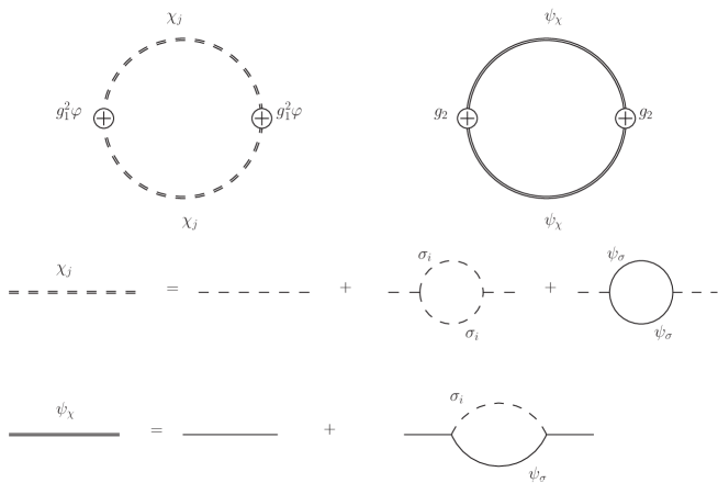
Figure 1: The contribution to the dissipation coefficient at leading order. The thick propagator lines are dressed scalar $\chi$ (dashed) or fermionic $\psi_{\chi}$ (solid) propagators (shown here including the relevant contributions to vacuum polarization at one-loop order).

In terms of the interactions given by Eqs. (14), (15) and (16), the dissipation coefficient at leading order is BMR ,

$$\Upsilon = \frac{2}{T}\left(\frac{g_{1}^{2}}{2}\right)^{2}\varphi^{2}\int\frac{d^{4}p}{(2\pi)^{4}}\left[\rho_{\chi_{1}}(p_{0},{\bf p})^{2}+\rho_{\chi_{2}}(p_{0},{\bf p})^{2}\right]n_{B}(p_{0})\left[1+n_{B}(p_{0})\right]$$ (22)

$$+ \frac{g_{2}^{2}}{2T}\int\frac{d^{4}p}{(2\pi)^{4}}{\rm tr}\left[\rho_{\psi_{\chi}}(p_{0},{\bf p})^{2}\right]n_{F}(p_{0})\left[1-n_{F}(p_{0})\right]\;,$$

where $\rho_{\chi}$ and $\rho_{\psi_{\chi}}$ are the spectral functions for the intermediate fields $\chi$ and $\psi_{\chi}$, defined in Sect. VI by Eqs. (26) and (28), and $n_{B}$ and $n_{F}$ are the Bose-Einstein ($n_{B}(\omega)=(e^{\beta\omega}-1)^{-1}$) and the Fermi-Dirac ($n_{F}(\omega)=(e^{\beta\omega}+1)^{-1}$) distributions, respectively, with $\beta\equiv 1/T$.

V Particle production interpretation

The physics involving the appearance of dissipation terms in the background effective equation of motion can be given an interpretation in terms of radiation (or particle) production. Such a physical interpretation for the dissipation term (9) has been given before BR21 ; BR22 ; BMR ; Graham . We here briefly review this interpretation in terms of the field interactions we are considering. Here dissipation can be seen as a result of energy being transferred from the $\phi$ field to the radiation bath fields $\sigma$ and $\psi_{\sigma}$ through the excitation of an intermediate field, which in this case are either the scalars $\chi$ or fermions $\psi_{\chi}$. That this is indeed associated to particle production ($\sigma$ and/or $\psi_{\sigma}$) has been demonstrated explicitly in Graham . In this case, the particle production rate for the radiation fields are only due to the interactions of $\chi,\psi_{\chi}$ with $\sigma,\psi_{\sigma}$, since the latter do not couple directly to the background field, except by the interaction term Eq. (16), which is however higher order (two-loop), in comparison to the other interactions. The particle production rate of the radiation bath particles due to interactions is Graham

$$\dot{n}={\rm Im}\left[2\int_{-\infty}^{t}dt^{\prime}\frac{e^{-i\omega({\bf p})(t-t^{\prime})}}{2\omega({\bf p})}\Sigma_{21}({\bf p},t,t^{\prime})\right]\;,$$ (23)

where $\omega({\bf p})$ is the particle dispersion relation for the scalars $\sigma$ or fermions $\psi_{\sigma}$ and $\Sigma_{21}=\Sigma_{\sigma,21}+\Sigma_{\psi_{\sigma},21}$ is the sum of the $\sigma$ and $\psi_{\sigma}$ self-energies (in the Schwinger-Keldshy formalism representation). $\dot{n}=\dot{n}_{\sigma}+\dot{n}_{\psi_{\sigma}}$ is the total particle production rate of the radiation bath particles $\sigma,\psi_{\sigma},\bar{\psi}_{\sigma}$ from the decay processes $\chi\to 2\sigma$, $\chi\to\bar{\psi}_{\sigma}+\psi_{\sigma}$ and $\psi_{\chi}\to\sigma+\bar{\psi}_{\sigma}$. The self-energies $\Sigma_{\sigma,21}$ and $\Sigma_{\psi_{\sigma},21}$ are obtained (or vice-versa) from the diagrams contributing to dissipation shown in Fig. 1, by cutting one of the internal loop (joining the external) lines for $\sigma$ (in the case of the $\sigma$ self-energy) or $\psi_{\sigma}$ (for the $\psi_{\sigma}$ self-energy). The diagrams representing these self-energies terms are shown in Fig. 2. An explicit expression for the self-energy is given for example in Graham .

Figure 2: Diagrams contributing to the self-energy of the radiation bath fields.

Using the expression of the total radiation energy,

$$\rho_{r}=\int\frac{d^{3}p}{(2\pi)^{3}}\omega({\bf p})n\;,$$ (24)

the dissipation coefficient Eq. (9) can be expressed as Graham

$$\Upsilon=\frac{\dot{\rho}_{r}}{\dot{\varphi}^{2}}=\frac{1}{\dot{\varphi}^{2}}\int\frac{d^{3}p}{(2\pi)^{3}}\left[\omega_{\sigma}({\bf p})\dot{n}_{\sigma}+\omega_{\psi_{\sigma}}({\bf p})\dot{n}_{\psi_{\sigma}}\right]\;.$$ (25)

This expression directly links the particle production of the bath radiation fields with how the background field dissipates its energy, represented by the dissipation coefficient $\Upsilon$.

VI Spectral Functions

Dissipation coefficients require the spectral functions for the scalar and the fermion fields. For the scalars (where $j=\chi_{1},\chi_{2},\sigma_{1},\sigma_{2}$ denote the real components of the complex scalar fields) we have:

$$\rho_{j}(p_{0},{\bf p}) = \frac{i}{-p_{0}^{2}+{\bf p}^{2}+m_{R,j}^{2}+i{\rm Im}\Sigma_{j}(p)}-\frac{i}{-p_{0}^{2}+{\bf p}^{2}+m_{R,j}^{2}-i{\rm Im}\Sigma_{j}(p)}$$ (26)

$$= \frac{4\omega_{j}({\bf p})\Gamma_{j}(p_{0},{\bf p})}{\left[-p_{0}^{2}+\omega_{j}({\bf p})^{2}\right]^{2}+\left[2\omega_{j}({\bf p})\Gamma_{j}(p_{0},{\bf p})\right]^{2}}\;,$$

where $\omega_{j}({\bf p})^{2}={\bf p}^{2}+m_{R,j}^{2}$, with $m_{R,j}$ the effective, renormalized mass for the scalar fields, $m_{R,j}^{2}=m_{j}^{2}+{\rm Re}\Sigma_{j}$. Also in Eq. (26) the decay width, $\Gamma_{j}(p_{0},{\bf p})$, is defined in terms of the imaginary part of the self-energy as

$$\Gamma_{j}(p_{0},{\bf p})=\frac{{\rm Im}\Sigma_{j}(p)}{2\omega_{j}({\bf p})}\;.$$ (27)

Note in the adiabatic approximation Eqs. (6) and (20), which underlies all calculations here for dissipation coefficients, the response time scale is typically associated with the decay widths, $\tau\rightarrow 1/\Gamma_{j}$.

For the fermions (where now $j=\psi_{\chi},\psi_{\sigma}$) we have that

$$\rho_{j}(p) = \frac{i}{\not\!p+m_{R,j}+i{\rm Im}\Sigma_{j}(p)}-\frac{i}{\not\!p+m_{R,j}-i{\rm Im}\Sigma_{j}(p)}\;,$$ (28)

where $m_{R,j}$ is the effective, renormalized mass for the fermion fields, $m_{R,j}=m_{j}+{\rm Re}\Sigma_{j}$. The imaginary part of the fermion self-energy appearing in Eq. (28) can be written, using rotational invariance, as (${\bf 1}$ is the 4x4 identity matrix)

$${\rm Im}\Sigma_{j}(p)=\gamma^{0}p_{0}\tilde{\alpha}_{0}+{\bf\gamma}.{\bf p}\tilde{\alpha}_{p}+m_{R,j}\tilde{\alpha}_{m}{\bf 1}\;,$$ (29)

where the expressions for $\tilde{\alpha}_{0},\tilde{\alpha}_{p}$ and $\tilde{\alpha}_{m}$ are explicitly given in Appendix B.

The imaginary part for the self-energies, appearing in Eqs. (26) and (28) are derived in Appendix B for completeness. The results for the decay widths are also given in Appendix B. For example, for the bosonic interaction Eq. (11), it is given by Eq. (68) with $g_{X}^{2}=4(h_{1}M/\sqrt{2})^{2}$, while for the Yukawa interaction Eq. (12), it is given by Eq. (71) with coupling factors now defined by $g_{X}^{2}=(h_{2}/\sqrt{2})^{2}$, and for the mixed boson-fermion interaction Eq. (13), it is obtained, likewise, from Eqs. (76) - (79), with $g_{X}^{2}=h_{3}^{2}$.

VII Dissipation Coefficients in the Low and High Temperature Regimes

An analysis of Eq. (22) indicates that the behavior of the dissipation coefficients in the different temperature and interaction regimes is determined by an interplay between the spectral function and the thermal occupation numbers. There are two regimes where well defined approximations can be made. One is the regime of fixed $T$ and where the couplings of the catalyst fields with the light fields, $h_{i}$, are going to zero. In this regime, the poles of the spectral functions will dominate the integral and this will be referred to as the pole approximation. The other regime is the integration region around low energy $p_{0}$ and low three-momentum ${\bf p}$, and this will be referred to as the low-momentum approximation. In the pole approximation, a well defined peak occurs in the spectral function, at an energy around the heavy particle dispersion relation. When the temperature is large, the occupation numbers are also large, and this approximation is valid. As such, the pole approximation works well in the high-$T$ region. In the low-momentum approximation, and at low temperatures, $T\leq m_{\chi},m_{\psi_{\chi}}$, the spectral function still has a well defined peak at around the heavy particle dispersion relation, but now this contribution is exponentially suppressed due to the occupation numbers in Eq. (22). However even at low $T$ the occupation numbers in the low energy and momentum region will not be exponentially suppressed, and so this approximation dominates over the pole contribution, which is hugely suppressed from the exponentially damped occupation numbers. Thus at low $T$ the low-momentum approximation dominates. Finally, at very low $T$ when also the decay widths become exponentially damped, both the pole and low-momentum approximation can be important, depending on the size of the couplings of the catalyst fields with the light fields, $h_{i}$, and the masses of all the particles involved.

Both approximations are now examined in detail. In the pole approximation, valid for fixed $T$ and $h\rightarrow 0$, the general expression for the dissipation coefficient Eq. (22) take on the simplified form,

$$\Upsilon \simeq \frac{1}{T}\left(\frac{g_{1}^{2}}{2}\right)^{2}\varphi^{2}\sum_{i=1}^{2}\int\frac{d^{3}p}{(2\pi)^{3}}\frac{1}{\Gamma_{\chi_{i}}(\omega_{\chi_{i}},{\bf p})\omega_{\chi_{i}}^{2}}n_{B}(\omega_{\chi_{i}})\left[1+n_{B}(\omega_{\chi_{i}})\right]$$ (30)

$$+ \frac{2g_{2}^{2}}{T}\int\frac{d^{3}p}{(2\pi)^{3}}\frac{m_{R,\psi_{\chi}}^{2}}{\Gamma_{\psi_{\chi}}(\omega_{\psi_{\chi}},{\bf p})\omega_{\psi_{\chi}}^{2}}n_{F}(\omega_{\psi_{\chi}})\left[1-n_{F}(\omega_{\psi_{\chi}})\right]\;,$$

where $\Gamma_{i}$ is the total decay width, e.g. for $\chi_{1,2}$ it is given by the sum of Eqs. (68) and (71), while for fermions, e.g. $\Gamma_{\psi_{\chi}}$, the fermion $\psi_{\chi}$ decay width is defined by the imaginary part of the pole of the fermion spectral function Eq. (28) and is given for example by Eq. (76).

For the low-momentum approximation, valid for fixed couplings $h_{i}$ and $T\rightarrow 0$, the spectral functions for the scalar boson fields becomes

$$\rho_{i}\simeq\frac{4}{m_{R,i}^{3}}\Gamma_{i}\;,$$ (31)

while the spectral function for the fermion fields, Eq. (28), becomes

$$\rho_{i}\simeq\frac{2}{m_{R,i}^{2}}\left(\tilde{\alpha}_{0}\gamma_{0}p_{0}+\tilde{\alpha}_{p}{\bf\gamma}.{\bf p}+m_{R,i}\tilde{\alpha}_{m}{\bf 1}\right)\;,$$ (32)

and then

$${\rm tr}(\rho_{i}^{2})\simeq 16\frac{(p_{0}^{2}\tilde{\alpha}_{0}^{2}-{\bf p}^{2}\tilde{\alpha}_{p}^{2}+m_{R,i}^{2}\tilde{\alpha}_{m}^{2})}{m_{R,i}^{4}}\;.$$ (33)

In this approximation, the dissipation coefficient, Eq. (22), using Eqs. (31) and (33), becomes

$$\Upsilon = \frac{2}{T}\left(\frac{g_{1}^{2}}{2}\right)^{2}\varphi^{2}\sum_{i}\int\frac{d^{4}p}{(2\pi)^{4}}\frac{16}{m_{R,i}^{6}}\Gamma_{i}^{2}\,n_{B}(p_{0})\left[1+n_{B}(p_{0})\right]$$ (34)

$$+ \frac{g_{2}^{2}}{2T}\int\frac{d^{4}p}{(2\pi)^{4}}16\frac{(p_{0}^{2}\tilde{\alpha}_{0}^{2}-{\bf p}^{2}\tilde{\alpha}_{p}^{2}+m_{R,i}^{2}\tilde{\alpha}_{m}^{2})}{m_{R,i}^{4}}n_{F}(p_{0})\left[1-n_{F}(p_{0})\right]\;.$$

Note from Eqs. (30) and (34) that the dependence of the dissipation coefficient on the heavy fields catalyst decay widths is very different in the two regimes where the pole and low temperature approximations are applicable. While in the pole approximation the dissipation coefficient is inversely proportional to $\Gamma_{i}$, in the low temperature regime it is proportional to $\Gamma_{i}^{2}$. These different dependencies will be of fundamental relevance when discussing higher order contributions to the dissipation as we will analyze later on. Next, we analyze the dissipation coefficient coming from the scalar and fermion interactions in the many different energy regimes with respect to the field masses and the temperature.

VII.1 Very Low Temperature Regime

In the very low-temperature regime, $T\ll m_{\sigma},m_{\psi_{\sigma}},m_{\chi_{i}},m_{\psi_{\chi}}$, the decay widths for the heavy fields into light fields, which can be read from Eqs. (68), (71) and (76), with $X$ the heavy field and the decay products $X_{1},X_{2}$ corresponding to the light fields, are dominated by the zero temperature contributions,

$$\Gamma_{\chi}^{(1)}\approx\left(\frac{h_{1}M}{\sqrt{2}}\right)^{2}\frac{1}{8\pi m_{\chi}}\;,$$

$$\Gamma_{\chi}^{(2)}\approx\left(\frac{h_{2}}{\sqrt{2}}\right)^{2}\,\frac{m_{\chi}}{8\pi}\;,$$

$$\Gamma_{\psi_{\chi}}\approx m_{\psi_{\chi}}\tilde{\alpha}_{m}\approx h_{3}^{2}\,\frac{m_{\psi_{\sigma}}}{4\pi}\;,$$ (35)

with temperature corrections that are Boltzmann suppressed by the heavy catalyst field masses.

Both the pole and low-momentum approximation have regions of validity and in both cases, as we will see below, the dissipation coefficient associated with a heavy field decay get exponentially suppressed. In general in this very low-temperature regime, for small couplings $h_{i}$, the pole approximation, Eq. (30) holds. The integrals in this expression are dominated by low three-momentum with respect to the field masses, to give

$$\Upsilon\stackrel{{\scriptstyle T\ll m,{\rm low}\;h}}{{\approx}}{\cal O}\left[\frac{g_{1}^{2}T^{2}}{\Gamma_{\chi}^{(1)}+T^{2}\Gamma_{\chi}^{(2)}/m_{\chi}^{2}}e^{-m_{\chi}/T}\right]+{\cal O}\left(\frac{g_{2}^{2}T^{2}}{\Gamma_{\psi_{\chi}}}e^{-m_{\psi_{\chi}}/T}\right).$$ (36)

For large values of couplings $h_{i}$ in this very low-temperature regime, the dominant contributions to the dissipation coefficient, Eq. (22), come from the low-momentum approximation to the spectral functions, Eqs. (31) and (32), with $p_{0},|{\bf p}|\ll m_{\chi_{i}},m_{\psi_{\chi}},m_{\sigma_{i}},m_{\psi_{\sigma}}$. Due to the Bose-Einstein and Fermi-Dirac distributions in Eq. (22), the larger contribution to the energy integrals now comes from $T\sim p_{0}$. The dissipation coefficient can then be approximated as

$$\Upsilon\stackrel{{\scriptstyle T\ll m}}{{\approx}}{\cal O}\left[\frac{g_{1}^{2}T^{3}}{m_{\chi}^{4}}\left(\Gamma_{\chi}^{(1)}+T^{2}\Gamma_{\chi}^{(2)}/m_{\chi}^{2}\right)^{2}\right]+{\cal O}\left(\frac{g_{2}^{2}T^{5}}{m_{\chi}^{4}}\Gamma_{\psi_{\chi}}^{2}\right)\;.$$ (37)

The behavior seen above is directly proportional to the square of the decay rates. If $p_{0}\gtrsim p$, the energy conditions in Eqs. (68), (71), (77), (79) and (78) cannot be satisfied and the the dissipation coefficient vanishes identically, $\Upsilon=0$. For $p_{0}\lesssim p$, only the Landau damping terms in the decay rates contribute. But these are exponentially (Boltzmann) suppressed, thus the dissipation coefficients in this case are negligibly small. As $T\to 0$, $\Upsilon\to 0$, as it is expected BMRnoise .

VII.2 Low Temperature Regime

The low-temperature regime is defined as $m_{R,\sigma},m_{R,\psi_{\sigma}}\ll T\ll m_{R,\chi_{i}},m_{R,\psi_{\chi}}$. In other words, this is the regime of low temperature with respect to the heavy catalyst fields but high temperature with respect to the radiation fields. In general the masses of the radiation bath fields $m_{\sigma},m_{\psi_{\sigma}}$ can be neglected. The temperature corrections to the effective masses of the heavy fields, due to the light field self-energies, can also be neglected, e.g., $m_{\rm R,\chi}^{2}\simeq m_{\chi}^{2}+(4\lambda_{\chi}+g_{3}^{2}+h_{2}^{2})T^{2}/12\approx m_{\chi}^{2}$ and $m_{\rm R,\psi_{\chi}}^{2}\simeq m_{\psi_{\chi}}^{2}+h_{3}^{2}T^{2}/12\approx m_{\psi_{\chi}}^{2}$, likewise for the light fermion field $\psi_{\sigma}$, whose loop radiative corrections, including the thermal ones, are suppressed by the heavy field masses, even though in this case the light fields are in the high-temperature regime. However the light scalar $\sigma$ field effective mass will get a temperature correction from self-interaction, $m_{R,\sigma}^{2}\simeq m_{\sigma}^{2}+\lambda_{\sigma}T^{2}/3$.

In this regime one can verify that the dominant contributions to the dissipation, Eq. (22), come from $p_{0},|{\bf p}|\ll m_{R,\chi_{i}},m_{R,\psi_{\chi_{i}}}$, which lead to the low-momentum approximation. There is also a regime for fixed $T$ and $h\rightarrow 0$ in which the pole approximation is valid. Since the temperature is small with respect the heavy field masses, the three momentum integration in Eq. (30) is dominated by $|{\bf p}|\ll m_{R,\chi_{i}},m_{R,\psi_{\chi_{i}}}$. In the pole approximation the decay widths are just given by the zero temperature results in Eqs. (68), (71) and (76). The behavior of the dissipation coefficient is, however, exponentially suppressed and of the form of Eq. (36).

For the case of fixed $h$ with $T\rightarrow 0$, the low-momentum approximation is valid, so the spectral functions can be approximated as Eqs. (31) and (32). The dissipation coefficient is now given by Eq. (34), which then leads in this low-temperature regime to the result:

$$\Upsilon \simeq \frac{g_{1}^{4}\varphi^{2}T^{3}}{8\pi^{5}}\sum_{i=1}^{2}\frac{1}{m_{R,\chi_{i}}^{6}}\left[A_{1}\frac{1}{m_{R,\chi_{i}}^{2}}\left(\frac{h_{1}M}{\sqrt{2}}\right)^{4}+B_{1}\left(\frac{h_{2}^{2}T^{2}}{m_{R,\chi_{i}}}\right)^{2}+2C_{1}\frac{h_{2}^{2}T^{2}}{m_{R,\chi_{i}}^{2}}\left(\frac{h_{1}M}{\sqrt{2}}\right)^{2}\right]+D_{1}\frac{g_{2}^{2}h_{3}^{4}}{64\pi^{5}}\frac{T^{5}}{m_{R,\psi_{\chi}}^{4}}\;,$$ (38)

where the constants in the above equation arise from evaluation of the momentum and energy integrals in Eq. (34). They have been evaluated numerically to give, $A_{1}\simeq 124.9$, $B_{1}\simeq 129.8$, $C_{1}\simeq 18.2$, $D_{1}\simeq 4362.6$.

Note from Eq. (38) that at leading order the dissipation coefficient goes as ${\cal O}(T^{3}/m_{\chi}^{2})$, agreeing with mossxiong0 . The dissipation coefficient obtained in this low temperature and low momentum regime is much less suppressed than what would be expected from the pole approximation case. In particular, we obtain no exponentially suppressed results as in the very low temperature regime.

The heavy fermion loop contribution is worth noting in Eq. (38). It is given by the last term on the RHS of that expression. The fermion contribution is sub-leading in the temperature in the low-$T$ regime, as compared with the term coming from the decay into only bosons.

This result can be explicitly verified by numerically solving the full expression, Eq. (22), and comparing with the respective approximations in each temperature regime case. This is done in Figs. 3 and 4, for choice of coupling $h=0.5$ (where we take for simplicity $h_{1}=h_{2}=h_{3}=h$ in the expressions for the decay widths) as function of temperature $T$, at both low and high temperature respectively. It is clear from Fig. 3 that as $T\ll m_{\chi}$, the low-momentum approximation agrees well with the full expression Eq. (22), whereas the pole expression agrees poorly as expected. The reliability of the results at high temperature, where the pole approximation is applicable, will be analyzed in more details in the next subsection.

From these comparisons, we see in all cases, the low-momentum approximation works well at very low temperatures $T/m_{\chi}\stackrel{{\scriptstyle<}}{{\sim}}0.04$, whereas at higher temperatures $T/m_{\chi}>1.0$, the pole approximation works well. The breakdown of the low-momentum approximation as $T$ increases arises because the occupation numbers in Eq. (22) no longer become exponentially suppressed, and so the contribution from the poles start to dominate. Results for the dissipation coefficient, coming from the individual interaction types, in the low-temperature regime, are summarized in Table 1.

${\cal L}_{I}$	dissipation $\Upsilon$
$-g_{1}^{2}\phi^{\dagger}\phi\chi^{\dagger}\chi-h_{1}M[\chi^{\dagger}\sigma^{2}+\chi(\sigma^{\dagger})^{2}]$	$0.026g_{1}^{4}h_{1}^{4}\varphi^{2}{T^{3}M^{4}}/{m_{R,\chi}^{8}}$
$-g_{1}^{2}\phi^{\dagger}\phi\chi^{\dagger}\chi-h_{2}[\chi^{\dagger}{\bar{\psi}}_{\sigma}P_{R}\psi_{\sigma}+\chi{\bar{\psi}}_{\sigma}P_{L}\psi_{\sigma}]$	$0.11g_{1}^{4}h_{2}^{4}\varphi^{2}{T^{7}}/{m_{R,\chi}^{8}}$
$-g_{1}^{2}\phi^{\dagger}\phi\chi^{\dagger}\chi-h_{1}M[\chi^{\dagger}\sigma^{2}+\chi(\sigma^{\dagger})^{2}]$	$0.015g_{1}^{4}h_{1}^{2}h_{2}^{2}\varphi^{2}{T^{5}M^{2}}/{m_{R,\chi}^{8}}$
$-h_{2}[\chi^{\dagger}{\bar{\psi}}_{\sigma}P_{R}\psi_{\sigma}+\chi{\bar{\psi}}_{\sigma}P_{L}\psi_{\sigma}]$
$-\frac{1}{\sqrt{2}}g_{2}\varphi{\bar{\psi}}_{\chi}\psi_{\chi}-h_{3}[\sigma^{\dagger}{\bar{\psi}}_{\chi}P_{R}\psi_{\sigma}+\sigma{\bar{\psi}}_{\chi}P_{L}\psi_{\sigma}]$	$0.22g_{2}^{2}h_{3}^{4}T^{5}/m_{R,\psi_{\chi}}^{4}$

Table 1: A summary of all the dissipation coefficients in the low-temperature regime coming from each of the interaction cases involving a heavy intermediate field (all expressions evaluated with $m_{\chi_{1}}=m_{\chi_{2}}$).

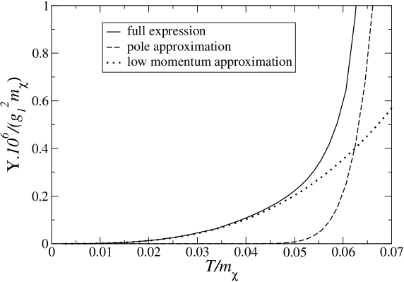
Figure 3: The behavior of the dissipation coefficient as a function of the temperature (in the low-temperature regime), for $g_{1}=g_{2}$, $h=h_{1}=h_{2}=h_{3}=0.5$, $m_{\sigma}=0.001m_{\chi}$ and $m_{\psi_{\chi}}=m_{\chi}$, $m_{\psi_{\sigma}}=m_{\sigma}$.

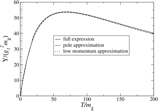
Figure 4: The behavior of the dissipation coefficient as a function of the temperature, for $g_{1}=g_{2}$, $h=h_{1}=h_{2}=h_{3}=0.5$, $g_{3}=0.01$, $m_{\sigma}=0.001m_{\chi}$ and $m_{\psi_{\chi}}=m_{\chi}$, $m_{\psi_{\sigma}}=m_{\sigma}$.

VII.3 High Temperature Regime

In this regime, we still have $m_{\sigma},m_{\psi_{\sigma}}\ll T$. As for the heavy catalyst field contributions, their effective thermal masses are $m_{\rm R,\chi_{i}}^{2}\simeq m_{\chi_{i}}^{2}+(4\lambda_{\chi}+g_{3}^{2}+h_{2}^{2})T^{2}/12$ and $m_{\rm R,\psi_{\chi}}^{2}\simeq m_{\psi_{\chi}}^{2}+h_{3}^{2}T^{2}/12$. Two temperature regions can be useful to define, $m_{\chi_{i}},m_{\psi_{\chi}}\ll T<\sqrt{12}m_{\chi_{i}}/\sqrt{4\lambda_{\chi}+g_{3}^{2}+h_{2}^{2}},\sqrt{12}m_{\psi_{\chi}}/h_{3}$, and $\sqrt{12}m_{\chi_{i}}/\sqrt{g_{3}^{2}+h_{2}^{2}},\sqrt{12}m_{\psi_{\chi}}/h_{3}<T$. In both cases Eq. (22) lead to a high-temperature expression for dissipative coefficient, which is dominated by the pole approximation and lead to the approximate expression Eq. (30). In this temperature regime, leading order one-loop expressions for these coefficients can become problematic as we will see below and are only valid in a restricted region of parameter space. The reason for this can be seen from how the dissipative coefficient in Eq. (30) depends on the field decay widths $\Gamma_{i}$. Since it is inversely proportional to $\Gamma_{i}$ and since the $\Gamma_{i}$ are proportional to the square of the coupling constants (see the results in Appendix B), loop corrections come with a ratio of the vertex coupling squared to the decay width coupling squared. Depending of the magnitude of these two couplings, in some parameter regimes higher loop correction terms to the dissipation will be the same order as the one-loop term, thus requiring resummation, and in other parameter regimes higher loop contributions will be suppressed.

VII.3.1 Resummation issues

It is worth recalling at this point the origin of this dependence on the couplings. At high temperature, diagrams contributing to the dissipation would have near on-shell singularities if only products of bare propagators were used. These singularities are softened by introducing explicit lifetimes for excitations, thus the decay widths $\Gamma_{i}$, through dressed propagators. This procedure leads to the result shown in Eq. (30) with a similar procedure at higher loops. The presence of these regulating thermal widths in the denominator then imply entire classes of diagrams, called ladder diagrams, which are diagrams with insertions of loops between the external propagators and in the definition of the dissipation they can contribute at the same order. This is much like what happens in the definition of viscosity coefficients from Kubo formulas as seen for example in Refs. jeon ; jeon1 , in the case of a single scalar field, and full resummation schemes to account for all the corrections occurring at the same order were used. Here we apply the outcome of this analysis for our case of field interactions involving light radiation and heavier catalyst fields.

Two possible examples of topologies of diagrams that can contribute beyond one-loop order are shown in Fig. 5. Higher order diagrams can be made with different variations of these topologies and similar ones.

Figure 5: Examples of topologies of diagrams that can contribute to the dissipation beyond the one-loop order.

Using the simple cutting rules explained e.g. in Refs. jeon ; jeon1 , let us first consider the contributions in the first topology shown by the top diagram in Fig. 5, which are the types of topologies contributing to dissipation due to the heavy catalyst scalar field $\chi$. Higher order contributions involve adding rungs to the simple leading order contribution, which are of the form of the rungs (a)-(e). The analysis from these contributions to dissipation shows propagators which can share pinching pole singularities. These are propagators for the fields running on the external part of the diagram that can share the same momentum when going on-shell, thus displaying near on-shell pinching poles. As mentioned above, these singularities are regulated by the field’s decay width, giving as a leading order contribution to the dissipation for instance a contribution of order $(g_{i}^{2}/\Gamma_{i})^{n}$, depending the type and number of rungs added to the diagram. For example, take for instance the case of a rung of type (a) shown in the top topology in Fig. 5. In this case the contribution of the rung (a) produces a multiplicative contribution to the leading order one-loop dissipation term that is ${\cal O}(\lambda_{\chi}^{2}/\Gamma_{\chi})$. $\Gamma_{\chi}$ receives contributions coming from the $\chi$ self-coupling vertex, $\sim{\cal O}(\lambda_{\chi}^{2})$, from the coupling with the light $\sigma$ bosons, $\sim{\cal O}(h_{1}^{2})$, and from light $\psi_{\sigma}$ fermions, $\sim{\cal O}(h_{2}^{2})$. In this case, this contribution can be rendered small compared to the one-loop result for the heavy field provided that $h_{1},h_{2}\gg\lambda_{\chi}$. Another possible contribution comes from rungs of type (b). Its contribution is ${\cal O}(g_{3}^{4}/\Gamma_{\chi})$, which can be rendered small by the same considerations taken for type (a). The next case are contributions involving rungs like type (c). Its contribution is now of ${\cal O}(g_{3}^{4}/\Gamma_{\sigma})$ The thermal width for $\sigma$ comes from the imaginary part of the self-energy terms for $\sigma$ built with the interactions (11), (13), (16) and its self-interaction term in (17). The leading order contributions from these interactions give $\Gamma_{\sigma}\sim{\cal O}(\lambda_{\sigma}^{2})+{\cal O}(h_{1}^{2})+{\cal O}(h_{3}^{2})+{\cal O}(g_{3}^{4})\sim{\cal O}(h_{1}^{2},h_{3}^{2})$. These contributions can also be rendered small, compared with the one-loop contribution with external propagators given by the heavy field $\chi$, with a suitable choice of couplings, e.g. $g_{3}\ll h_{1},h_{2},h_{3}$. The next two cases of contributions involves rungs of the form (d) and (e). The contributions of the form (d) gives ${\cal O}(h_{2}^{4}/(\Gamma_{\chi}\Gamma_{\psi_{\sigma}}))$. Since $\Gamma_{\psi_{\sigma}}\sim{\cal O}(h_{2}^{2}+h_{3}^{2})$ and using e.g. the typical parameters found in SUSY models displaying the types of interactions we have, the couplings will satisfy Eq. (52), and we find that these contributions can potentially be of ${\cal O}(1)$. Likewise, the contribution of type (e) for the couplings shown in Eq. (52) gives a parametric result of ${\cal O}(g^{4}/h^{2})$, which is higher order. The last topologies to be analyzed are the ones contributing to the dissipation coming from heavy catalyst fermion field and given by diagrams of the form of the bottom diagram shown in Fig. 5. The relevant additional rungs that appear are of the form of the terms (f) and (g) shown in that diagram. The contribution from rungs of the form (f) are parametrically ${\cal O}(h_{3}^{4}/(\Gamma_{\psi_{\chi}}\Gamma_{\psi_{\sigma}}))$. Using that $\Gamma_{\psi_{\chi}}\sim{\cal O}(h_{3}^{2})$, and parameters shown in Eq. (52), we find that this contribution is potentially of ${\cal O}(1)$. The other contribution comes from rungs of the form (g), which gives ${\cal O}(h_{3}^{4}/(\Gamma_{\psi_{\chi}}\Gamma_{\sigma}))\sim{\cal O}(1)$ using again Eq. (52). This contribution is also potentially of same order as the one-loop result for the dissipation due to heavy fermions in the higher temperature regime. The fermion dissipation, however, tend to be numerically smaller than the scalar field contributions to dissipation at high temperatures, as we will see from the results to be shown below and from those in Fig. 6.

VII.3.2 One-loop results

Though in principle all higher loop contributions to the dissipation can be re-summed using a variety of techniques, we will not attempt to do this here. The interactions considered in this paper are much more complex than the simple case of only a single scalar field, which was considered in previous works performing these resummations, and it would require a separate and thorough analysis to examine the necessary resummation. In any event, it is important to recognize that in contrast to the original analysis made e.g. in Refs. jeon1 ; jeon that had only a single coupling parameter, in our case where we have multiple coupling parameters and, as discussed above, we now have the added freedom to choose certain parameter regimes where some of higher loop contributions can be suppressed and no resummation for them are in principle necessary. This is true for example when computing particular contributions of fields, where for example, for those classes of diagrams that involve intermediate heavy field propagators and exemplified in the previous subsection. The cases that need special attention with respect to resummation are those where light field components run in the external part of the diagrams contributing to dissipation. This is e.g. the cases involving the inclusion of rungs of type (c) and (e) in the top topology shown in Fig. 5, or the rungs (f) and (g) in the second topology of the same figure, and seen in the parametric analysis performed previously.

Below we show some results for the dissipation at one-loop order at high temperatures, but these results are only meant to be phenomenological ones, providing an estimate for the dissipation, since they do not account for all the possible higher order loop contributions that they may receive.

In Fig. 4 are shown the result for the total dissipation coefficient, for the case of summing all the contributions, for temperatures up to two hundred times the intermediate field mass. Note that the low-momentum approximation quickly overestimates the true result as the temperature increases. The pole approximation becomes very good already at $T\sim m_{\chi},m_{\psi_{\chi}}$, but tends to slightly lose accuracy at higher temperatures, where the simple pole approximation, given in terms of the particles dispersion relation, becomes less accurate. This is more critical in the case when only decay into bosons are considered (e.g. with decay width given by Eq. (68)), and the temperature is such that $\Gamma_{\chi}^{(1)}/m_{\chi}\gtrsim 1$ (note that this cannot happen in the case of decay into fermions, where for large temperatures the decay width tends to zero (on-shell) due to Pauli blocking boya1 ).

It is also worth showing the individual contributions to the dissipation coming from the different intermediate catalyst fields and the different decay channels available to them. This is shown in Fig. 6.

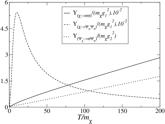
Figure 6: Individual contributions to the dissipation coefficient as a function of the temperature, for $g_{1}=g_{2}$, $h=h_{1}=h_{2}=h_{3}=0.5$, $g_{3}=0.01$, $m_{\sigma}=0.001m_{\chi}$ and $m_{\psi_{\chi}}=m_{\chi}$, $m_{\psi_{\sigma}}=m_{\sigma}$.

Note from Fig. 6 that for the cases of interaction of a scalar intermediate field with light scalars and interaction of an intermediate fermion with light scalar and fermion, the high temperature behavior is linear in temperature. Also, the dissipation from the interaction of an intermediate scalar field with light fermions dominates in the regime of temperature where $m_{\chi}\ll T\lesssim m_{\chi}/h_{2}$, but for $T\gg m_{\chi}/h_{2}$, the interaction of a intermediate scalar with light scalars dominates. For $T\gg m_{\chi}/h_{2}$ the contribution to dissipation coming from the interaction of an intermediate scalar field with light fermions tend quickly to become subdominant with respect to both the interaction of the intermediate heavy scalar $\chi$ with the light scalars $\sigma$ and the intermediate heavy fermion with the light scalars and fermions.

Approximate semi-analytical fitting formulas for the dissipation, valid in both high-temperature regimes, with respect to the masses of the intermediate fields, $m\ll T\lesssim m/h$ and $T\gg m/h$, and expressed in terms of the thermal masses for the intermediate scalar and fermion fields, can be obtained by considering separately the different interaction forms. Again, we cautioned that these results at high temperature are only meant to be interpreted phenomenologically, sincethey are only derived at leading one-loop order. The different cases are listed below (for simplicity all expressions below were evaluated with $m_{\chi_{1}}=m_{\chi_{2}}$):

a) Interaction of a heavy scalar into light scalar bosons, Eq. (11):

$$\Upsilon\approx 0.21\frac{g_{1}^{2}}{h_{1}^{2}}T\left\{1+3\left[\frac{m_{\chi}(T)}{T}\right]^{1/4}\right\}\;,$$ (39)

where the thermal mass $m_{\chi}(T)$ is here defined as $m_{\chi}^{2}(T)\simeq m_{\chi}^{2}+g_{3}^{2}T^{2}/12$, due to the interactions shown in Eq. (11).

b) Interaction of a heavy scalar into light fermions, Eq. (12):

$$\Upsilon\approx 7.3\frac{g_{1}^{2}}{h_{2}^{2}m_{\chi}}T^{2}\left[\frac{m_{\chi}}{m_{\chi}(T)}\right]^{3}\;,$$ (40)

where the thermal mass $m_{\chi}(T)$ is here defined as $m_{\chi}^{2}(T)\simeq m_{\chi}^{2}+h_{2}^{2}T^{2}/12$, due to the interactions shown in Eq. (12).

c) Interaction of a heavy fermion into a light scalar boson and light fermion, Eq. (13):

$$\Upsilon\approx 5.53\times 10^{-5}\frac{g_{2}^{2}T}{h_{3}^{2}}\left\{1+985.6\left[\frac{m_{\psi_{\chi}}(T)}{T}\right]^{14/9}\right\}\;,$$ (41)

where the thermal mass $m_{\psi_{\chi}}(T)$ is here defined as $m_{\psi_{\chi}}^{2}(T)\simeq m_{\psi_{\chi}}^{2}+h_{3}^{2}T^{2}/12$, due to the interactions shown in Eq. (13).

As noted above from the results of Fig. 6, the case of interaction of the intermediate scalar field $\chi$ with boson radiation fields $\sigma$ leads to growth linear in temperature of the dissipation coefficient at high temperature. This differs from the case of the scalar $\chi$ self-interacting, which found $1/T$ behavior hosoya1 ; GR ; BGR . The reason is, for the self-interacting case, the decay width at lowest order was at two-loops, whereas for the above case involving a separate radiation field, the decay width at lowest order is at one-loop. At one-loop the decay width is proportional to an imaginary part of the self-energy that is ${\cal O}(h_{1}^{2}m_{\chi}^{2})$, while at too-loop order, there are contributions GR ; BGR of ${\cal O}(g_{3}^{4}T^{2})$, coming from the interaction $g_{3}^{2}\chi^{2}\sigma^{2}$ and ${\cal O}(\lambda_{\chi}^{2}T^{2})$, coming from the $\chi$ field self-interaction, $\lambda_{\chi}\chi^{4}$. This difference in the decay rates at one-loop order and two-loops, results in the differing temperature behaviors observed for the dissipation. This difference in the leading behavior of the decay rates at one-loop and two-loop orders also imply that the one-loop contributions are dominant provided the temperature is not too high, that is, $T<{\rm min}(h_{1}m_{\chi}/g_{3}^{2},h_{1}m_{\chi}/\lambda_{\chi})$, which gives an additional constraint for the consistency of the derivations done here based on the contributions of one-loop polarizations only.

A crosscheck that the above estimates are at least parametrically correct even in the absence of a full resummation treatment can be made by noting the close relation between the general dissipation coefficient expression, Eqs. (9), (10), with those of the viscosity coefficients derived through the Kubo formulas jeon ; jeon1 . One observes that aside for differences in powers of momentum in the defining integrals, the expressions are similar. This similarity can be used to relate the dissipation coefficient with the known results for the viscosities, whose results, found for example in Refs. jeon ; jeon1 , account for the full resummation of ladder diagrams, just like the ones also contributing to the dissipation coefficient at high temperatures. This type of approach was used for instance by the author in Ref. Bodeker:2006ij to relate the moduli decay rate to the bulk viscosity coefficient. This was possible because of the interaction form used, which involved a derivative. This allowed turning the calculation of the dissipation coefficient in that reference to the analogous computation of the bulk viscosity through use of the Kubo formula. In our case, following the lead of Ref. Bodeker:2006ij , the proper analogy would be instead to relate our expressions for the dissipation with that for the shear viscosity (and properly accounting for the difference in powers of momentum in the integrals). This analogy was in fact raised before in Ref. BGR . In the simplest case of the interactions of the catalyst scalar field $\chi$ with only the radiation scalar field $\sigma$, this allow us to obtain an estimate for the shear viscosity as $\zeta_{\rm shear}\sim T^{5}/(h_{1}^{2}m_{\chi}^{2})$. The different temperature dependence with respect to the standard scalar field result obtained in the $\lambda\phi^{4}$ theory jeon , $\zeta_{\rm shear}\sim T^{3}/\lambda^{2}$, comes from the different contribution to the decay width $\Gamma$ in each case (as we noted in the previous paragraph, in the $\lambda\phi^{4}$ model $\Gamma$ comes from the imaginary part of the two-loop self-energy term, which is $\sim\lambda^{2}T^{2}$, while for the scalar catalyst-radiation interaction we consider here, it is dominated by the one-loop self-energy computed in the Appendix B). Relating the shear viscosity expression with our expression for the dissipation coefficient in this case (and accounting for the differences in factors of coupling constants and powers of temperature), in the high temperature regime we obtain $\Upsilon\sim g_{1}^{2}T/h_{1}^{2}$. This is parametrically the result we found in Eq. (39). Similarly, we could also relate the dissipation coefficient obtained for the other interaction forms. But this is still only meant to provide a parametric estimate for the dissipation coefficients, since they are not the complete resummation of all contributing higher order terms. Thus, we refrain ourselves from following any further this similarity between dissipation and viscosity coefficients in our case here, because it would also require a full calculation of the viscosity coefficients as well, which is beyond the scope of the present paper.

VII.3.3 Contrasting the derivation of the high versus low temperature dissipation coefficients

At this stage it is useful to contrast the derivation of the dissipation coefficients at high temperatures from this subsection with those obtained in the low temperature regime of subsection VII.2. One recalls from the calculations done in the previous subsection VII.2, that in the low-temperature case, where what we called the low-momentum approximation is valid, the dissipation coefficients are proportional to the square of the decay widths. This is evident from the behavior of the spectral functions, such as in Eqs. (31), (32) and from the explicit expression for the dissipation coefficient in that regime, Eq. (34). This very different behavior of the dissipation coefficients in the low-temperature regime is why they do not suffer from the problems seen for the high temperature regime. Due to this fact, it also means no resummation is required in the low-temperature case. Figure 3 provided one numerical example of parameter and low-temperature regimes where this low-momentum approximation is realized. As no resummation is needed, the one-loop expression for the dissipation coefficients in this regime alone provides reliable results.

It is also instructive and easy to understand the low-temperature dissipation coefficients by looking at the diagrams shown in Fig. 5. The dissipation coefficients always carry catalyst propagators in their upmost extreme points. Any higher order contribution to the dissipation coefficient would then have at least four external heavy catalyst field propagators. In this regime, the catalyst fields are at low-temperature, but the light radiation fields are at high temperatures. Thus, the rungs made with the light fields will be the ones that will have the most infrared sensitivity and that can produce ${\cal O}(1)$ contributions as seen from the analysis made following Fig. 5. But accounting for the at least four external heavy catalyst fields in these diagrams, from the highest order contribution from them, we are led to contributions of order ${\cal O}(\Gamma_{i}^{4})\times{\cal O}(1)$, which are still of subleading order compared to the leading one-loop results for the low-temperature regime given in Table 1, which recall are ${\cal O}(\Gamma_{i}^{2})$. In the other case, two of these propagators can be just Feynman propagators, which will lead to an overall suppression factor ${\cal O}(T^{4}/m_{\chi}^{4})$ at low temperatures. Since the dissipation coefficients in the low-temperature regime have direct application to the warm inflation scenario, where they were shown to be the most useful coefficients in model building calculations BasteroGil:2009ec ; BasteroGil:2006vr , our results therefore have immediate utility.

VIII Applications

The dissipation coefficients computed in the previous sections have numerous applications in cosmology and particle physics. All these coefficients have been computed with the system near thermal equilibrium and under the adiabatic approximation Eqs. (6) and (20) with the microscopic timescale $\tau$ in these equations identified with the inverse decay widths $\Gamma_{i}$. In the adiabatic approximation all microscopic physics, that governs the creation of dissipation, operates much faster than any macroscopic changes that the dissipation affects. In particular, the consistency of the adiabatic approximation requires that the decay widths that enter the dissipation coefficients must be much bigger than the motion of in the background scalar field and changes in temperature BGR ,

$$\Gamma_{i}\gg\frac{\dot{\phi}}{\phi},\frac{\dot{T}}{T}.$$ (42)

In the cosmological setting, in addition the adiabatic approximation requires

$$\Gamma_{i}\gg H,$$ (43)

where $H$ is the Hubble parameters. When the conditions (42) and (43) apply, we can readily use the results for the dissipation we have obtained. Below some systems are discussed, where these conditions apply and dissipation effects are important.

VIII.1 Thermalization phase ending reheating

In the standard inflation picture ci , during inflation the universe supercools. In order to end inflation and enter the subsequent radiation dominated regime, a reheating phase is required in which coupling of the inflaton to other fields becomes important and coherent oscillations of the inflaton induce particle production in these coupled fields reheatu . There has been exhaustive study of the phases of reheating. In many models there is a first phase, preheating Kofman:1994rk , where there are large oscillations of the inflaton, which through parametric resonance lead to explosive particle production. Once the inflaton oscillations decrease, this leads to the second phase of small coherent oscillation leading to a perturbative reheating phase reheatu . In all reheating processes, there is one final phase, where the inflaton oscillation motion ends, the radiation that has been produced is thermalized, and then the radiation dominated epoch begins. This can be called the thermalization phase of reheating. In a generic reheating situation the oscillations of $\phi$ are damped due to the Hubble damping term, thus generally ${\dot{\phi}}/\phi$ is a decreasing function of time. Thus at some point the adiabatic condition Eq. (42) is realized for particle type $i$. And depending on the strength of the coupling, the other adiabatic conditions Eq. (43) also are realized. This is the adiabatic regime where the macroscopic motion of the inflaton field and expansion of the universe becomes slow relative to the microscopic motion. Once that occurs, and provided $\phi$ is coupled to other fields, its evolution equation has the form

$${\ddot{\phi}}+(3H+\Upsilon){\dot{\phi}}+\frac{dV}{d\phi}=0,$$ (44)

where depending on how $\phi$ is coupled to the other fields, $\Upsilon$ are some combination of the dissipative coefficients computed in the earlier sections. Here the dissipative term will lead to particle production, with the radiation energy density governed by

$${\dot{\rho}}_{r}+4H{\rho}_{r}=\Upsilon{\dot{\phi}}^{2}.$$ (45)

Thus, this equation will control the final temperature of the universe after reheating.

The dissipative coefficient already requires the presence of a thermal bath during reheating. In general this is not difficult to achieve, and preheating for example can serve to that end. Being a non-perturbative process, even particles heavier than the inflaton may be produced, which then decay into lighter degrees of freedom. After these particles thermalize, the initial thermal bath is produced. However preheating does not always occur and even when it does, typically it is not enough to convert all the vacuum energy from inflation into radiation. The next phase is standard reheating, in which the perturbative decay of the inflaton occurs. This phase is generic and produces an initial thermal bath. Eventually as the inflaton motion slows and the thermal bath grows the final thermalization phase starts, in which particle production occurs through dissipation governed by Eqs. (44) and (45).

That the adiabatic condition Eq.(42) is reached at some point during the oscillations is practically ensured in most of the models of inflation. For example, for the chaotic inflation model $\lambda\phi^{4}$, during the oscillations it is found that $\phi$ slows as $\phi\sim a^{-1}$ and ${\dot{\phi}}\sim a^{-2}$, where $a(t)$ is the cosmic scale factor gkls . Thus ${\dot{\phi}}/{\phi}\sim a^{-1}$ is decreasing, and provided that at least $\Gamma_{i}\approx{\rm const.}$ or growing, which is often the case, then eventually the adiabatic condition will be satisfied. On the other hand if the energy density of the oscillating inflaton behaves as matter, like in quadratic chaotic models or in hybrid inflation, then ${\dot{\phi}}/{\phi}\sim{\rm const.}$. Nevertheless, generically one has $\dot{\phi}/\phi\sim m_{\phi}$, $m_{\phi}$ being the inflaton mass and the typical value for the frequency of the oscillations, and the condition to start in the adiabatic regime reads $\Gamma_{i}>m_{\phi}$. This is not difficult to fulfill for the decay rate of a heavier field than the inflaton, with for example $\Gamma_{i}\simeq h_{2}^{2}m_{i}/(8\pi)$ being the standard perturbative decay into massless fermions for a particle type $i$ with mass $m_{i}\gg m_{\phi}$.

In other inflationary scenarios, the inflaton does not undergo a series of damped oscillations about a potential minima, but inflation is followed instead by a kination period kination , and reheating takes place through gravitational particle production ford . If kination lasts long enough, at some point radiation takes over the kinetic energy density of the inflaton and the universe will enter the radiation dominated epoch with a temperature $T_{RH}\simeq 10^{3}N_{s}^{3/4}\,GeV$, where $N_{s}$ is the number of scalar degrees of freedom gravitationally produced. However, the same gravitational mechanism also produces a stochastic background of gravitational waves, and the overproduction of gravity waves is one of the potential problems of this kind of scenarios. The Big Bang Nucleosynthesis (BBN) bound on the energy density of these gravity waves translates then into a lower bound for $N_{s}>O(100)$. On the other hand, during kination the inflaton field only evolves logarithmically with the scale factor, and then ${\dot{\phi}}/{\phi}\sim a^{-3}$. That is, the adiabatic regime can be quickly achieved. Kination can end before the gravitationally produced radiation takes over, and it will be followed instead by radiation production through dissipation. The shorter kination period means less gravity waves, that could be kept within BBN bounds without any further constraint on the parameters.

VIII.2 Warm inflation

The standard picture of inflation is where the universe supercools during the inflation phase, since there is no particle production. Such a cold inflation picture assumes the inflaton has negligible coupling to other fields during the inflation phase. However in a realistic particle physics model, the inflaton field could be coupled to other fields. In this case an alternative dynamical realization of inflation is possible, which is warm inflation, where particle production occurs concurrent to inflationary expansion Berera:1995ie ; wi1 ; wi2 , with particle production occurring due to the interaction of the inflaton with other fields. The presence of particles then leads to a sustained heat bath. This heat bath influences the dynamics of dissipation as well as acts on the inflaton fluctuations. The statistical state of the heat bath could be any nonequilibrium state, and a field theoretic dynamical calculation is necessary. However in treatments up to now, an assumption of thermalization is used, which is then checked self-consistently in the calculation. In such a case, the fluctuations of the inflaton, which are the primordial seeds of density perturbations, are thermal in origin im ; Berera:1995wh ; Berera:1999ws . Several models of warm inflation under this picture have been studied Berera:1999ws ; BR1 ; BMR ; BR21 ; BR22 ; BasteroGil:2006vr ; BasteroGil:2009ec ; wimodels ; pavon .

Since inflationary expansion requires the $\phi$ motion to be slow, the adiabatic approximation Eq. (42) can be applicable depending on the coupling of $\phi$ to other fields. In such a regime, and also provided the second adiabatic condition Eq. (43) is satisfied, the evolution equation for the inflaton is governed by Eq. (44), which in the slow-roll regime becomes

$$(3H+\Upsilon){\dot{\phi}}+\frac{dV}{d\phi}\simeq 0,$$ (46)

with particle production governed by Eq. (45). Under these conditions, along with the General Relativity condition $\rho_{v}>\rho_{r}$, where $\rho_{v}$ is the vacuum energy density, a warm inflationary expansion occurs. Moreover typically $m_{\chi}$, $m_{\psi_{\chi}}\gg H$, in which case the dissipative coefficients computed in the earlier sections can be applied to cosmology. Under these conditions and depending how $\phi$ couples to the other fields in the underlying particle physics model, $\Upsilon$ in the above equation represents some combination of dissipative coefficients computed in the previous sections.

The most successful models of warm inflation BMR use the two-stage mechanism BR1 , in which the inflaton field interacts with heavy intermediate fields, e.g. like through the interaction terms (14) and (15). These intermediate heavy fields, which can be either bosons or fermions, in turn interact with light fields, which can also be either bosons or fermions, with interaction terms realizing the two-stage mechanism BR1 such as Eqs. (11), (12) or (13). At leading one-loop order, these decay rates can be expressed e.g. in terms of Eqs. (27) and (29), for the interaction terms (11), (12) and (13).

Note also that since in warm inflation the heavy intermediate fields have masses $m_{\chi},m_{\psi_{\chi}}\gg H$ and even the light fields, $\sigma$, $\psi_{\sigma}$, will generally have masses larger than $H$, the effects of the expansion can be neglected in the expressions involving the respective field propagators and, in particular, the expressions for the dissipation coefficients can be well approximated by their Minkowski expressions.

Once the distinguishing feature of the dynamics in warm inflation is due to dissipation, knowing precisely the dissipation coefficients, their temperature dependence and their regime of validity is fundamental. This was recently exemplified in the Refs. mossgraham ; shearpert , where it was shown how the temperature dependence of the dissipation coefficient can affect the power spectrum of perturbations. The results for the dissipation coefficients and the derivation of their explicit temperature dependence as we have obtained here becomes then of fundamental relevance in the precise determination of the power spectrum in warm inflation.

Dissipative effects might also be relevant immediately after warm inflation ends, during the first stages of the reheating process, when different production mechanisms are at work. For example a network of cosmic strings is formed at the end of the so-called D-term SUSY hybrid inflation cosmicstrings , in which a $U(1)$ symmetry is spontaneously broken. If cosmic strings form after a period of warm inflation, the transition will take place with the fields place in a thermal bath, and/or with dissipation still operative. This may affect the rate of formation of the cosmic strings network, and their amplitude contribution to the CMB. Observations limit their contribution to be less than a 10 % of the total amplitude cosmiclimits , which translates as usual into constraints on the model parameters. Typically the constraint comes from having an inflation scale that is too large, which translates into too large of an amplitude of the primordial spectrum generated by the cosmic strings. The constraint can therefore be relaxed by a change of the potential which leads to a decrease of the inflationary scale. For example by considering a SUSY model with a non-minimal Kähler potential as in Ref. seto . Similarly, given that warm inflation typically requires a lower inflationary scale, it may also help in reducing the contribution to the spectrum of the cosmic strings.

If the symmetry broken during the phase transition is instead a discrete symmetry, this will lead to the formation of a network of Domain Walls (DW). When the DW are stable, these pose a severe cosmological problem, as the energy of the domain wall network will tend to dominate the total energy density, and they induce large $T$ fluctuations in the CMB DWproblem . These can be avoided if at the time of the transition one of the vacua is favored over the other, for example by having a tilt in the potential, or a biased initial configuration, towards one of the vacua Gelmini:1988sf such the DW evolve and annihilate after formation. Other solution can be to dilute them by having a extra period of inflation after the phase transition; of the order of $O(10)$ e-folds of rapid expansion would be enough to dilute whatever unwanted relics have been produced after a normal period of inflation. This can be achieved for example with thermal inflation thermal , where inflation is driven by the $T$ corrections restoring the symmetry and keeping the field in the false vacuum at a constant vacuum energy. Similarly, given the appropriate interactions in the model, once the adiabatic conditions are fulfilled for having inflation driven by dissipation, it may be enough to have some e-folds of warm inflation to dilute the network of DW. There will be less restrictions on the parameters values given that one does not require a full period of inflation and does not demand to comply with the CMB constraint on the primordial spectrum. Notice however that while thermal inflation is driven by the $T$ corrections due to direct couplings of the inflaton to light fields, in warm inflation the extra bout of inflation will be driven by dissipative effects in a thermal bath, while the field is moving towards the true minimum of the potential, but with the thermal corrections to the inflaton potential being negligible.

VIII.3 Second order phase transitions

Several relativistic quantum field theory systems exhibit second order phase transitions. U(1) model of scalar field coupled to gauge field is a common example Martin:1994zg . The electroweak phase transition in certain regimes, when $m_{Higgs}\stackrel{{\scriptstyle>}}{{\sim}}m_{gauge}$ has been argued exhibits a second order transition for many models MarchRussell:1992ei . The chiral phase transition is also believed to be second order in QCD for two flavors of massless quarks Rajagopal:1992qz . Several other examples of second order phase transitions in quantum field theory can also be found sop .

The study of second order phase transitions often focus on the phenomenological Landau-Ginzburg mean field theory such as in MarchRussell:1992ei or utilize a Langevin equation as in Martin:1994zg . Most of these treatments rely on symmetry arguments and general principles to analyze the transition, but fall short of a first principles calculation. For that the full treatment of all interactions is required, which would then generate dissipative effects of the scalar order parameter. For that, the coefficients computed in this paper are applicable.

IX Summary and Conclusions

In this paper dissipative coefficients have been computed in the near thermal equilibrium and adiabatic approximation, Eqs. (42), for all combinations of interactions between scalar and fermion fields. There are several new results here. In particular, several new interactions presented in Sect. III have been considered, which have not previously been treated in the literature for these types of calculations. For the dissipation coefficients at low temperature this has led to sub-leading terms in temperature in Eq. (38). At high temperature, the interactions structures we have studied lead to linearly growing dissipation coefficient, which differs from the $1/T$ behavior found in earlier papers hosoya1 ; GR ; BGR , where only scalar field self-interaction and interaction with another light boson field were considered.

At high temperature, as is well known and we have noted, there are resummation issues with the derivation of the dissipation coefficients at leading one-loop order. In particular there are higher order loop terms giving contributions that are of the same order as the one-loop term. We have discussed that these higher loop terms can in principle be treated in the same way as in the derivation of viscosity coefficients, which also show the same need for resummations and have been treated in the literature. However, due to the complicated nature of the multifield interactions we have used in this paper, this is expected to be a much more difficult task. Even so, we have provided estimates for the dissipation coefficients in the high temperature regime, which should be interpreted only phenomenologically, giving an order of magnitude estimate for them.

On the other hand, in the low-temperature regime, where the catalyst fields have masses much bigger than the temperature scale while the radiation fields are at high temperatures, we have shown that the dissipation coefficients in that regime do not suffer from the same resummation issues and the results we have provided in this regime are precise. This is a direct consequence of multi-field type interactions treated here. The freedom in coupling and mass parameters avails itself so that in certain parameter regimes, calculations only up to one-loop order of the coefficients are adequate, without requiring resummation of higher order terms, as usually required in the evaluation of these coefficients in single scalar field self-interaction or gauge field cases. In particular by working with multiple types of interactions involving intermediate fields and light fields, two independent coupling parameters occur, thus allowing for regimes where higher order contributions are sub-leading. This is a huge advantage in the use of these type of interactions as compared for example with computing transport coefficients in the single field case.

There are several applications of these coefficients, and the interaction structures we have studied in cosmology, as explained in the last section, but other applications can also be found in the context of heavy ion collision, relativistic phase transition and any other case that necessarily involves dissipative processes related to a background or order parameter field used to study the dynamics. Many treatments using these coefficients can be found in the literature for study of warm inflation, chiral condensate in heavy ion collision, and study of phase transitions. In Sect. VIII we have identified a few more new applications. In particular, we have observed that the final stages of reheating after inflation generically will lead to an adiabatic evolution of the inflaton field. During this period, which we have termed the thermalization phase after reheating, the dissipation coefficients computed here and related past papers are important, and will assist the inflaton in ending its oscillations, exiting entirely from reheating, and finally leaving the universe in a thermal equilibrium state. In a different direction, for inflation scenarios ending with a kination period with reheating through gravitational particle production, we have identified that dissipation effects could be important, thus decreasing the length of this period, which can have consequences on gravity wave production.

We have computed the contributions to dissipation from various types of interaction, involving fields with very different mass scales. First, since the sorts of interactions we consider in this paper are common in many models, the contributions from them to dissipation would still need to be computed to understand how significant they are, and this has been achieved here. Moreover, there are very few exact limits or approximations in which dissipation coefficients can be computed. Table 1 contains results from this new low-momentum approximation, first developed in mossxiong0 . As such, the results in Table 1 might prove useful as checks for numerical algorithms for computing dissipation coefficients.

Appendix A Model building

In this Appendix we give some model examples for the interactions considered in section III. We have focused on a scenario with several scalar fields and fermions; one of the scalars, $\phi$, acquires a background value $\varphi(t)$, and couples to a set of boson $\chi$ and fermion $\psi_{\chi}$ fields. The latter acquire masses through their interaction with $\phi$. The $\chi$ and $\psi_{\chi}$ fields in turn couple to another set of boson $\sigma$ and fermion $\psi_{\sigma}$ fields, which are kept as light fields. By definition therefore this set of light fields cannot couple to $\phi$, otherwise they will pick up a mass similarly to $\chi$ and $\psi_{\chi}$. The coupling between the scalar field with non-vanishing background value and a set of light fermions can be easily forbidden by imposing an U(1) global symmetry. On the other hand, the coupling between the $\phi$ field and the light scalars can be avoided in a supersymmetric model plus a global or discrete symmetry. Supersymmetry protects the light sector from getting large mass corrections.

A.1 Supersymmetric model

A supersymmetric model with the pattern of interactions considered in section III is given for example by the superpotential:

$$W=g\Phi X^{2}+hXY^{2}\,,$$ (47)

where $\Phi$, $X$, $Y$ are superfields with scalar and fermion components given by ($\phi$, $\psi_{\phi}$), ($\chi$, $\psi_{\chi}$) and ($\sigma$, $\psi_{\sigma}$) respectively. The scalar potential is given by:

$$V=g^{2}|\chi|^{4}+h^{2}|\sigma|^{4}+4g^{2}|\chi|^{2}|\phi|^{2}+4ghRe[\phi^{\dagger}\chi^{\dagger}\sigma^{2}]+4h^{2}|\chi|^{2}|\sigma|^{2}\,,$$ (48)

whereas the Yukawa interactions are given by:

$$-{\cal L}_{F}=2g\phi\bar{\psi}_{\chi}P_{L}\psi_{\chi}+g\chi\bar{\psi}_{\phi}P_{L}\psi_{\chi}+2h\chi\bar{\psi}_{\sigma}P_{L}\psi_{\sigma}+h\sigma\bar{\psi}_{\chi}P_{L}\psi_{\sigma}+h.c.\,.$$ (49)

Comparing with the interactions given in section III we have for the couplings:

$$g_{1} = g_{2}=2g\,,$$ (50)

$$g_{3} = 2h_{1}=h_{2}=2h_{3}=2h\,,$$ (51)

$$\lambda_{\chi} = g^{2}\,,\;\;\;\lambda_{\sigma}=h^{2}\,,\;\;\;\lambda_{\phi}=0\,,$$ (52)

and once $\phi$ gets a background value $\varphi/\sqrt{2}$, the mass parameters are given by:

$$M=\sqrt{2}g\varphi\,,\;\;\;m_{\chi_{1}}=m_{\chi_{2}}=m_{\psi_{\chi}}=\sqrt{2}g\varphi\,,$$ (53)

with $m_{\sigma}=m_{\phi}=m_{\psi_{\phi}}=m_{\psi_{\sigma}}=0$. We recover the interaction terms given in section III, plus one additional interaction between the boson $\chi$, one heavy fermion $\psi_{\chi}$ and one light fermion $\psi_{\phi}$. Due to the presence of the massive fermion in this term, its contribution to the dissipation coefficients will be subdominant (suppressed by extra powers of $m_{\chi}$) with respect to that given by the interaction of $\chi$ with two massless fermions $\psi_{\sigma}$.

The conditions on the couplings given in Eq. (18) are fulfilled by choosing $h\ll 1/2$ and $g^{2}\ll h$. On the other hand, the quartic coupling $\lambda_{\sigma}$ is the same than $g_{3}^{2}=h_{2}^{2}=4h_{3}^{2}$. Therefore, in the high-$T$ regime, the temperature dependent corrections to the masses of $\sigma$ and $\chi$ are comparable. On the other hand, in the low-$T$ regime with $m_{\chi}/T>O(10)$, keeping the $\sigma$ field light when including thermal corrections due to its self-coupling only requires $\lambda_{\sigma}=h^{2}\ll m_{\chi}^{2}/T^{2}$, which is fulfilled with $h\ll 1/2$.

So far we have assumed that SUSY is unbroken except by thermal corrections; i.e, from the Lagrangian we have $M=m_{\chi}=m_{\psi_{\chi}}$, and $m_{\sigma}=0$. However, thermal corrections will split the boson-fermion masses for the $X$ superfield, with

$$\Delta m_{\chi}^{2}=|m_{R,\chi}^{2}-m_{R,\psi_{\chi}}^{2}|=\frac{g^{2}+h^{2}}{3}T^{2}\,,$$ (54)

and this is in turn can induce a mass term for the light field $\sigma$ at one loop,

$$\delta m_{\sigma}^{2}\sim\frac{h^{2}\varphi^{2}}{(4\pi)^{2}}\left(\frac{\Delta m_{\chi}^{2}}{m_{\chi}^{2}}\right)\,.$$ (55)

Therefore, an additional condition on the couplings has to be imposed for the $\sigma$ field to remain light, $\delta m_{\sigma}^{2}\ll T^{2}$, in the low-$T$ regime:

$$\frac{h^{2}}{3(4\pi)^{2}}\left(1+\frac{h^{2}}{g^{2}}\right)\ll 1\,.$$ (56)

Taking into account that we have already required $h^{2}\gg g$, this reduces the allowed range for the couplings, but still with a mild hierarchy of the order of $h^{2}/g\sim O(10)$ all the constraints are fulfilled. On the other hand, SUSY can be already broken independently of thermal corrections, and in this case we also need to impose $\Delta m_{\chi}^{2}/T^{2}\ll(4\pi)^{2}g^{2}/h^{2}$. In addition, SUSY breaking may induced additional trilinear couplings in the scalar potential such that now $M>m_{\chi}$.

To summarize so far, in a SUSY model where the interactions between heavy and light fermions are given in terms of two coupling $g$ and $h$, the consistency conditions for the expressions computed in the low-$T$ regime given in Table 1 to be valid are:

$$h\ll 1/2\,\;\;\;,\frac{h^{2}}{g}\simeq O(10)\,.$$ (57)

A.2 Non-supersymmetric model

In a non-supersymmetric model, scalar masses are not protected, and with the couplings $|\chi|^{2}|\phi|^{2}$ and $|\chi|^{2}|\sigma|^{2}$ in the potential, a mass term for $\sigma$ may be radiatively generated through

an effective vertex $|\sigma|^{2}|\phi|^{2}$. Thus, although symmetry breaking patterns can be chosen such that a sector of the boson fields remains massless (the Goldstone bosons), those will couple to the $\phi$ field.

Instead, the scenario worked out in this paper will correspond to a model with two coupled scalar fields, $\phi$ and $\chi$, and two sets of fermions: $\psi_{\chi}$ couples to $\phi$ and it is massive, whereas $\psi_{\sigma}$ only couples to $\chi$. Yukawa interactions are therefore:

$$-{\cal L}_{F}=g_{2}\phi\bar{\psi}_{\chi}P_{L}\psi_{\chi}+h_{2}\chi\bar{\psi}_{\sigma}P_{L}\psi_{\sigma}+h.c.\,,$$ (58)

and the scalar potential is given by:

$$V=\lambda_{\phi}|\phi|^{4}+\lambda_{\chi}|\chi|^{4}+g_{1}^{2}|\chi|^{2}|\phi|^{2}+\mu_{\phi}^{2}|\phi|^{2}+\mu_{\chi}^{2}|\chi|^{2}\,.$$ (59)

Taking the mass parameters $\mu_{\phi}^{2}<0$ and $\mu_{\chi}^{2}>0$, the field $\phi$ acquires a vacuum expectation value $\varphi/\sqrt{2}$, and the scalar fields get field dependent masses $m_{\chi}^{2}=\mu_{\chi}^{2}+g_{1}^{2}\varphi^{2}$ and $m_{\phi}^{2}=\mu_{\phi}^{2}+3\lambda_{\phi}\varphi^{2}$. In addition, we impose $m_{\phi}\ll m_{\chi}$, i.e., $\lambda_{\phi}\ll g_{1}^{2}$. Therefore, the $\phi$ field is a light field with a small self-interaction. In the absence of any other light field, dissipation is then given by the fermionic contribution. In the low-$T$ regime this is the second line in Table 1; and in the high-$T$ regime, it is given by Eq. (40).

Appendix B Decay widths

Below we give some of the details of the calculation of the relevant decay widths used in the expressions for the dissipation coefficients. The particle decay widths can be expressed as usual in terms of the imaginary parts of the self-energies diagrams bellac . The relevant self-energy terms in our calculations come from one-loop processes and these can all be analytically derived in detail. There are three main processes we consider: (1) decay of a scalar boson to scalar bosons; (2) decay of a scalar boson to fermions and (3) decay of a fermion to a scalar boson and a fermion.

B.1 decay of a scalar boson to scalar bosons

Let us first consider the decay of a scalar boson $X$ to two other scalar bosons, e.g. $X\to X_{1}+X_{2}$, with an interaction vertex given by $g_{X}XX_{1}X_{2}$. The imaginary part of the self-energy for the leading order contribution is given by (see also weldon )

$${\rm Im}\Sigma_{\chi}(p_{0},{\bf p})=\frac{g_{X}^{2}}{2}\left(e^{\beta p_{0}}-1\right)\int\frac{d^{4}k}{(2\pi)^{4}}n_{B}(p_{0}-k_{0})\rho_{X_{1}}(p_{0}-k_{0},{\bf p}-{\bf k})n_{B}(k_{0})\rho_{X_{2}}(k_{0},{\bf k})\;,$$ (60)

where $n_{B}$ is the Bose-Einstein distribution function and $\rho_{X_{i}}(k_{0},{\bf k})$ is the free spectral function for the $X_{i}$ (i=1,2) scalar field,

$$\rho_{X_{i}}(k_{0},{\bf k})=2\pi\delta(-k_{0}^{2}+\omega_{X_{i}}^{2}({\bf k}))\;,$$ (61)

with $\omega_{X_{i}}({\bf k})=\sqrt{{\bf k}^{2}+m_{X_{i}}^{2}}$. The Dirac-delta functions in Eq. (60) give the different implicit absorption and decay processes involving the $X,X_{1}$ and $X_{2}$ particles, including the different branch cuts. Taking for example $p_{0}>0$ (for $p_{0}<0$ there is a change of sign in the expressions) and also assuming $m_{X_{1}}\geq m_{X_{2}}$, there are two processes contributing: one satisfying $p_{0}=\omega_{X_{1}}({\bf p}-{\bf k})+\omega_{X_{2}}({\bf k})$, for $p_{0}^{2}-{\bf p}^{2}>(m_{X_{1}}+m_{X_{2}})^{2}$, corresponding to decay of an off-shell $X$ particle into on-shell $X_{1}$ and $X_{2}$ particles, and the other for $p_{0}+\omega_{X_{2}}({\bf k})=\omega_{X_{1}}({\bf p}-{\bf k})$, for $-|m_{X_{1}}^{2}-m_{X_{2}}^{2}|\leq p_{0}^{2}-{\bf p}^{2}\leq(m_{X_{1}}-m_{X_{2}})^{2}$, corresponding to Landau damping, where an off-shell particle scatters with two on-shell particles from the heat bath. Explicitly, for the decay contribution

$${\rm Im}\Sigma_{\chi}^{\rm decay}(p_{0},{\bf p})=g_{X}^{2}\pi\int\frac{d^{3}k}{(2\pi)^{3}}\frac{1}{4\omega_{X_{1}}({\bf p}-{\bf k})\omega_{X_{2}}({\bf k})}\left[1+n_{B}(\omega_{X_{1}}({\bf p}-{\bf k}))+n_{B}(\omega_{X_{2}}({\bf k}))\right]\delta(p_{0}-\omega_{X_{1}}({\bf p}-{\bf k})-\omega_{X_{2}}({\bf k}))\;,$$ (62)

and for the Landau damping contributions,

$${\rm Im}\Sigma_{\chi}^{\rm LD}(p_{0},{\bf p})=g_{X}^{2}\pi\int\frac{d^{3}k}{(2\pi)^{3}}\frac{1}{4\omega_{X_{1}}({\bf p}-{\bf k})\omega_{X_{2}}({\bf k})}\left[-n_{B}(\omega_{X_{1}}({\bf p}-{\bf k}))+n_{B}(\omega_{X_{2}}({\bf k}))\right]\delta(p_{0}-\omega_{X_{1}}({\bf p}-{\bf k})+\omega_{X_{2}}({\bf k}))\;.$$ (63)

The angular integration in Eqs. (62) and (63) can be done using the Dirac-delta functions. Using the formula,

$$\delta(f(x))=\sum_{i}\frac{\delta(x-x_{i})}{\bigl{|}\frac{df}{d{x}}\bigr{|}}\;,\;\;\;f(x_{i})=0\;,$$ (64)

we obtain for example that

$$\delta(p_{0}-\omega_{\sigma}({\bf k})-\omega_{\sigma}({\bf p}-{\bf k}))=\frac{\omega_{X_{1}}({\bf p}-{\bf k})}{|{\bf p}||{\bf k}|}\delta(\cos\theta-\cos\theta_{0})\;,$$ (65)

where $\cos\theta_{0}$ is the solution of $p_{0}-\sqrt{{\bf p}^{2}+{\bf k}^{2}-2|{\bf p}||{\bf k}|\cos\theta_{0}+m_{X_{1}}^{2}}-\sqrt{{\bf k}^{2}+m_{X_{2}}^{2}}=0$. This restricts the limit of the momentum integration to the values such that $-1\leq\cos\theta_{0}\leq 1$, or $k_{-}\leq k\leq k_{+}$, where,

$$k_{\pm}^{2}=\frac{1}{4}\left\{|{\bf p}|\left(1+\frac{m_{X_{1}}^{2}-m_{X_{2}}^{2}}{-p_{0}^{2}+{\bf p}^{2}}\right)\pm p_{0}\left[\left(1+\frac{m_{X_{1}}^{2}-m_{X_{2}}^{2}}{-p_{0}^{2}+{\bf p}^{2}}\right)^{2}+\frac{4m_{X_{2}}^{2}}{-p_{0}^{2}+{\bf p}^{2}}\right]^{1/2}\right\}^{2}\;,$$ (66)

and the integration over the momentum in Eqs. (62) and (63) is now trivial. Defining $\omega_{\pm}$ by

$$\omega_{\pm}=\sqrt{k_{\pm}^{2}+m_{X_{2}}^{2}}\;,$$ (67)

and by the definition of the decay width, Eq. (27), the (one-loop) result coming from the $X\to X_{1}+X_{2}$ process involving scalar bosons is

$$\Gamma_{X}(p_{0},{\bf p}) = g_{X}^{2}\frac{1}{32\pi\omega_{X}({\bf p})}\left\{\frac{\omega_{+}-\omega_{-}}{|{\bf p}|}+\frac{T}{|{\bf p}|}{\rm ln}\left[\left(\frac{1-e^{-\frac{\omega_{+}}{T}}}{1-e^{-\frac{\omega_{-}}{T}}}\right)\left(\frac{1-e^{-\frac{p_{0}-\omega_{-}}{T}}}{1-e^{-\frac{p_{0}-\omega_{+}}{T}}}\right)\right]\right\}\theta(p_{0}^{2}-{\bf p}^{2}-(m_{X_{1}}+m_{X_{2}})^{2})$$ (68)

$$+ g_{X}^{2}\frac{1}{32\pi\omega_{X}({\bf p})}\frac{T}{|{\bf p}|}{\rm ln}\left[\left(\frac{1-e^{-\frac{\omega_{+}}{T}}}{1-e^{-\frac{\omega_{-}}{T}}}\right)\left(\frac{1-e^{-\frac{p_{0}+\omega_{-}}{T}}}{1-e^{-\frac{p_{0}+\omega_{+}}{T}}}\right)\right]\theta(-p_{0}^{2}+{\bf p}^{2}+(m_{X_{1}}-m_{X_{2}})^{2})\;,$$

where $g_{X}^{2}$ has mass dimension two.

B.2 Decay of a scalar boson to fermions

The second process considered is the decay of a scalar boson $X$ to two fermions. We follow for simplicity the same notation as used in the previous case, but now $X_{1}$ and $X_{2}$ as a fermion-antifermion pair, which has a Yukawa coupling $g_{X}$ with the scalar boson $X$. The imaginary part of the one-loop $X$ field self-energy is now given by

$${\rm Im}\Sigma_{\chi}(p_{0},{\bf p})=g_{X}^{2}\left(1-e^{\beta p_{0}}\right)\int\frac{d^{4}k}{(2\pi)^{4}}n_{F}(p_{0}-k_{0})n_{F}(k_{0}){\rm tr}\left[\rho_{X_{1}}(p_{0}-k_{0},{\bf p}-{\bf k})\rho_{X_{2}}(k_{0},{\bf k})\right]\;,$$ (69)

where $n_{F}$ is the Fermi-Dirac distribution function and $\rho_{\psi_{\sigma}}(k_{0},{\bf k})$ is the free spectral function for the fermion field,

$$\rho_{X_{i}}(k_{0},{\bf k})=2\pi\left(-\not\!k+m_{X_{i}}\right)\delta(-k_{0}^{2}+\omega_{X_{i}}^{2}({\bf k}))\;,$$ (70)

with $\omega_{X_{i}}({\bf k})=\sqrt{{\bf k}^{2}+m_{X_{i}}^{2}}$.

As in the previous decay mode case, when (70) is used in (69), we can again identify decay and Landau damping terms. The momentum integration is carried out also in a very similar way, giving as the final result, from the definition Eq. (27), that the decay width of a scalar boson $X$ decaying into a fermion-antifermion pair $X_{1}+X_{2}$ is given by

$$\Gamma_{X}(p_{0},{\bf p}) = g_{X}^{2}\frac{-p_{0}^{2}+{\bf p}^{2}}{8\pi\omega_{X}({\bf p})}\left[1-\frac{(m_{X_{1}}+m_{X_{2}})^{2}}{p_{0}^{2}-{\bf p}^{2}}\right]\left\{\frac{\omega_{+}-\omega_{-}}{|{\bf p}|}\right.$$ (71)

$$+ \left.\frac{T}{|{\bf p}|}{\rm ln}\left[\left(\frac{1+e^{-\frac{\omega_{+}}{T}}}{1+e^{-\frac{\omega_{-}}{T}}}\right)\left(\frac{1+e^{-\frac{p_{0}-\omega_{-}}{T}}}{1+e^{-\frac{p_{0}-\omega_{+}}{T}}}\right)\right]\right\}\theta(p_{0}^{2}-{\bf p}^{2}-(m_{X_{1}}+m_{X_{2}})^{2})$$

$$+ g_{X}^{2}\frac{-p_{0}^{2}+{\bf p}^{2}}{8\pi\omega_{X}({\bf p})}\left[1-\frac{(m_{X_{1}}+m_{X_{2}})^{2}}{p_{0}^{2}-{\bf p}^{2}}\right]\frac{T}{|{\bf p}|}$$

$$\times {\rm ln}\left[\left(\frac{1+e^{-\frac{\omega_{+}}{T}}}{1+e^{-\frac{\omega_{-}}{T}}}\right)\left(\frac{1+e^{-\frac{p_{0}+\omega_{-}}{T}}}{1+e^{-\frac{p_{0}+\omega_{+}}{T}}}\right)\right]\theta(-p_{0}^{2}+{\bf p}^{2}+(m_{X_{1}}-m_{X_{2}})^{2})\;.$$

B.3 Decay of a fermion to a scalar boson and a fermion

The last case is the decay of a fermion $X$ to another fermion $X_{1}$ and a scalar boson $X_{2}$. The Yukawa coupling among the fields is again $g_{X}$. The imaginary part of the fermion field $X$ self-energy is in this case given by

$${\rm Im}\Sigma_{X}(p_{0},{\bf p})=g_{X}^{2}\left(1+e^{\beta p_{0}}\right)\int\frac{d^{4}k}{(2\pi)^{4}}n_{F}(p_{0}-k_{0})\rho_{X_{1}}(p_{0}-k_{0},{\bf p}-{\bf k})n_{B}(k_{0})\rho_{X_{2}}(k_{0},{\bf k})\;.$$ (72)

Using the expressions for the free spectral functions, Eqs. (61) and (70), considering $p_{0}>0$, the branch cuts are still given by weldon $-|m_{X_{1}}^{2}-m_{X_{2}}^{2}|\leq p_{0}^{2}-{\bf p}^{2}\leq(m_{X_{1}}-m_{X_{2}})^{2}$ and $(m_{X_{1}}+m_{X_{2}})^{2}\leq p_{0}^{2}-{\bf p}^{2}\leq\infty$. We obtain ${\rm Im}\Sigma_{X}={\rm Im}\Sigma_{X}^{\rm decay}+{\rm Im}\Sigma_{X}^{\rm LD}$, where the decay term is

$${\rm Im}\Sigma_{\psi_{\chi}}^{\rm decay}(p_{0},{\bf p}) = 2\pi g_{X}^{2}\int\frac{d^{3}k}{(2\pi)^{3}}\frac{1}{4\omega_{X_{1}}({\bf p}-{\bf k})\,\omega_{X_{2}}({\bf k})}\left\{\gamma^{0}[p_{0}-\omega_{X_{2}}({\bf k})]-{\bf\gamma}.{\bf p}+{\bf\gamma}.{\bf k}+m_{X_{1}}\right\}$$ (73)

$$\times \left[1+n_{B}(\omega_{X_{2}}({\bf k}))-n_{F}(p_{0}-\omega_{X_{1}}({\bf k}))\right]\delta(p_{0}-\omega_{X_{1}}({\bf p}-{\bf k})-\omega_{X_{2}}({\bf k}))\;,$$

and the Landau damping term is

$${\rm Im}\Sigma_{\psi_{\chi}}^{\rm LD}(p_{0},{\bf p}) = 2\pi g_{X}^{2}\int\frac{d^{3}k}{(2\pi)^{3}}\frac{1}{4\omega_{X_{1}}({\bf p}-{\bf k})\omega_{X_{2}}({\bf k})}\left\{-\gamma^{0}[p_{0}+\omega_{X_{2}}({\bf k})]+{\bf\gamma}.{\bf p}-{\bf\gamma}.{\bf k}-m_{X_{1}}\right\}$$ (74)

$$\times \left[n_{F}(p_{0}+\omega_{X_{1}}({\bf k}))+n_{B}(\omega_{X_{2}}({\bf k}))\right]\delta(p_{0}-\omega_{X_{1}}({\bf p}-{\bf k})+\omega_{X_{2}}({\bf k}))\;.$$

The momentum integrals in the above expressions again follow analogously to the scalar boson case. This fermion self-energy can now be expressed in the form Eq. (29), from which explicit expressions for $\tilde{\alpha}_{0}$, $\tilde{\alpha}_{p}$, and $\tilde{\alpha}_{m}$ can be identified. These will be listed below.

The decay width in this case can be determined from the poles of the dressed fermion propagator, $(\not\!p+m_{R,X}+i{\rm Im}\Sigma_{X})^{-1}$, given by

$$\pm\omega_{X}({\bf p})\pm i\left[\omega_{X}({\bf p})\left(\tilde{\alpha}_{p}+\tilde{\alpha}_{0}\right)+\frac{m_{R,X}^{2}}{\omega_{X}({\bf p})}\left(\tilde{\alpha}_{m}-\tilde{\alpha}_{p}\right)\right]=\pm\omega_{X}({\bf p})\pm i\Gamma_{X}(p_{0},{\bf p})\,,$$ (75)

where the decay width of fermion $X$ to fermion $X_{1}$ and boson $X_{2}$ is found to be

$$\Gamma_{X}(p_{0},{\bf p})=\frac{1}{\omega_{X}({\bf p})}\left[{\bf p}^{2}\left(\tilde{\alpha}_{p}+\tilde{\alpha}_{0}\right)+m_{R,X}^{2}\left(\tilde{\alpha}_{m}+\tilde{\alpha}_{0}\right)\right]\;.$$ (76)

The explicit expressions for the $\tilde{\alpha}$ coefficients are

$$p_{0}\tilde{\alpha}_{0} = \frac{g_{X}^{2}}{8\pi|{\bf p}|}\left[p_{0}\left(\omega_{+}-\omega_{-}\right)-\frac{1}{2}\left(\omega_{+}^{2}-\omega_{-}^{2}\right)\right]\theta[p_{0}^{2}-{\bf p}^{2}-(m_{X_{1}}+m_{X_{2}})^{2}]$$ (77)

$$+ \frac{g_{X}^{2}T}{8\pi|{\bf p}|}\left\{\left(p_{0}-\omega_{+}\right){\rm ln}\left[\frac{1-e^{-\omega_{+}/T}}{1+e^{-|p_{0}-\omega_{+}|/T}}\right]-\left(p_{0}-\omega_{-}\right){\rm ln}\left[\frac{1-e^{-\omega_{-}/T}}{1+e^{-|p_{0}-\omega_{-}|/T}}\right]\right\}\theta[p_{0}^{2}-{\bf p}^{2}-(m_{X_{1}}+m_{X_{2}})^{2}]$$

$$+ \frac{g_{X}^{2}T^{2}}{8\pi|{\bf p}|}\left\{{\rm Li}_{2}\left(e^{-\omega_{+}/T}\right)-{\rm Li}_{2}\left(e^{-\omega_{-}/T}\right)+{\rm Li}_{2}\left[-e^{-|p_{0}-\omega_{+}|/T}\right]\right.$$

$$- \left.{\rm Li}_{2}\left[-e^{-|p_{0}-\omega_{-}|/T}\right]\right\}\theta[p_{0}^{2}-{\bf p}^{2}-(m_{X_{1}}+m_{X_{2}})^{2}]$$

$$+ \frac{g_{X}^{2}T}{8\pi|{\bf p}|}\left\{\left(p_{0}-\omega_{+}\right){\rm ln}\left[\frac{1-e^{-\omega_{+}/T}}{1+e^{-(p_{0}+\omega_{+})/T}}\right]-\left(p_{0}-\omega_{-}\right){\rm ln}\left[\frac{1-e^{-\omega_{-}/T}}{1+e^{-(p_{0}+\omega_{-})/T}}\right]\right\}\theta[-p_{0}^{2}+{\bf p}^{2}+(m_{X_{1}}-m_{X_{2}})^{2}]$$

$$+ \frac{g_{X}^{2}T^{2}}{8\pi|{\bf p}|}\left\{{\rm Li}_{2}\left(e^{-\omega_{+}/T}\right)-{\rm Li}_{2}\left(e^{-\omega_{-}/T}\right)+{\rm Li}_{2}\left[-e^{-(p_{0}+\omega_{+})/T}\right]\right.$$

$$- \left.{\rm Li}_{2}\left[-e^{-(p_{0}+\omega_{-})/T}\right]\right\}\theta[-p_{0}^{2}+{\bf p}^{2}+(m_{X_{1}}-m_{X_{2}})^{2}]\;,$$

$$\tilde{\alpha}_{p} = \frac{g_{X}^{2}}{8\pi|{\bf p}|}\left[-\frac{p_{0}^{2}+{\bf p}^{2}-m_{X_{1}}^{2}+m_{X_{1}}^{2}}{2{\bf p}^{2}}\left(\omega_{+}-\omega_{-}\right)+\frac{p_{0}}{2{\bf p}^{2}}\left(\omega_{+}^{2}-\omega_{-}^{2}\right)\right]\theta[p_{0}^{2}-{\bf p}^{2}-(m_{X_{1}}+m_{X_{2}})^{2}]$$ (78)

$$+ \frac{g_{X}^{2}T}{8\pi|{\bf p}|}\left\{-\frac{\left(p_{0}^{2}+{\bf p}^{2}-m_{X_{1}}^{2}+m_{X_{2}}^{2}-2p_{0}\omega_{+}\right)}{2{\bf p}^{2}}{\rm ln}\left[\frac{1-e^{-\omega_{+}/T}}{1+e^{-|p_{0}-\omega_{+}|/T}}\right]\right.$$

$$+ \left.\frac{\left(p_{0}^{2}+{\bf p}^{2}-m_{X_{1}}^{2}+m_{X_{2}}^{2}-2p_{0}\omega_{-}\right)}{2{\bf p}^{2}}{\rm ln}\left[\frac{1-e^{-\omega_{-}/T}}{1+e^{-|p_{0}-\omega_{-}|/T}}\right]\right\}\theta[p_{0}^{2}-{\bf p}^{2}-(m_{X_{1}}+m_{X_{2}})^{2}]$$

$$+ \frac{g_{X}^{2}T^{2}p_{0}}{8\pi|{\bf p}|^{3}}\left\{{\rm Li}_{2}\left(e^{-\omega_{+}/T}\right)-{\rm Li}_{2}\left(e^{-\omega_{-}/T}\right)+{\rm Li}_{2}\left[-e^{-|p_{0}-\omega_{+}|/T}\right]\right.$$

$$- \left.{\rm Li}_{2}\left[-e^{-|p_{0}-\omega_{-}|/T}\right]\right\}\theta[p_{0}^{2}-{\bf p}^{2}-(m_{X_{1}}+m_{X_{2}})^{2}]$$

$$+ \frac{g_{X}^{2}T}{8\pi|{\bf p}|}\left\{-\frac{\left(p_{0}^{2}+{\bf p}^{2}-m_{X_{1}}^{2}+m_{X_{2}}^{2}-2p_{0}\omega_{+}\right)}{2{\bf p}^{2}}{\rm ln}\left[\frac{1-e^{-\omega_{+}/T}}{1+e^{-(p_{0}+\omega_{+})/T}}\right]\right.$$

$$+ \left.\frac{\left(p_{0}^{2}+{\bf p}^{2}-m_{X_{1}}^{2}+m_{X_{2}}^{2}-2p_{0}\omega_{-}\right)}{2{\bf p}^{2}}{\rm ln}\left[\frac{1-e^{-\omega_{-}/T}}{1+e^{-(p_{0}+\omega_{-})/T}}\right]\right\}\theta[-p_{0}^{2}+{\bf p}^{2}+(m_{X_{1}}-m_{X_{2}})^{2}]$$

$$+ \frac{g_{X}^{2}T^{2}p_{0}}{8\pi|{\bf p}|^{3}}\left\{{\rm Li}_{2}\left(e^{-\omega_{+}/T}\right)-{\rm Li}_{2}\left(e^{-\omega_{-}/T}\right)+{\rm Li}_{2}\left[-e^{-(p_{0}+\omega_{+})/T}\right]\right.$$

$$- \left.{\rm Li}_{2}\left[-e^{-(p_{0}+\omega_{-})/T}\right]\right\}\theta[-p_{0}^{2}+{\bf p}^{2}+(m_{X_{1}}-m_{X_{2}})^{2}]\;,$$

$$\tilde{\alpha}_{m} = \frac{g_{X}^{2}}{8\pi|{\bf p}|}\frac{m_{X_{1}}}{m_{R,X}}\left(\omega_{+}-\omega_{-}\right)\theta[p_{0}^{2}-{\bf p}^{2}-(m_{X_{1}}+m_{X_{2}})^{2}]$$ (79)

$$+ \frac{g_{X}^{2}}{8\pi|{\bf p}|}T\frac{m_{X_{1}}}{m_{R,X}}\left\{{\rm ln}\left[\frac{1-e^{-\omega_{+}/T}}{1+e^{-|p_{0}-\omega_{+}|/T}}\right]-{\rm ln}\left[\frac{1-e^{-\omega_{-}/T}}{1+e^{-|p_{0}-\omega_{-}|/T}}\right]\right\}\theta[p_{0}^{2}-{\bf p}^{2}-(m_{X_{1}}+m_{X_{2}})^{2}]$$

$$+ \frac{g_{X}^{2}}{8\pi|{\bf p}|}T\frac{m_{X_{1}}}{m_{R,X}}\left\{{\rm ln}\left[\frac{1-e^{-\omega_{+}/T}}{1+e^{-(p_{0}+\omega_{+})/T}}\right]-{\rm ln}\left[\frac{1-e^{-\omega_{-}/T}}{1+e^{-(p_{0}+\omega_{-})/T}}\right]\right\}\theta[-p_{0}^{2}+{\bf p}^{2}+(m_{X_{1}}-m_{X_{2}})^{2}]\;,$$

where ${\rm Li}_{2}(x)$ is the dilogarithm function,

$${\rm Li}_{2}(x)=\sum_{n=1}^{\infty}\frac{x^{n}}{n^{2}}\;,$$ (80)

and $\omega_{\pm}$ are given again by Eq. (67).

- (1) A. H. Guth, Phys. Rev. D 23, 347 (1981); A. D. Linde, Phys. Lett. B 108, 389 (1982); A. Albrecht and P. J. Steinhardt, Phys. Rev. Lett. 48, 1220 (1982); A. D. Linde, Phys. Lett. B 129, 177 (1983).
- (2) A. Albrecht, P. J. Steinhardt, M. S. Turner and F. Wilczek, Phys. Rev. Lett. 48, 1437 (1982); A. D. Dolgov and A. D. Linde, Phys. Lett. B 116, 329 (1982); L. F. Abbott, E. Farhi and M. B. Wise, Phys. Lett. B 117, 29 (1982).
- (3) A. Berera, Phys. Rev. Lett. 75, 3218 (1995).
- (4) I. G. Moss, Phys. Lett. B 154, 120 (1985).
- (5) A. Berera and L. Z. Fang, Phys. Rev. Lett. 74, 1912 (1995).
- (6) A. Berera, Nucl. Phys. B 585, 666 (2000) [arXiv:hep-ph/9904409].
- (7) A. Berera and R. O. Ramos, Phys. Rev. D 63, 103509 (2001) [arXiv:hep-ph/0101049]; Phys. Lett. B 567, 294 (2003) [arXiv:hep-ph/0210301].
- (8) A. Berera, I. G. Moss and R. O. Ramos, Rept. Prog. Phys. 72, 026901 (2009) [arXiv:0808.1855 [hep-ph]].
- (9) M. Bastero-Gil and A. Berera, Int. J. Mod. Phys. A 24, 2207 (2009) [arXiv:0902.0521 [hep-ph]].
- (10) I. G. Moss and C. Xiong, arXiv:hep-ph/0603266.
- (11) M. Le Bellac, Thermal Field Theory (Cambridge University Press, Cambridge, 1996).
- (12) E. A. Calzetta and B.-L. B. Hu, Nonequilibrium Quantum Field Theory (Cambridge University Press, Cambridge, 2008).
- (13) M. Gleiser and R. O. Ramos, Phys. Rev. D 50, 2441 (1994) [arXiv:hep-ph/9311278].
- (14) A. Berera, M. Gleiser and R. O. Ramos, Phys. Rev. D 58, 123508 (1998) [arXiv:hep-ph/9803394].
- (15) A. Berera and R. O. Ramos, Phys. Rev. D 71, 023513 (2005) [arXiv:hep-ph/0406339].
- (16) A. Berera and R. O. Ramos, Phys. Lett. B 607, 1 (2005) [arXiv:hep-ph/0308211].
- (17) A. Berera, I. G. Moss and R. O. Ramos, Phys. Rev. D 76, 083520 (2007) [arXiv:0706.2793 [hep-ph]].
- (18) M. Bastero-Gil and A. Berera, Phys. Rev. D 76, 043515 (2007) [arXiv:hep-ph/0610343].
- (19) A. Hosoya and M. a. Sakagami, Phys. Rev. D 29, 2228 (1984).
- (20) A. Hosoya, M. a. Sakagami and M. Takao, Annals Phys. 154, 229 (1984).
- (21) S. Jeon and L. G. Yaffe, Phys. Rev. D 53, 5799 (1996) [arXiv:hep-ph/9512263].
- (22) S. Jeon, Phys. Rev. D 47, 4586 (1993); Phys. Rev. D 52, 3591 (1995) [arXiv:hep-ph/9409250].
- (23) P. B. Arnold, C. Dogan and G. D. Moore, Phys. Rev. D 74, 085021 (2006) [arXiv:hep-ph/0608012].
- (24) I. G. Moss and C. M. Graham, Phys. Rev. D 78, 123526 (2008) [arXiv:0810.2039 [hep-ph]].
- (25) D. Boyanovsky, M. D’Attanasio, H. J. de Vega, R. Holman and D. S. Lee, Phys. Rev. D 52, 6805 (1995) [arXiv:hep-ph/9507414].
- (26) D. Bodeker, JCAP 0606, 027 (2006). [hep-ph/0605030].
- (27) L. Kofman, A. D. Linde and A. A. Starobinsky, Phys. Rev. Lett. 73, 3195 (1994) [arXiv:hep-th/9405187].
- (28) P. B. Greene, L. Kofman, A. D. Linde and A. A. Starobinsky, Phys. Rev. D 56, 6175 (1997) [arXiv:hep-ph/9705347].
- (29) B. Spokoiny, Phys. Lett. B 315 (1993) 40; V. Sahni, Phys. Rev. D 42 (1990) 453.
- (30) L. H. Ford, Phys. Rev. D 35, 2955 (1987).
- (31) A. Berera, Phys. Rev. D 54, 2519 (1996) [arXiv:hep-th/9601134].
- (32) A. Berera, Phys. Rev. D 55, 3346 (1997) [arXiv:hep-ph/9612239].
- (33) J. M. F. Maia and J. A. S. Lima, Phys. Rev. D 60, 101301 (1999) [arXiv:astro-ph/9910568]; W. Lee and L. Z. Fang, Phys. Rev. D 59, 083503 (1999) [arXiv:astro-ph/9901195]; A. Berera, M. Gleiser and R. O. Ramos, Phys. Rev. Lett. 83, 264 (1999) [arXiv:hep-ph/9809583]; A. N. Taylor and A. Berera, Phys. Rev. D 62, 083517 (2000) [arXiv:astro-ph/0006077]; L. P. Chimento, A. S. Jakubi, N. A. Zuccala and D. Pavon, Phys. Rev. D 65, 083510 (2002) [arXiv:astro-ph/0201002]; M. Bellini, Phys. Rev. D 67, 027303 (2003) [arXiv:gr-qc/0211044]; J. C. Bueno Sanchez, M. Bastero-Gil, A. Berera and K. Dimopoulos, Phys. Rev. D 77, 123527 (2008) [arXiv:0802.4354 [hep-ph]]; D. Battefeld, T. Battefeld and A. C. Davis, JCAP 0810, 032 (2008) [arXiv:0806.1953 [hep-th]]; S. Mohanty and A. Nautiyal, Phys. Rev. D 78, 123515 (2008) [arXiv:0807.0317 [hep-ph]]; T. Matsuda, JCAP 0911, 022 (2009) [arXiv:0911.2350 [hep-ph]]; Y. Zhang, JCAP 0903, 023 (2009) [arXiv:0903.0685 [hep-ph]]; T. Matsuda, Int. J. Mod. Phys. A 25, 4221 (2010) [arXiv:0908.3059 [hep-ph]].
- (34) S. del Campo, R. Herrera, D. Pavon and J. R. Villanueva, JCAP 1008, 002 (2010) [arXiv:1007.0103 [astro-ph.CO]]; S. del Campo, R. Herrera and D. Pavon, Phys. Rev. D 75, 083518 (2007) [arXiv:astro-ph/0703604]; J. P. Mimoso, A. Nunes and D. Pavon, Phys. Rev. D 73, 023502 (2006) [arXiv:gr-qc/0512057].
- (35) C. Graham and I. G. Moss, JCAP 0907 (2009) 013 [arXiv:0905.3500 [astro-ph.CO]].
- (36) M. Bastero-Gil, A. Berera and R. O. Ramos, JCAP 07, 030 (2011) [arXiv:1106.0701 [astro-ph.CO]].
- (37) J. Rocher, M. Sakellariadou, JCAP 0503 (2005) 004 [hep-ph/0406120]; R. Jeannerot, J. Rocher, M. Sakellariadou, Phys. Rev. D68 (2003) 103514 [hep-ph/0308134].
- (38) N. Bevis, M. Hindmarsh, M. Kunz, J. Urrestilla, Phys. Rev. D 82 (2010) 065004 [arXiv:1005.2663 [astro-ph.CO]]. N. Bevis, M. Hindmarsh, M. Kunz, J. Urrestilla, Phys. Rev. D 76 (2007) 043005 [arXiv:0704.3800 [astro-ph]]. N. Bevis, M. Hindmarsh, M. Kunz, J. Urrestilla, Phys. Rev. Lett. 100 (2008) 021301 [astro-ph/0702223].
- (39) O. Seto, J. ’i. Yokoyama, Phys. Rev. D 73 (2006) 023508 [hep-ph/0508172].
- (40) A. Vilenkin and E.P.S. Shellard, ”Cosmic Strings and ohter Topological Defects” (Cambridge University Press, Cambridge 1994).
- (41) G. B. Gelmini, M. Gleiser and E. W. Kolb, Phys. Rev. D 39 (1989) 1558; Z. Lalak, B. A. Ovrut and S. Thomas, Phys. Rev. D 51, 5456 (1995); D. Coulson, Z. Lalak and B. A. Ovrut, Phys. Rev. D 53, 4237 (1996); S. E. Larsson, S. Sarkar and P. L. White, Phys. Rev. D 55, 5129 (1997) [arXiv:hep-ph/9608319].
- (42) D. H. Lyth, E. D. Stewart, Phys. Rev. Lett. 75 (1995) 201-204 [hep-ph/9502417]. D. H. Lyth, E. D. Stewart, Phys. Rev. D53 (1996) 1784-1798 [hep-ph/9510204].
- (43) A. P. Martin and A. C. Davis, Phys. Rev. D 52, 3298 (1995) [arXiv:hep-ph/9410374].
- (44) J. March-Russell, Phys. Lett. B 296, 364 (1992) [arXiv:hep-ph/9208215].
- (45) K. Rajagopal and F. Wilczek, Nucl. Phys. B 399, 395 (1993).
- (46) B. Layek, S. Sanyal and A. M. Srivastava, Int. J. Mod. Phys. A 18, 4851 (2003) [arXiv:hep-ph/0107174]; T. W. B. Kibble and A. Vilenkin, arXiv:hep-ph/9501207; M. Hindmarsh and R. J. Rivers, Nucl. Phys. B 417, 506 (1994) [arXiv:hep-ph/9307253]; V. P. Nair, Phys. Rev. D 27 (1983) 2856.
- (47) H. A. Weldon, Phys. Rev. D 28, 2007 (1983).