Nonlinear supratransmission in multicomponent systems

Abstract

A method is proposed to solve the challenging problem of determining the supratransmission threshold (onset of instability of harmonic boundary driving inside a band gap) in multicomponent nonintegrable nonlinear systems. It is successfully applied to the degenerate three-wave resonant interaction in a birefringent quadratic medium where the process generates spatial gap solitons. No analytic expression is known for this model showing the broad applicability of the method to nonlinear systems.

Introduction.

Nonlinear supratransmission (NST) in a medium possessing a natural forbidden band gap is a process by which nonlinear structures, gap solitons, are generated by an applied periodic boundary condition at a frequency in the band gap. Discovered in the pendula chain (sine-Gordon model) nst-prl , and further studied for fully discrete chain in Refs. aubry and daz , it has been applied, among others, in Bragg media (coupled mode equations in Kerr regime) nst-bragg allowing to explain the experiments of Ref. taverner , and also to coupled-wave-guide arrays (nonlinear Schrödinger model) ramaz1 jl . Nonlinear supratransmission results from an instability of the evanescent wave profile created by the driving instab susanto that manifests itself above a threshold amplitude. Today this threshold has been obtained in single component systems by making use of the explicit solution of the model equation and seeking its maximum allowed amplitude at the boundary.

Predicting the threshold value is of fundamental importance for physical applications such as soliton generation or conception of ultrasensitive detectors. Indeed, on the one side NST is a very efficient means to generate gap solitons: while an incident single pulse with carrier wave at forbidden frequency would be mainly reflected, an incident continuous wave excitation easily produces gap soliton as experimentally shown in Bragg media taverner . On the other side such systems seeded by a CW excitation slightly below the threshold will be extremely sensitive to any applied signal, detected either through generation of gap solitons or by bistable behavior, see e.g. ramaz2 .

We address in this Letter the practical question of evaluating NST thresholds in multicomponent systems (where the instability of either wave separately can induce soliton formation in all channels), and moreover when the system has no explicit solution allowing for threshold prediction. This is the case with second harmonic generation in a birefringent medium with quadratic nonlinearity buryak . The model is a two-component system which does not possess analytic expression of solitonlike solutions and which is a key model in order to study their existence and stability; see, e.g., majid .

We shall develop a method based on an asymptotic solution obtained by asymptotic series expansion, which provides an accurate NST threshold prediction. As NST requires driving in the forbidden band, the linear evanescent wave is the natural keystone upon which to build the series. The method is restricted to neither the specific case of second harmonic generation nor to the quadratic nature of the nonlinearity. Moreover, it can be applied to a wide class of nonintegrable multicomponent nonlinear systems since it does not require known analytical expressions for their solutions. The method thus furnishes a practical tool highly interesting for further applications in any multi-component coupled-wave system.

Birefringent gap solitons.

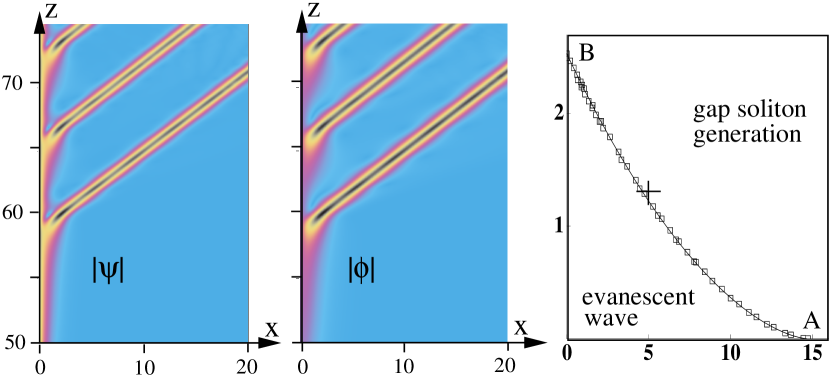
Figure 1: (color online) Left: intensity plots of a typical numerical simulation of the D3W system (Birefringent gap solitons.) with $\alpha=1.1$ subject to boundary conditions (2) with $A=5$, $B=1.3$ [the cross on the $(A,B)$ plot]. The maximum amplitudes of the emitted soliton are $|\psi|_{m}\sim 4.5$ and $|\phi|_{m}\sim 5.5$. Right: threshold curve in the $(A,B)$ plane where dots result from numerical simulations note-simuls and the curve is given by the solution of (6).

Let us consider a birefringent medium in permanent regime, namely assuming perfect frequency matching. In that case, degenerate spatial three-wave model (D3W) reduces to buryak majid

$$i\partial_{z}\psi+\frac{\alpha}{2}\partial_{x}^{2}\psi-\delta\psi+\phi^{2}=0,$$

$$i\partial_{z}\phi+\partial_{x}^{2}\phi+\psi\phi^{*}=0.$$ (1)

where $\phi(x,z)$ [respectively $\psi(x,z)e^{i\delta z}$] is the scaled static envelope of the signal wave with frequency $\omega$ and wave number $k$ [respectively second harmonic at frequency $\omega^{\prime}=2\omega$ and wave number $k^{\prime}$] and $\delta$ is the missmatch wavenumber in the propagation direction $z$ defined by $k^{\prime}=2k-\delta$. Last, $x$ is the transverse direction and $\alpha=1+\delta/k^{\prime}$ by definition. The system (Birefringent gap solitons.) is subject to the boundary condition

$$\psi(0,z)=Ae^{2iz},\quad\phi(0,z)=Be^{iz}$$ (2)

on the strip $x>0$, $z\in[0,L]$, with vanishing conditions as $x\to\infty$ and now with normalization $k^{\prime}=2$ (that is $\alpha=1+\delta/2$) note-BGS .

For the sake of simplicity, we only consider here the boundary conditions (2), although the wave number may in general be chosen different from $1$. We see on Fig.1 the generation, through the evanescent coupling, of birefringent gap solitons (BGS) formation and propagation above a threshold curve in the amplitude plane $(A,B)$. It is worth pointing out that the present situation is fundamentally different from studies of initial-value problems where field values are given at $z=0$, as, e.g., in the theoretical prediction leo-assanto and experimental realization canva for nondegenerate 3-wave interaction.

Asymptotic series solution.

Given the boundary values (2), we seek stationary solutions of the form

$$\psi(x,z)=u(x)e^{2iz},\quad\phi(x,z)=\sqrt{\alpha}\,v(x)e^{iz},$$ (3)

with real-valued functions $u$ and $v$ vanishing at infinity (the factor $\sqrt{\alpha}$ has been included for convenience). The system (Birefringent gap solitons.), now with $\delta=2(\alpha-1)$, provides for $u$ and $v$ the following parameter free equations

$$\partial_{x}^{2}u-4u+2v^{2}=0,\quad\partial_{x}^{2}v-v+uv=0,$$ (4)

Treating nonlinear terms as perturbative, we first solve the linearized equation for $v$ and obtain $v=\beta e^{-x}$. Substituting this result in the equation for $u$, we find that the $v^{2}$ term is resonant and generates a solution of the form $u=(\mu+\beta^{2}x/2)e^{-2x}$ where $\mu$ and $\beta$ are two arbitrary constants. This is the general solution of the quasilinear system $\partial_{x}^{2}u-4u+2v^{2}=0$, $\partial_{x}^{2}v=v$, that vanishes as $x\to\infty$.

The structure of (4) now indicates that $u$ and $v$ may be expressed as the following asymptotic series

$$u=\sum_{n=0}^{\infty}P_{n}(x)e^{-2(n+1)x},\quad v=\sum_{n=0}^{\infty}Q_{n}(x)e^{-(2n+1)x},$$

$$Q_{0}(x)=\beta,\quad P_{0}(x)=\mu+\beta^{2}x/2.$$ (5)

By inspection, the polynomials $P_{n}(x)$ and $Q_{n}(x)$ are of degree $n$ (except $P_{0}$ of degree 1) and obey a system of differential-recurrence equations obtained by replacing (Asymptotic series solution.) in (4). Their coefficients are then recursively given in terms of the two independent parameters $\beta$ and $\mu$. To ensure an accurate determination of the threshold curve, we have evaluated the first 17 terms of the series (Asymptotic series solution.), which takes up to a minute on a PC computer (with MAPLE or MATHEMATICA). The first ones are e.g. $Q_{1}=-3\beta^{3}/64-\mu\beta/8-\beta^{3}x/16$ and $P_{1}=\beta^{2}(24\mu+17\beta^{2})/576+x\beta^{4}/48$. The advantage of this method is to be applicable to any system driven in a forbidden band, which is essential when no soliton solution is known. Notice that, in the absence of resonant terms in the equations, the polynomials involved in the asymptotic series would simply be constants as e.g. in the Manakov system below.

NST threshold prediction.

Once the series (Asymptotic series solution.) has been determined up to a given truncation order $N$, imposing the boundary conditions $u(0)=A$ and $v(0)=B$ leads to the two driving amplitudes $A(\beta,\mu)$ and $B(\beta,\mu)$ explicitly expressed in terms of $\beta$ and $\mu$. Assuming that the supratransmission threshold curve is given by the maximum value of one of those, the other one being held constant, we can use a Lagrange parameter $\lambda$ and write the extremum condition as $\partial_{\mu}A-\lambda\partial_{\mu}B=0$ and $\partial_{\beta}A-\lambda\partial_{\beta}B=0$. This finally leads to the condition of vanishing Jacobian

$$J(\beta,\mu)=(\partial_{\beta}A)(\partial_{\mu}B)-(\partial_{\mu}A)(\partial_{\beta}B)=0.$$ (6)

With a high enough truncation order ($N=16$ here), the threshold curve is best obtained as the zero contour of the surface $J(\beta,\mu)$ plotted parametrically as a function of the amplitudes $A(\beta,\mu)$ and $B(\beta,\mu)$, as presented in Fig.1.

The condition (6) is symmetric with respect to $A$ and $B$, thus there is no need to specify which maximum amplitude is sought. Moreover condition (6) does not depend on the specific choice of parameters, provided they are independent. For instance, using the new parameters $\eta$ and $\sigma$ defined by

$$\beta=\exp(\eta),\quad\mu=(\sigma-\eta)\exp(2\eta),$$ (7)

the NST threshold condition becomes $J(\sigma,\eta)=0$. The interesting point here is that for fixed $\sigma$, the new parameter $\eta$ operates a shift of the solutions (Asymptotic series solution.) $u(x)\to u(x-\eta)$ and $v(x)\to v(x-\eta)$. Such a translation parameter always exists in systems that possess a translation invariance on the whole $x$-axis.

Generalizations.

Generalization of the procedure to $M$-component systems is straightforward. To this end, let us denote the components by $\phi_{m}(x,z)=u_{m}(x)e^{i\nu_{m}z}$ and their amplitudes by $u_{m}(0)=A_{m}(\{\eta_{n}\})$, where $\eta_{n}$ are the $M$ parameters of the solution (e.g. in the asymptotic solution). Finding the NST threshold manifold amounts to setting to zero the determinant of the Jacobi matrix of the amplitudes with respect to the parameters, that is

$${\rm det}\,[J_{mn}]=0,\quad J_{mn}=\frac{\partial A_{m}}{\partial\eta_{n}}.$$ (8)

To illustrate our result with another interesting problem, we may consider a multicomponent system having soliton solutions, the (integrable) Manakov system manakov , written here for spatial fields as

$$i\partial_{z}\psi+\partial^{2}_{x}\psi+2(|\phi|^{2}+|\psi|^{2})\psi=0,$$

$$i\partial_{z}\phi+\partial^{2}_{x}\phi+2(|\phi|^{2}+|\psi|^{2})\phi=0.$$ (9)

It possesses the two-parameter soliton solution note-NLS

$$\psi=e^{iz}\sin\theta\,{\rm sech\,}(x-\eta),\ \phi=e^{iz}\cos\theta\,{\rm sech\,}(x-\eta).$$ (10)

Subject then, on the semi-infinite strip $x>0$ and $z\in[0,L]$, to the boundary condition

$$\psi(0,z)=Ae^{iz},\quad\phi(0,z)=Be^{iz},$$ (11)

and vanishing values as $x\to\infty$, the Manakov system possesses solution (10) provided the parameters $(\eta,\,\theta)$ are related to the driving amplitudes $A$ and $B$ by

$$A=\sin\theta\,{\rm sech\,}\eta,\quad B=\cos\theta\,{\rm sech\,}\eta\ .$$ (12)

The threshold curve in the $(A,B)$ plane is then obtained by solving $J(\eta,\theta)=0$ as given by (6). The solution is $\eta=0$, that is, in the variables $(A,B)$, the circle $A^{2}+B^{2}=1$. This is illustrated on Fig.2 where we display a typical soliton formation and the NST threshold curve for which the points represent results of numerical simulations note-simuls .

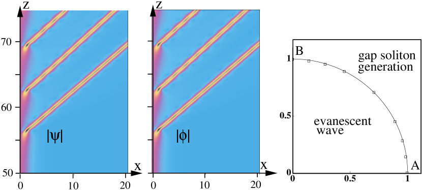
Figure 2: (color online) Left: typical numerical simulation of (Generalizations.) submitted to boundary conditions (11) with $A=0.45$ and $B=0.9$. The maximum amplitudes of the emitted soliton are $|\psi|_{m}\sim 1.2$ and $|\phi|_{m}\sim 2.3$. Right: threshold curve in the $(A,B)$-plane where the dots result from numerical simulations note-simuls and the curve is the circle $A^{2}+B^{2}=1$.

Then one can check that the threshold manifold of the $M$-component Manakov system, $i\partial_{z}\phi_{m}+\partial^{2}_{x}\phi_{m}+2(\sum_{1}^{M}|\phi_{n}|^{2})\phi_{m}=0$, subject to the boundary condition $\phi_{m}(0,z)=A_{m}e^{iz}$, is the $M$-dimensional sphere $\sum_{1}^{M}A_{m}^{2}=1$.

Parametric instability and supratransmission.

As can be seen from Figs.1 and 2, as soon as one of the amplitudes $A$ or $B$ crosses the threshold curve, the evanescent wave profile (soliton tail in integrable models) ceases to exist and gap solitons are emitted by the driven boundary. It turns out that, at least in the models we have investigated, the NST threshold manifold also corresponds to values of the parameters around which the stability of the solutions changes. To substantiate this claim, we investigate why the conditions for parametric and NST instabilities might indeed be the same by performing linear stability analysis of the stationary solutions (3) that we write in the form

$$\psi(x,z)=(u(x)+U(x,z))e^{2iz},$$ (13)

$$\phi(x,z)=\sqrt{\alpha}\,(v(x)+V(x,z))e^{iz}.$$ (14)

where $U$ and $V$ are small perturbations that satisfy, according to (2), the boundary condition

$$U(0,z)=0,\quad V(0,z)=0,$$ (15)

and vanishe at $x\rightarrow\infty$ for all $z$. Defining the real-valued perturbation vectors $\Gamma_{r}=(U_{r},V_{r})^{T}$ and $\Gamma_{i}=(U_{i},V_{i})^{T}$, where index $r$ ($i$) stands for real (imaginary) part, linearization of system (Birefringent gap solitons.) yields

$$\partial_{z}\Gamma_{r}+{\cal P}_{-}\Gamma_{i}=0,\quad\partial_{z}\Gamma_{i}-{\cal P}_{+}\Gamma_{r}=0.$$ (16)

The matrix differential operators ${\cal P}_{\pm}$ are given by

$${\cal P}_{\pm}=\left(\begin{array}[]{cc}\alpha&0\\ 0&1\end{array}\right)\left(\begin{array}[]{cc}\frac{1}{2}\partial_{x}^{2}-2&2v\\ v&\partial_{x}^{2}-1\pm u\end{array}\right).$$ (17)

This is conveniently written as an eigenvalue problem by differentiating with respect to $z$. For the real part $\Gamma_{r}(x,z)$ we may seek a solution $\Gamma_{r}(x,z)=\Phi_{\omega}(x)\cos(\omega z)$ and obtain

$${\cal P}_{-}{\cal P}_{+}\Phi_{\omega}=\omega^{2}\Phi_{\omega}$$ (18)

with boundary conditions (use $\partial_{z}\Gamma_{i}(0,z)=0$)

$$\Phi_{\omega}(0)=0,\quad({\cal P}_{+}\Phi_{\omega})(0)=0.$$ (19)

As ${\cal P}_{\pm}$ and $\Phi_{\omega}$ are real valued, $\omega^{2}$ is also real valued. Then the solution is linearly stable when $\omega^{2}>0$ and unstable for $\omega^{2}<0$, so that marginal instability is reached at the bifurcation point $\omega=0$ providing the parametric instability threshold.

An essential property of the operator ${\cal P}_{+}$, obtained by differentiation of (4) with respect to the parameters is

$${\cal P}_{+}\frac{\partial}{\partial\eta}\left(\begin{array}[]{c}u\\ v\end{array}\right)=0,\quad{\cal P}_{+}\frac{\partial}{\partial\sigma}\left(\begin{array}[]{c}u\\ v\end{array}\right)=0.$$ (20)

Thus a two-parameter family of solutions of (18) at $\omega=0$ reads

$$\Phi_{0}(x)=a\frac{\partial}{\partial\eta}\left(\begin{array}[]{c}u\\ v\end{array}\right)+b\frac{\partial}{\partial\sigma}\left(\begin{array}[]{c}u\\ v\end{array}\right),$$ (21)

for arbitrary constants $(a,b)\in\mathbb{R}^{2}$. Though it is not the most general solution of (18), it seems to be the only one able to satisfy the boundary conditions (19). Requiring then $\Phi_{0}(0)=0$, with $u(0)=A$ and $v(0)=B$, eventually yields $J(\eta,\sigma)=0$, namely the parametric instability condition (6). Thus the NST threshold condition (6), i.e., the condition for the maximum allowed amplitudes $A$ and $B$ at the boundary $x=0$, actually coincides with the onset of instability of the solution for the corresponding critical values of the parameters (here $\eta$ and $\sigma$).

To check this statement, we have computed numerically the eigenvalue $\omega^{2}$ of the differential equation (18) around the bifurcation point $\omega=0$ by varying $\eta$ and $\sigma$ around their critical values $\eta_{c}$ and $\sigma_{c}$ defined by the solution of $J(\eta,\sigma)=0$. The result is plotted in Fig.3 where we have used the asymptotic series solution $(u,v)$ at order $N=16$ as previously. As can be seen from the figure marginal instability is actually reached at the criticality ($\eta_{c}$ and $\sigma_{c}$) when $\omega$ crosses zero.

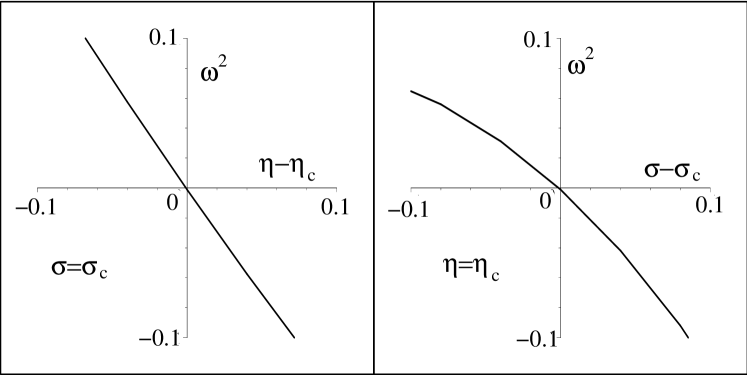
Figure 3: Plots of the eigenvalue $\omega^{2}$ in terms of the parameters $(\eta,\,\sigma)$ as a function of $\eta-\eta_{c}$ for $\sigma=\sigma_{c}$ (left) and function of $\sigma-\sigma_{c}$ for $\eta=\eta_{c}$ (right) again with $\alpha=1.1$.

Comments and conclusion.

The method presented here can be readily applied to the simple case of the scalar nonlinear Schrödinger equation $i\partial_{z}\psi+\partial^{2}_{x}\psi+2|\psi|^{2}\psi=0$ to get interesting insight about the occurrence of NST. It is found that (i) the asymptotic series solution actually sums up exactly to furnish the one-soliton solution, (ii) the fundamental parameter is the position $\eta$ of the soliton maximum, (iii) the threshold is indeed the maximum amplitude of this static soliton reached at $\eta=0$, (iv) the variations of the eigenvalue $\omega^{2}$ around zero is given by $\omega^{2}=-4\eta+o(\eta)$ that, straightforwardly, gives the marginal instability threshold $\eta=0$.

In such single component systems as NLS, the instability occurs always at the maximum amplitude of the solution note-max . On the contrary, the solution of the D3W model does not display any maximum nor any other geometric evidence that the NST threshold has been reached.

In conclusion, we have solved the challenging problem of determining the threshold for nonlinear supratransmission in nonintegrable $N$-component systems. This is obtained in two steps: first by deriving an asymptotic solution based on their linear evanescent profile that depends on $N$ parameters, and second by solving Eq. (8). In the parameter space the latter condition results in a $N-1$ dimensional manifold that determines the change of stability of the (asymptotic) solution. Expressed in terms of the amplitudes, it gives rise to the sought NST threshold. The situation is highly simplified in the case of an integrable system, or a system that possesses an exact static solitonlike solution, since one can work directly with the solution to obtain the threshold.

Finally, since no analytical expression is required, the method can be successfully applied to a wide class of nonintegrable nonlinear multicomponent systems.

- (1) F. Geniet, J. Leon, Phys Rev Lett 89 (2002) 134102
- (2) P. Maniadis, G. Kopidakis, S. Aubry, Physica D 216 (2006) 121
- (3) J. E. Macias-Daz, A. Puri, Phys Lett A 366 (2007) 447
- (4) J. Leon, A. Spire, Phys Lett A 327 (2004) 474
- (5) D. Taverner, N.G.R. Broderick, D.J. Richardson, R.I. Laming, M. Ibsen, Opt Lett 23 (1998) 328
- (6) R. Khomeriki, Phys Rev Lett 92 (2004) 063905
- (7) J. Leon, Phys Rev E 70 (2004) 056604
- (8) J. Leon, Phys Lett A 319 (2003) 130
- (9) H. Susanto, SIAM J Appl Math 69 (2008) 111
- (10) R. Khomeriki, J. Leon, Phys Rev Lett 94 (2005) 243902
- (11) See e.g. the review: A.V. Buryak, P. Di Trapani, D.V. Skryabin, S. Trillo, Phys. Rep. 370 (2002) 63-235
- (12) V.A. Brazhnyi, V.V. Konotop, S. Coulibaly, M. Taki, CHAOS 17 (2007) 037111
- (13) The points are obtained as follows: at fixed no soliton is emitted for some while at solitons are generated. The point is then set as and can be made as small as needed within the accuracy of the numerical code. As component profiles are initially set to zero, we smoothly increase amplitudes A and B from zero up to their respective assigned value to avoid shocks. This is why simulations are only displayed from on.
- (14) The driving wavenumber is scaled to any value by using the invariance D3W under the transformation , and .
- (15) G. Leo, G. Assanto, Opt. Lett. 22 (1997) 1391
- (16) M.T.G. Canva, R.A. Fuerst, S. Baboiu, G.I. Stegeman, G. Assanto, Opt. Lett. 22 (1997) 1683
- (17) S.V. Manakov, Sov Phys JETP 38 (1974) 248
- (18) The driving wavenumber is scaled to by using the invariance of the system under the transformation , and .
- (19) The NST condition (8) for a one-component system leads to that is to .