Comparing the efficiency of numerical techniques for the integration of variational equations

Abstract.

We present a comparison of different numerical techniques for the integration of variational equations. The methods presented can be applied to any autonomous Hamiltonian system whose kinetic energy is quadratic in the generalized momenta, and whose potential is a function of the generalized positions. We apply the various techniques to the well-known Hénon-Heiles system, and use the Smaller Alignment Index (SALI) method of chaos detection to evaluate the percentage of its chaotic orbits. The accuracy and the speed of the integration schemes in evaluating this percentage are used to investigate the numerical efficiency of the various techniques.

Enrico Gerlach

Lohrmann Observatory, Technical University Dresden, D-01062 Dresden, Germany

Charalampos Skokos

Max Planck Institute for the Physics of Complex Systems

Nöthnitzer Str. 38, D-01187 Dresden, Germany

(Communicated by the associate editor name)

1. Introduction

The determination of the stability of motion is of great importance when investigating nonlinear dynamical systems. To distinguish correctly between regular and chaotic motion, several different methods have been developed during the years. Most of these techniques, such as the maximal Lyapunov exponent [15], the fast Lyapunov indicator [4] or the Smaller Alignment Index (SALI) [14], rely on the study of the time evolution of deviation vectors from a given orbit to discriminate between the two regimes. The time evolution of these vectors is governed by the so-called variational equations.

Besides the correct determination of the regular or chaotic nature of individual orbits, in many cases, statistical statements over a large region of the phase space are also needed. For example, in order to determine the percentage of regular and chaotic orbits in a given system, the characterization of many orbits is required. In addition to the accurate computation of chaos indicators also for such tasks the CPU time needed to perform these computations becomes very important. In this work we compare different numerical techniques for the integration of the variational equations, concentrating on their accuracy and computational speed.

The paper is organized as follows: in section 2 we describe the general layout of our investigation. We concentrate our study on a simple two degrees of freedom Hamiltonian system: the well-known Hénon-Heiles system [7], which is presented in section 2.1. In our study we use the SALI method of chaos detection, which is presented in section 2.2. To solve the equations of motion of the Hénon-Heiles system and the associated variational equations one has to employ numerical methods. Any non-symplectic general-purpose integrator can be used for this task. In sections 2.3.1 and 2.3.2 we present two such techniques, which we use in our study. In [16] it was shown that it is also possible to use methods based on symplectic integration techniques to solve these equations. In section 2.3.3 we describe shortly the most efficient of these techniques: the so-called tangent map (TM) method. A numerical procedure to obtain relatively fast information on the nature of orbits for a large set of initial conditions is then given in section 2.4. In section 3 we present our numerical results for individual orbits, as well as global results for the whole system. The summary and the conclusions of our study are found in section 4.

2. Numerical integration of variational equations

2.1. Hénon-Heiles system

The Hamiltonian function of the Hénon-Heiles system [7] is

$$H(q_{1},q_{2},p_{1},p_{2})=\frac{1}{2}(p_{1}^{2}+p_{2}^{2})+\frac{1}{2}(q_{1}^{2}+q_{2}^{2})+q_{1}^{2}q_{2}-\frac{1}{3}q_{2}^{3},$$ (1)

with $q_{1}$, $q_{2}$ being the generalized coordinates and $p_{1}$, $p_{2}$ the conjugate momenta. The orbit evolution is given by the standard Hamilton equations of motion

$$\dot{q}_{i}=\frac{\partial H}{\partial p_{i}}\qquad\mathrm{and}\qquad\dot{p}_{i}=-\frac{\partial H}{\partial q_{i}},\qquad i=1,2,$$ (2)

where the dot denotes derivation with respect to time $t$. The time evolution of the variations $\delta q_{i},\delta p_{i}$ (which can be considered as coordinates of a deviation vector) is governed by the variational equations, given by

$$\dot{\delta q_{i}}=\delta p_{i}\qquad\mathrm{and}\qquad\dot{\delta p_{i}}=-\sum_{j=1}^{2}\frac{\partial^{2}H}{\partial q_{i}\partial q_{j}}\delta q_{j},\qquad i=1,2.$$ (3)

Eqs. (2) and (3) form a coupled system of ordinary differential equations. It should be noted that the solution of (3) depends explicitly on the solution of (2), i. e. on the reference orbit $q_{i}(t),p_{i}(t)$, and thus Eq. (3) cannot be solved independently from Eq. (2).

2.2. SALI method

The evaluation of the SALI is an efficient and simple method to determine the regular or chaotic nature of orbits in dynamical systems. The SALI was proposed in [14] has since been successfully applied in order to distinguish between regular and chaotic motion both in symplectic maps and Hamiltonian flows [17, 18, 13, 12, 3, 11, 19]. For the computation of the SALI of a given orbit, one has to follow the time evolution of the orbit itself and also of two deviation vectors $V_{1}(t),V_{2}(t)$, which initially point in two different directions. Then, according to [14] the SALI is defined as

$$SALI(t)=min\left\{\left\|\hat{V}_{1}(t)+\hat{V}_{2}(t)\right\|,\left\|\hat{V}_{1}(t)-\hat{V}_{2}(t)\right\|\right\},$$ (4)

where $\|\cdot\|$ denotes the usual Euclidean norm and $\hat{V}_{i}$, $i=1,2$ are normalized vectors with norm equal to 1.

The SALI has a completely different behavior for regular and chaotic orbits, and this allows us to clearly distinguish between them. In particular, the SALI fluctuates around a non-zero value for regular orbits, while it tends exponentially to zero for chaotic orbits [14, 17], following a rate which depends on the difference of the two largest Lyapunov exponents [18].

2.3. Used numerical methods

2.3.1. DOP853

The DOP853 integration method belongs to the big class of explicit Runge-Kutta methods. This non-symplectic scheme of order 8 is based on the method of Dormand and Price (see [5, Sect. II.5]). We use this integrator to solve the set of differential equations composed of Eqs. (2) and (3). Two free parameters, $\tau$ and $\delta$, are used to control its numerical performance. The first one defines the time span between two successive outputs of the computed solution. After each step of length $\tau$ the deviation vectors are renormalized and the value of SALI is computed. For the duration of each step $\tau$, the integrator adjusts its own internal time step in order to keep the local one-step error smaller than a user-defined threshold value $\delta$. For the DOP853 integrator the estimation of this local error and the step size control is based on embedded formulas of orders 5 and 3.

2.3.2. Taylor methods

The basic idea of the so-called Taylor series methods (for details see for example [5, Sect. I.8] and references therein) is to approximate the solution at time $t_{i}+\tau$ of a given $s$-dimensional initial value problem

$$\frac{\mathrm{d}\bm{y}(t)}{\mathrm{d}t}=\bm{f}(\bm{y}(t))\qquad\bm{y}\in\mathbb{R}^{s},\,t\in\mathbb{R}$$ (5)

from the $n$th degree Taylor series of $\bm{y}(t)$ at $t=t_{i}$ as

$$\bm{y}(t_{i}+\tau)\simeq\bm{y}(t_{i})+\tau\frac{\mathrm{d}\bm{y}(t_{i})}{\mathrm{d}t}+\frac{\tau^{2}}{2!}\frac{\mathrm{d}^{2}\bm{y}(t_{i})}{\mathrm{d}t^{2}}+\ldots+\frac{\tau^{n}}{n!}\frac{\mathrm{d}^{n}\bm{y}(t_{i})}{\mathrm{d}t^{n}}.$$ (6)

The computation of the derivatives is commonly done using automatic differentiation (see for example [8]).

In our study we use two different public available implementations of the Taylor method: TIDES [2] and TAYLOR [8]. Both methods have internal automatic order and step size computation to ensure the user-defined local one-step error $\delta$. Also here the parameter $\tau$ defines the step size, after which the renormalization of the deviation vectors and the computation of SALI is done.

The whole testbed of our work is written using the FORTRAN programming language exploiting extended double precision. While TIDES offers directly a FORTRAN integration routine, a wrapper to include the routine written in C had to be used for TAYLOR. Therefore for the latter only 16 significant digits were available for the integration.

2.3.3. TM method

Besides general-purpose integrators, it is also possible to use techniques based on symplectic methods to integrate the Hamilton equations of motion and the corresponding variational equations. This was shown in [16], where a thorough discussion of possible methods can be found. The most effective of these techniques, the TM method, is used in this work. Let us outline its basic idea, which is founded on a general result stated for example in [9]: Symplectic integrators can be applied to first order differential systems $\dot{X}=LX$, that can be written in the form $\dot{X}=(L_{A}+L_{B})X$, where $L,L_{A},L_{B}$ are differential operators defined as $L_{\chi}f=\{\chi,f\}$ and for which the two systems $\dot{X}=L_{A}X$ and $\dot{X}=L_{B}X$ are integrable. Here $\{f,g\}$ are Poisson brackets of functions $f(\bm{q},\bm{p})$, $g(\bm{q},\bm{p})$ defined as:

$$\{f,g\}=\sum_{l=1}^{N}\left(\frac{\partial f}{\partial p_{l}}\frac{\partial g}{\partial q_{l}}-\frac{\partial f}{\partial q_{l}}\frac{\partial g}{\partial p_{l}}\right).$$ (7)

The set of Eqs. (2) and (3) is one example of such a system, because Hamiltonian (1) can be divided into two integrable parts $A$ and $B$ with $H=A(\bm{p})+B(\bm{q})$. A symplectic integrator splits the equations of motion (2) into several parts, applying either the operator $L_{A}$ or $L_{B}$. These are the equations of motion of the Hamiltonians $A$ and $B$, which can be solved analytically, giving explicit mappings over the time step $c_{i}\tau$, where the constants $c_{i}$ are chosen to optimize the accuracy of the integrator. These mappings can then be combined to approximate the solution after time step $\tau$. In [16] it was shown that the derivative of these mappings - with respect to the coordinates and momenta of the system (the so-called tangent maps) - can be used for the time evolution of deviation vectors or, in other words, for solving the variational equations (3). We note that the TM method is called the ‘global symplectic integrator method’ in [10].

In [9] a family of symplectic integrators called SABA_n and SBAB_n was introduced, with $n$ being the number of applications of operators $L_{A}$ and $L_{B}$. These integrators have only positive intermediate steps and can be used with an additional corrector step $C$ at the beginning and the end of each step $\tau$ to increase their accuracy. An integrator of order 4 of this family, namely the SBAB₂C integrator which includes corrector steps, is used in our investigation. A detailed description of the application of the SBAB₂C integrator for the TM method to the Hénon-Heiles system can be found in [16].

2.4. Fast PSS method

Besides information on the chaotic or regular character of individual orbits, a more global description of dynamical systems is also of interest. For example, such a study could include the computation of the percentage of regular/chaotic orbits for a given set of initial conditions (ICs). This information requires the integration of the equations of motion/variational equations, and the computation of a chaos indicator for the whole set of ICs, which can become a very hard computational task. In order to address this problem, we implement a method proposed in [1], which exploits the Poincaré surface of section (PSS) of the system in order to speed up this computation.

For a fixed value of Hamiltonian (1) (throughout our study we use always $H=0.125$) we define the PSS of the system as the plane given by $q_{1}=0$ and $p_{1}\geq 0$. Each point in this plane defines a set of values ($q_{2},p_{2}$). To evaluate the percentage of regular orbits, one normally computes for each point the value of some chaos indicator using a dense set of points on the PSS as ICs. In Fig. 1 we consider a grid of $400\times 400$ ICs and color each one according to its SALI value at $t=3000$.

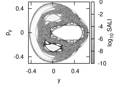
Figure 1. The PSS of the Hénon-Heiles system (1) for $q_{1}=0$ and $p_{1}\geq 0$. A grid of $400\times 400$ initial conditions is used and each initial condition is colored in grey-scale according to its SALI value at $t=3000$. Black dots forming five closed curves correspond to the regular orbit R1 of Fig. 2, while the scattered black dots are intersection points of the chaotic orbit C1 of Fig. 3 with the PSS.

Each orbit starting from any IC intersects the PSS in many points, and so, its SALI value can be attributed to all orbits having these intersection points as ICs. Therefore all these ICs do not have to be integrated separately. This procedure decreases drastically the CPU time needed for the global description of the system’s chaoticity. We refer to this approach as the fast PSS method.

3. Numerical results

3.1. Individual orbits

Let us first investigate, how well the different methods described in section 2.3 can determine the nature of individual orbits. We use these methods to integrate Eqs. (2) and (3), and then we compute the evolution of the SALI in order to determine the nature of the orbit. Unless otherwise stated, we always renormalize the deviation vectors after each time step of length $\tau=0.05$. For the non-symplectic routines we adopt a one-step accuracy of $\delta=10^{-5}$.

As representative examples we consider 3 orbits of the Hénon-Heiles system with different dynamical behaviors. The evolution of the SALI for a regular orbit (R1) is presented in Fig. 2, while in Fig. 3 we have similar results for a chaotic orbit (C1). Finally, in Fig. 4 the SALI of a sticky chaotic orbit (C2) is shown.

Figure 2. Time evolution of the SALI for the regular orbit R1 with initial conditions $q_{1}=0$, $p_{1}\approx 0.2334$, $q_{2}=0.558$, $p_{2}=0$.

Figure 3. Time evolution of the SALI for the chaotic orbit C1 with initial conditions $q_{1}=0$, $p_{1}\approx 0.4208$, $q_{2}=-0.25$, $p_{2}=0$.

Figure 4. Time evolution of the SALI for the sticky chaotic orbit C2 with initial conditions $q_{1}=0$, $p_{1}\approx 0.11879$, $q_{2}=0.335036$ and $p_{2}=-0.385631$.

From Fig. 2 we see that the results obtained for orbit R1 by the different integration methods are nearly identical. As theory predicts a constant SALI for regular motion, such behavior is correctly identified for orbit R1. Information concerning the numerical performance of various techniques for orbit R1 is given in Table 1 (throughout this paper the reported CPU times refer to an Intel Xeon X5660, 2.80 GHz computer). From the results reported in this table, we see that differences between the applied methods appear in their energy conservation properties, as is indicated by the relative energy error $|\Delta H/H|$, shown in Fig. 5. For the symplectic algorithm (TM method) $|\Delta H/H|$ shows fluctuations around $10^{-8}$, while it grows with time for the other methods as expected (see for example [6, Sect. IX.8]). The TAYLOR method has the worst performance since it is able to conserve the energy only up to an error level of $\approx 10^{-6}$ for $\delta=10^{-5}$. This is probably due to the 2 digits less in accuracy that are available for this method (see section 2.3). The best method with respect to the energy conservation is the TIDES algorithm for which the relative error is $\approx 10^{-13}$ ($\delta=10^{-5}$) and $\approx 10^{-16}$ ($\delta=10^{-16}$) at $t=10^{7}$. The price paid for the excellent accuracy of the algorithm is that TIDES requires, in general, the largest CPU times and the highest orders among the tested methods.

Table 1. Information on the performance of the different numerical methods used for the computation of the evolution of the regular orbit R1, of two deviation vectors from it and of its SALI. The step size $\tau$ was always 0.05. The order used by the TIDES and TAYLOR methods is determined by these routines for each step $\tau$ and is constant for the whole integration.

integrator	method	CPU time	Relative energy error	order
SBAB2C	TM	04m 02s	$2\times 10^{-8}$	4
DOP853	$\delta=10^{-5}$	09m 05s	$7\times 10^{-11}$	8
DOP853	$\delta=10^{-16}$	15m 58s	$1\times 10^{-11}$	8
TIDES	$\delta=10^{-5}$	15m 45s	$4\times 10^{-13}$	10
TIDES	$\delta=10^{-16}$	39m 39s	$1\times 10^{-16}$	23
TAYLOR	$\delta=10^{-5}$	15m 00s	$4\times 10^{-6}$	7
TAYLOR	$\delta=10^{-16}$	67m 01s	$4\times 10^{-13}$	20

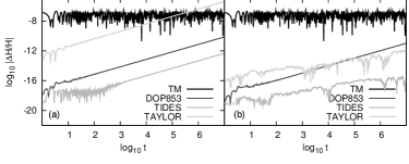
Figure 5. The time evolution of the relative energy error $|\Delta H/H|$ for the different integration schemes in the case of the regular orbit R1. The step size $\tau$ was 0.05 for all methods. For all non-symplectic methods we set (a) $\delta=10^{-5}$ and (b) $\delta=10^{-16}$. The relative energy error for the TM method is the same for both panels and is reported only for reference, since for this method no one-step accuracy $\delta$ is defined.

Orbit C1 is also correctly identified as chaotic by all methods in less than 1000 time units, within which SALI goes to zero (Fig. 3). A difference is found in the results for the sticky chaotic orbit C2 (Fig. 4). Up to $t\approx 10^{6}$ all methods indicate a regular behavior. It is only afterwards that SALI goes to zero for the TM, the DOP853 and the TIDES methods, correctly identifying C2 as a sticky chaotic orbit. For the used values of $\delta$ and $\tau$ the TAYLOR method does not succeed to show the decrease of SALI to zero, at least up to $t=10^{7}$.

3.2. Global results

In order to find the percentage of regular and chaotic orbits of the Hénon-Heiles system (1), we compute for a grid of $400\times 400$ ICs on the PSS the SALI value for different final times $t_{\mathrm{final}}$. One could argue that due to the finite resolution with which the grid of ICs is taken on the PSS, the fast PSS method (Sec. 2.4) would not be as accurate as the individual computation of SALI for each IC. The percentages (over the total number of ICs compatible with Hamiltonian (1)) of regular ($\mathrm{SALI}\geq 10^{-4}$), chaotic ($10^{-8}>\mathrm{SALI}$), and sticky chaotic orbits ($10^{-4}>\mathrm{SALI}\geq 10^{-8}$) obtained by both approaches using the TM method, are shown in Fig. 6(a), while the required CPU times are reported in Fig. 6(b). From the results of Fig. 6 we see that both approaches obtain practically the same values, while the CPU time needed by the fast PSS method remains considerably smaller with respect to the full integration of individual orbits. For this reason we apply the fast PSS method for computing the percentages of regular, chaotic and sticky chaotic orbits for different values of the time step $\tau$ and the final time $t_{\mathrm{final}}$. The obtained results can be found in Table 2.

Figure 6. (a) Percentage of regular, chaotic and sticky chaotic orbits as a function of $t_{\mathrm{final}}$, when each initial condition is integrated until time $t_{\mathrm{final}}$ (black dots) and when the fast PSS method was used (solid lines). The orbits are characterized according to their SALI value at time $t_{\mathrm{final}}$ as regular ($\mathrm{SALI}\geq 10^{-4}$), chaotic ($10^{-8}>\mathrm{SALI}$) and sticky chaotic ($10^{-4}>\mathrm{SALI}\geq 10^{-8}$). A grid of $400\times 400$ initial conditions on the PSS of Fig. 1 was used. The integrations of the orbit and the deviation vectors were done by the TM method using the SBAB₂C integrator with a step size $\tau=0.05$. (b) The CPU time needed for the computation of the results shown in (a).

Table 2. Percentage of regular, chaotic and sticky chaotic orbits for different values of the final time $t_{\mathrm{final}}$ and the step length $\tau$, for the integration schemes presented in section 2.3. A grid of $400\times 400$ initial conditions on the PSS of Fig. 1 is used. $\delta$ was set to $10^{-5}$ for the non-symplectic methods. The required CPU times are reported in the last column.

$\tau$	$t_{\mathrm{final}}$	method	% regular	% sticky chaotic	% chaotic	CPU time
0.50	$10^{4}$	TM	40.89	0.38	58.73	0 h 02 min
		DOP853	40.18	0.79	59.02	0 h 04 min
		TIDES	40.18	0.79	59.02	0 h 04 min
		TAYLOR	40.18	0.79	59.02	0 h 05 min
0.50	$10^{5}$	TM	40.05	0.07	59.88	0 h 09 min
		DOP853	39.71	0.37	59.92	0 h 14 min
		TIDES	39.22	0.49	60.29	0 h 17 min
		TAYLOR	40.19	0.47	59.34	0 h 15 min
0.50	$10^{6}$	TM	40.00	0.00	60.00	1 h 21 min
		DOP853	36.94	2.59	60.47	1 h 29 min
		TIDES	35.78	3.71	60.51	2 h 06 min
		TAYLOR	34.01	6.23	59.76	1 h 15 min
0.01	$10^{4}$	TM	40.38	0.72	58.90	0 h 19 min
		DOP853	40.22	0.70	59.08	0 h 38 min
		TIDES	40.22	0.70	59.08	1 h 05 min
		TAYLOR	40.23	0.84	58.93	0 h 59 min
0.01	$10^{5}$	TM	39.39	0.57	60.04	2 h 02 min
		DOP853	39.84	0.22	59.95	4 h 12 min
		TIDES	39.84	0.22	59.95	7 h 20 min
		TAYLOR	39.83	0.28	59.89	6 h 43 min
0.01	$10^{6}$	TM	40.01	0.00	59.99	19 h 26 min
		DOP853	40.02	0.28	59.70	39 h 42 min
		TIDES	40.02	0.28	59.70	68 h 08 min
		TAYLOR	39.95	0.21	59.84	62 h 32 min

From the results of Table 2 we see that for large values of $\tau$ and $t_{\mathrm{final}}$ ($\tau=0.50$ and $t_{\mathrm{final}}=10^{6}$) the non-symplectic methods find $3-4\%$ less regular orbits than the TM method. In order to understand this discrepancy we computed for orbit R1 the evolution of the SALI by the DOP853, the TIDES and the TAYLOR methods with $\tau=0.50$ and $\delta=10^{-5}$ (Fig. 7). From Fig. 7 we see that all non-symplectic methods fail to detect correctly the regular character of the orbit because SALI drops to zero after $t=10^{6}$. Such behaviors lead to the increase of the percentage of sticky chaotic orbits in Table 2, since some regular orbits are wrongly characterized as sticky or chaotic. Decreasing $\delta$ to values $\leq 10^{-14}$ solves the problem, as it leads to a correct identification of the orbit’s nature, but also increases the required CPU time (see Fig. 7).

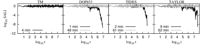
Figure 7. Time evolution of the SALI for the regular orbit R1 for $\tau=0.50$. For the DOP853, the TIDES and the TAYLOR non-symplectic methods we set $\delta=10^{-5}$ (black line) and $\delta=10^{-14}$ (grey line). The required CPU times are given as labels of the various lines.

For smaller values of $\tau$ the results obtained from different techniques are more consistent. For large integration times all methods give a similar percentage of regular orbits of $\approx 40\%$. TM, DOP853 and TIDES agree here within $0.01\%$. For $\tau=0.01$ and $t=10^{6}$ the TM method clearly discriminates between regular and chaotic orbits, while all other methods still find $\approx 0.3\%$ of sticky chaotic orbits. But since the SALI of those orbits will eventually go to zero as well, it can be expected that also the non-symplectic methods will give the same results as the TM method when the integration time is increased.

4. Summary and conclusions

We considered the problem of fast and accurate integration of the variational equations of a conservative Hamiltonian system. We compared different numerical techniques for this task, and applied them to the Hénon-Heiles system. We considered non-symplectic methods of high accuracy; particularly the DOP853 scheme, as well as the TIDES and TAYLOR packages, which are based on Taylor expansion techniques. We also applied the TM method, which exploits symplectic integrators, using in particular the SBAB₂C integrator.

The variational equations govern the evolution of small deviations from a given orbit. Using the SALI chaos indicator, which is defined through the time evolution of deviation vectors, we determined the chaotic or regular nature of individual orbits. In addition, applying an efficient numerical approach, the so-called fast PSS method, we were able to rapidly identify regions of order and chaos in the phase space of the system.

Our numerical results show that the TM method had the best numerical performance both in accuracy and in speed, especially for large integration steps, when the other non-symplectic schemes failed to compute accurately the fraction of regular and chaotic motion. For moderate integration steps all applied methods gave practically the same results, with the TM method being always faster.

Among the non-symplectic algorithms the TIDES was the most accurate one producing similar results as the DOP853 integrator. In many cases the results of the TAYLOR method were found to be less accurate than the ones obtained by the other methods, probably due to some implementation peculiarities of the algorithm.

Received xxxx 20xx; revised xxxx 20xx.

References

- [1] Ch. Antonopoulos, A. Manos and Ch. Skokos, SALI: an efficient indicator of chaos with application to 2 and 3 degrees of freedom Hamiltonian systems, in “Proc.of the 1st International Conference: From Scientific Computing to Computational Engineering” (ed. D.T. Tsahalis), Patras Univ. Press, (2005), 1292–1298.
- [2] (MR2121808) R. Barrio, Performance of the Taylor series method for ODEs/DAEs Appl. Math. Comput., 163 (2005), 525–545.
- [3] T. C. Bountis and Ch. Skokos, Application of the SALI chaos detection method to accelerator mappings, Nucl. Inst. Meth. Phys. Res. A, 561 (2006), 173–179.
- [4] (MR1472597) C. Froeschlé, and E. Lega and R. Gonczi, Fast Lyapunov Indicators. Application to Asteroidal Motion Cel. Mech. Dyn. Astron., 67 (1997), 41–62.
- [5] (MR1227985) E. Hairer, S. P. Nørsett and G. Wanner, “Solving Ordinary Differential Equations. Nonstiff Problems”, 2nd edition, Springer Series in Comput. Math., 1993.
- [6] (MR2221614) E. Hairer, C. Lubich and G. Wanner, “Geometric Numerical Integration. Structure-Preserving Algorithms for Ordinary Differential Equations”, Springer Series in Comput. Math., 2002.
- [7] (MR0158746) M. Hénon and C. Heiles, The applicability of the third integral of motion: some numerical experiments Astron. J., 69 (1964), 73–79.
- [8] (MR2146523) A. Jorba and M. Zou, A Software Package for the Numerical Integration of ODEs by Means of High-Order Taylor Methods, Experimental Mathematics, 14 (2005), 99–117.
- [9] (MR1864262) J. Laskar and P. Robutel, High order symplectic integrators for perturbed Hamiltonian systems, Cel. Mech. Dyn. Astr., 80 (2001), 39–62.
- [10] A.-S. Libert, C. Habaux and T. Carletti, Symplectic integration of deviation vectors and chaos determination. Application to the Hénon-Heiles model and to the restricted three-body problem., MNRAS, 414 (2011), 659–667.
- [11] (MR2479522) T. Manos, Ch. Skokos, E. Athanassoula and T. Bountis, Studying the global dynamics of conservative dynamical systems using the SALI chaos detection method Nonlin. Phenom. Complex Syst., 11 (2008), 171–176.
- [12] P. Panagopoulos, T. C. Bountis and Ch. Skokos, Existence and stability of localized oscillations in 1-dimensional lattices with soft spring and hard spring potentials J. Vib. & Acoust., 126 (2004), 520–527.
- [13] A. Széll, B. Érdi, Zs. Sándor and B. Steves, Chaotic and stable behavior in the Caledonian Symmetric Four-Body problem, MNRAS, 347 (2004), 380–388.
- [14] (MR1871759) Ch. Skokos, Alignment indices: A new, simple method for determining the ordered or chaotic nature of orbits, J. Phys. A, 34 (2001), 10029–10043.
- [15] Ch. Skokos, The Lyapunov Characteristic Exponents and their computation, in Lect. Notes Phys., 790 (2010), 63–135.
- [16] Ch. Skokos and E. Gerlach, Numerical integration of variational equations, Phys. Rev. E, 82 (2010), 036704.
- [17] Ch. Skokos, Ch. Antonopoulos, T.C. Bountis and M.N. Vrahatis, How does the Smaller Alignment Index (SALI) distinguish order from chaos?, Prog. Theor. Phys. Supp., 150 (2003), 439-443.
- [18] (MR2073606) Ch. Skokos, Ch. Antonopoulos, T.C. Bountis and M.N. Vrahatis, Detecting order and chaos in Hamiltonian systems by the SALI method, J. Phys. A, 37 (2004), 6269–6284.
- [19] P. Stránský, P. Hruška and P. Cejnar, Quantum chaos in the nuclear collective model: Classical-quantum correspondence, Phys. Rev. E, 79 (2009), 046202.