Probing the chiral regime of $N_{f}=2$ QCD with mixed actions

Abstract

We report on our first experiences with a mixed action setup with overlap valence quarks and non-perturbatively $\mbox{O}(a)$ improved Wilson sea quarks. For the latter we employ CLS $N_{f}=2$ configurations with light sea quark masses at small lattice spacings. Exact chiral symmetry allows to consider very light valence quarks and explore the matching to (partially quenched) Chiral Perturbation Theory (ChPT) in a mixed $\epsilon$/$p$-regime. We compute the topological susceptibility and the low-lying spectrum of the massless Neuberger-Dirac operator for three values of the sea quark mass, and compare the sea quark mass dependence to NLO ChPT in the mixed regime. This provides two different determinations of the chiral condensate, as well as information about some NLO low-energy couplings. Our results allow to test the consistency of the mixed-regime approach to ChPT, as well as of the mixed action framework.

I Introduction

Thanks to the theoretical and algorithmic improvements of recent years, and to the ever increasing computational power available, state-of-the-art Lattice QCD simulations now easily reach dynamical pion masses in the 200–300 MeV ballpark. In this mass region the effective description of the dynamics of pseudo-Goldstone bosons at low energies by means of chiral perturbation theory (ChPT) is expected to work well at a quantitative level. This gives rise to a fertile interaction: by matching Lattice QCD and ChPT results it is possible, on the one hand, to test the effective description vs. the fundamental theory; and, on the other hand, low-energy constants (LECs) can be determined from first principles, thus providing a sounder foundation to phenomenological applications of ChPT.

One particularly interesting aspect of the matching between QCD and ChPT is the role of finite volume effects Gasser and Leutwyler (1987a, b); Neuberger (1988a, b) (we will always assume that the theory lives in an Euclidean four-volume $V=L^{3}\times T$). While for large enough values of $L$ (one typical estimate is $M_{\pi}L\gtrsim 4$) the latter are expected to be strongly suppressed, and give rise only to small corrections to the infinite volume expansion in powers of pion momenta, the situation changes completely when the Compton wavelength of pions approaches $L$, i.e. $M_{\pi}L\sim 1$. In this regime slow pion modes, strongly affected by the finite volume, dominate the path integral in the effective theory, and the expansion in powers of $M_{\pi}^{2}/\Lambda_{\chi}^{2}$ breaks down. A new power-counting for this $\epsilon$-regime was proposed in Gasser and Leutwyler (1987b), which implies a rearrangement of the chiral expansion, in which quark mass effects are suppressed relative to volume effects. As a consequence, less LECs appear at any given order in the expansion relative to the infinite volume case, and the approach to the chiral limit is therefore more universal. This regime leads to a very different setup for the determination of LECs, which offers both the potential to obtain cleaner computations of some of the latter (those whose effects are unsuppressed in the quark mass), and a cross-check of the systematic uncertainties of “infinite” volume studies.

Another key property of finite volume chiral regimes ($\epsilon$-regime) is that the partition function of ChPT (at leading-order in the $\epsilon$-expansion) has been shown to be equivalent to a random matrix theory (RMT) Shuryak and Verbaarschot (1993); Verbaarschot and Zahed (1993); Verbaarschot (1994); Verbaarschot and Wettig (2000), where many analytical predictions can be obtained for spectral quantities, such the spectral density or the distribution of individual eigenvalues. These predictions are expected to be valid also for the spectrum of the Dirac operator in this regime, and have been tested both in quenched Edwards et al. (1999); Bietenholz et al. (2003); Giusti et al. (2003a), $N_{f}=2$ DeGrand et al. (2006); Lang et al. (2007); Fukaya et al. (2007a) and $N_{f}=2+1$ Hasenfratz et al. (2009); Fukaya et al. (2010) QCD. Since RMT predictions depend on one free parameter that corresponds to the chiral condensate (at the leading-order in the matching of ChPT and RMT), they provide yet another way of studying chiral symmetry breaking, using simple spectral observables.

As we will see the matching of ChPT in the $\epsilon$-regime holds up to NLO in the chiral expansion, both for full and partially-quenched (PQ) situations as long as some quarks remain in the $\epsilon$-regime, because the path integral is dominated by the zero-modes of the lighter pions. The matching of QCD to RMT can therefore be extended to unphysical situations which are however more favorable from the computational point of view.

Obviously enough, an adequate treatment of chiral symmetry on the lattice is especially relevant in this context. While simulations of $N_{f}=2(+1)$ QCD with full chiral symmetry have proven feasible, they are still limited to relatively small values of the inverse lattice spacing and/or physical volume Fukaya et al. (2009). A way to overcome this is to use a mixed action approach Bär et al. (2003, 2004), in which chiral symmetry is exactly preserved at the level of valence quarks only. Our aim is to develop such a framework by considering overlap valence quarks on top of $N_{f}=2$ Coordinated Lattice Simulations (CLS) ensembles, obtained from simulations with non-perturbatively $\mbox{O}(a)$ improved Wilson sea quarks.

We will use this method to study the matching of QCD to ChPT and RMT in a mixed regime, in which sea quark masses are in the $p$-regime and valence quark masses are in the $\epsilon$-regime Bernardoni and Hernández (2007); Bernardoni et al. (2008). From this matching we will be able to extract the $N_{f}=2$ low-energy couplings $\Sigma$ and $L_{6}$.

Furthermore, the use of overlap fermions allows us to measure the topological susceptibility of the dynamical Wilson configurations. The dependence of this quantity on the sea quark mass has been derived in ChPT at NLO in infinite volume in Chiu et al. (2009), and has been shown to depend on $\Sigma$ and on a combination of $L_{6}$, $L_{7}$ and $L_{8}$. We will show how this prediction can be easily obtained in the mixed regime of ChPT and we will test it from the measured distribution of the topological charge.

Obviously, mixed actions also have huge potential for phenomenological applications in which the exact preservation of chiral symmetry is greatly advantageous, e.g. to simplify the renormalisation of composite operators entering hadronic weak matrix elements. Along this line, first data for standard two- and three-point functions, as well as for correlation functions computed in the chiral limit via saturation with topological zero modes Giusti et al. (2004a); Hernández et al. (2008), will be covered in upcoming publications.

The structure of the paper is as follows. In Section II we review the main results from Bernardoni and Hernández (2007); Bernardoni et al. (2008) on the mixed-regime of ChPT and collect the results needed for our work, in which the sea quarks are degenerate and lie in the $p$-regime and valence quarks are in the $\epsilon$-regime. We will show that, up to NLO in the mixed-regime expansion, the partition functional matches onto a RMT, where the free parameter depends on the sea quark mass in a way that can be predicted from the matching. In Section  III we present our numerical results for the low-lying spectrum of the overlap operator and the topological susceptibility on Wilson sea quarks and compare with the predictions of RMT and ChPT. In Section  IV we present our results for the fits to ChPT predictions and extract the low-energy couplings.

II Probing the deep chiral regime with mixed actions

II.1 Mixed chiral regimes

While the exploration of chiral finite volume regimes ideally involves simulations with extremely light sea quarks, it is still possible to access them in a situation in which sea quarks have moderately larger masses.

The first step is to formulate ChPT in a so-called mixed regime Bernardoni and Hernández (2007); Bernardoni et al. (2008), in which $N_{s}$ quarks have masses such that the $p$-regime requirement $m_{s}\Sigma V\gg 1$ is satisfied, while $N_{l}$ quarks have masses that fulfill the $\epsilon$-regime condition $m_{l}\Sigma V\lesssim 1$. An appropriate power counting for this regime was first introduced in Bernardoni and Hernández (2007); Bernardoni et al. (2008):

$$p_{\mu}\sim{\cal O}(\epsilon),\;\;\;L,T\sim{\cal O}(1/\epsilon),\;\;\;m_{l}\sim{\cal O}(\epsilon^{4}),\;\;\;m_{s}\sim{\cal O}(\epsilon^{2}).$$ (1)

The partition function and meson correlators were computed to next-to-leading (NLO) order according to this power-counting, both in the context of fully dynamical quarks and also in various partially-quenched situations. The relevant PQ zero-mode integrals where also studied in Damgaard and Fukaya (2008). In this work, we want to keep the sea quarks in the $p$-regime and the valence quarks in the $\epsilon$-regime. We briefly describe the results for this situation, and we refer to the original papers for details on the computations.

As is common in the $\epsilon$-regime of PQChPT, we need to consider sectors of fixed topological charge. We will be dealing therefore with the replica method in which the PQ limit is obtained in the limit $N_{l}\rightarrow 0$.

The starting point is the parametrization of the Goldstone manifold according to the power-counting above. It can be shown that the non-perturbative zero-modes can be parametrized by a constant matrix, $\overline{U}_{0}\in U(N_{l})$ that together with various perturbative modes, $\xi(x),\bar{\eta}\sim{\mathcal{O}}(\epsilon)$ span the full Goldstone manifold ($\xi$ contains all the non-zero momentum modes, while $\bar{\eta}$ parametrizes the only perturbative zero-mode — for details see Bernardoni and Hernández (2007); Bernardoni et al. (2008)). The partition function in a sector of charge $\nu$ is given by Bernardoni and Hernández (2007); Bernardoni et al. (2008)

$$Z_{\nu}\simeq\int\left[d\xi\right]\left[d\bar{\eta}\right]\int_{U(N_{l})}\left[d\overline{U}_{0}\right]~{}J(\xi)~{}\det(\overline{U}_{0})^{\nu}\exp\left(-\int d^{4}x{\mathcal{L}}(\xi,\bar{\eta},\overline{U}_{0})\right).$$

$J(\xi)$ is the Jacobian associated with the parametrization Hansen (1990); Bernardoni and Hernández (2007); Bernardoni et al. (2008), and both the Lagrangian and the Jacobian can be perturbatively expanded in powers of $\xi$ and $\bar{\eta}$. The Lagrangian has an expansion in $\epsilon$ of the form:

$${\mathcal{L}} = \mathcal{L}^{(4)}+\mathcal{L}^{(6)}+...,$$ (3)

with terms up to $\mathcal{O}(\epsilon^{4})$, up to $\mathcal{O}(\epsilon^{6})$, etc , while $J(\xi)=1+{\mathcal{O}}(\epsilon^{2})$.

The leading-order Lagrangian is found to be:

$$\mathcal{L}^{(4)} \equiv {\rm Tr}\left[\partial_{\mu}\xi\partial_{\mu}\xi\right]-\frac{\Sigma}{2}{\rm Tr}\left[P_{l}\mathcal{M}P_{l}(\overline{U}_{0}+\overline{U}_{0}^{\dagger})\right]+{2\Sigma\over F^{2}}{\rm Tr}\left[P_{s}\mathcal{M}P_{s}\left(\xi-{F\over 2}{\bar{\eta}\over N_{h}}P_{s}\right)^{2}\right]+i{\nu\over V}\bar{\eta},$$

where $P_{l,s}$ are the projectors on the light and heavy quark sectors and $\mathcal{M}$ is the quark mass matrix. At this order, there is a factorization of the perturbative and non-perturbative modes.

An important observation from eq. (LABEL:eq:l4) is that the dependence on the non-perturbative modes, $\overline{U}_{0}$, and on the light quark mass is identical to that of a theory with $N_{l}$ quarks in the $\epsilon$-regime, but with the low-energy coupling, $\Sigma$, corresponding to a theory with $N_{f}=N_{l}+N_{s}$ flavours. This is to be expected since the heavier $p$-regime quarks behave, at the lowest energies, as decoupling particles that can be integrated out, but they are not quenched Bernardoni and Hernández (2007).

The quadratic form of the perturbative modes justifies their scaling with $\epsilon$. The last term in eq. (LABEL:eq:l4) could be treated as a perturbation as long as $\nu\sim\mathcal{O}(\epsilon^{0})$. However, in the partially-quenched case $N_{l}=0$ that we will be considering here, the distribution of topological charge is, on average, controlled by the sea quarks only. Indeed the $\nu$ dependence of the leading-order function is found to be (after integrating over the perturbative modes)

$$Z^{LO}_{\nu}\propto\exp\left(-{\nu^{2}\over VF^{2}}\sum_{s}{1\over M_{ss}^{2}}\right)\int_{U(N_{l})}\left[d\overline{U}_{0}\right]\det(\overline{U}_{0})^{\nu}\exp\left(\frac{\Sigma}{2}{\rm{Tr}}\left[P_{l}\mathcal{M}P_{l}(\overline{U}_{0}+\overline{U}_{0}^{\dagger})\right]\right),$$

(5)

where

$$M_{ss}^{2}\equiv{2m_{s}\Sigma\over F^{2}}.$$ (6)

In the case $N_{l}\rightarrow 0$, the integral over the zero-modes is exactly one (as in the quenched case) therefore all the $\nu$ dependence of the LO partition functional is in the explicit gaussian factor in eq. (5). The Leutwyler-Smilga result Leutwyler and Smilga (1992) for the topological susceptibility is obtained:

$$\langle\nu^{2}\rangle={1\over 2}VF^{2}{1\over\sum_{s}{1\over M_{ss}^{2}}}\sim\epsilon^{-2},$$ (7)

a scaling that makes the last term in eq. (LABEL:eq:l4) of $\mathcal{O}(\epsilon^{4})$, and therefore of leading order.

In fact we can easily push the computation of the topological susceptibility to NLO. In Mao and Chiu (2009); Aoki and Fukaya (2010), the topological susceptibility has been computed in ChPT to NLO when all the quarks are in the $p$-regime. The same result should be obtained in the mixed-regime case when $N_{l}\rightarrow 0$, since only the dynamical $p$-regime quarks can contribute to the distribution of topological charges when $N_{l}=0$. Indeed the NLO partition functional of ChPT in the mixed regime at fixed topology can be computed straightforwardly according to the power-counting rules of the mixed-regime, and the $\nu$ dependence can be explicitly determined. It turns out that for $N_{l}\rightarrow 0$, all the $\nu$-dependence comes from the integration of the perturbative modes $\xi$ and $\bar{\eta}$. The result for $N_{s}$ degenerate quarks is found to be

$$\langle\nu^{2}\rangle={m_{s}\Sigma V\over N_{s}} \left[1-{N_{s}^{2}-1\over N_{s}}\left({M_{ss}^{2}\over 16\pi^{2}F^{2}}\log\left({M_{ss}^{2}\over\mu^{2}}\right)+g_{1}(M_{ss},L,T)\right)\right.$$ (8)

$$+ \left.{16M_{ss}^{2}\over F^{2}}\left(L^{r}_{8}(\mu)+N_{s}L^{r}_{6}(\mu)+N_{s}L^{r}_{7}(\mu)\right)\right],$$

where the function $g_{1}(M,L,T)$ contains the finite volume corrections to the closed pion propagator; its explicit definition can be found in Hasenfratz and Leutwyler (1990). This result agrees with the NLO results of Mao and Chiu (2009); Aoki and Fukaya (2010). Note the appearance of $L_{7}^{r}(\mu)$, for which no prediction has yet been obtained on the lattice.

In Shuryak and Verbaarschot (1993); Verbaarschot and Zahed (1993); Verbaarschot (1994); Verbaarschot and Wettig (2000), it was shown that the $\epsilon$-regime zero-mode partition function at LO is that of a Random Matrix Theory (RMT) of matrices of size $N$, that depends only on the number of flavours, $N_{l}$, and the corresponding mass parameters $\hat{m}_{l}$, viz.

$$\int_{U(N_{l})}\left[dU\right]\det(U)^{\nu}\exp\left(\frac{\Sigma}{2}{\rm Tr}\left[\mathcal{M}(U+U^{\dagger})\right]\right)\simeq{\rm RMT}_{N}\{N_{l},\hat{m}_{l}\},$$ (9)

where ${\mathcal{M}}=\delta_{ij}m_{i}$ is the $N_{l}\times N_{l}$ mass matrix and there must be an identification $N\hat{m}_{i}=m_{i}\Sigma V$.

From this relation, the microscopic spectral density of the Dirac operator, as well as higher order spectral correlation functions, can be related to those quantities computed in the corresponding RMT. Furthermore, the distribution of individual low-lying eigenvalues of the massless Dirac operator can also be predicted from this equivalence Nishigaki et al. (1998); Damgaard and Nishigaki (2001); Akemann and Damgaard (2008), providing an efficient method to determine the chiral condensate, $\Sigma$. This relation has been tested in the quenched approximation and a good agreement has been found for volumes above $1.5$ fm or so Giusti et al. (2003a). In dynamical simulations, it has also been tested in DeGrand et al. (2006); Lang et al. (2007); Fukaya et al. (2007a) for $N_{f}=2$ and in Hasenfratz et al. (2009); Fukaya et al. (2010) for $N_{f}=2+1$. More details on the RMT formulation will be given in the Section II.2.

The rationale for expecting a matching of QCD to RMT relies on the existence of a regime where the chiral effective theory simplifies to a theory containing only the Goldstone zero-modes, as depicted in Fig. 1. In fact, if we consider ChPT in the usual $\epsilon$-regime or in the mixed-regime above, there is a hierarchy of scales $M_{vv}\ll L^{-1}$, which implies that we can integrate out the heavy scale $L^{-1}$ to obtain a theory of zero-modes only, which we could call ZMChT (zero-mode chiral theory). We can obtain this theory from the full ChPT integrating the heavy modes order by order in the $\epsilon$-expansion. The difference between doing this matching in the $\epsilon$ or the mixed-regime is the different assumption on the scaling of $M_{ss}$. In the former case, $M_{ss}\ll L^{-1}$ and this scale is not integrated out (the ZMChT has therefore $N_{l}+N_{s}$ flavours), while in the latter $L^{-1}\sim M_{ss}$ and the zero-modes of the sea pions must be integrated out as well (the ZMChT has then $N_{l}$ flavours).

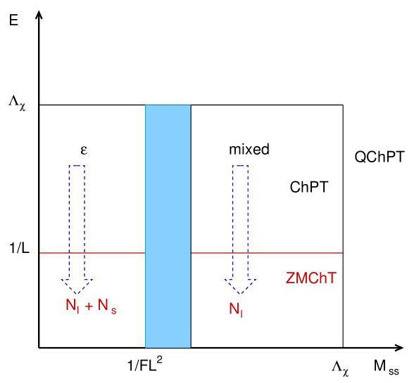
Figure 1: Chiral regimes of QCD showing the range of validity of the zero-mode chiral theory (ZMChT), which is equivalent to a RMT, and is obtained from ChPT by integrating out the non-zero momentum modes. $\Lambda_{\chi}\simeq 4\pi F$ represents the chiral symmetry breaking scale. The LECs of the ZMChT ($\Sigma_{\rm eff}$) can be derived from the LECs of ChPT from matching, which can be done in two regimes depending on the size of the sea quark mass. For $M_{ss}\ll 1/FL^{2}$, the $\epsilon$ regime is appropriate, while for $M_{ss}\geq 1/FL^{2}$ the mixed-regime has to be considered. The resulting ZMChTs have different number of flavours in the two cases.

.

The matching of ChPT and ZMChT at LO in the mixed-regime can be easily derived from eq. (LABEL:eq:l4): the ZMChT is simply ChPT at this order without the heavy modes (the integration over them gives an irrelevant normalization factor):

$$\left.Z_{\nu}^{ZMChT}\right|_{LO}\propto\int_{U(N_{l})}[d\overline{U}_{0}](\det\overline{U}_{0})^{\nu}\exp\left({\Sigma V\over 2}{\rm Tr}\left[P_{l}{\mathcal{M}}P_{l}\left(\overline{U}_{0}+\bar{U}^{\dagger}_{0}\right)\right]\right).$$ (10)

According to the eq. (9), this partition function is then equivalent to an $N_{l}$ RMT. In particular, it is important to stress that ZMChT has $N_{l}$ flavours, while the full ChPT from which it is derived corresponds to $N_{f}=N_{l}+N_{s}$ flavours. In particular, for $N_{l}\rightarrow 0$, the ZMChT or RMT we expect to find is the quenched one, while the couplings should be those of an $N_{f}=N_{s}$ theory.

The matching at NLO still does not modify the structure of the ZMChT theory. We could have anticipated this by realizing that there are no operators in the list of Gasser and Leutwyler that depend only on a constant $\overline{U}_{0}$ at ${\mathcal{O}}(\epsilon^{6})$. This does not mean however that there are no corrections, simply that they can be absorbed in the couplings appearing at LO in eq. (10), that is $\Sigma$. Indeed at NLO, there are corrections to the zero-mode Lagrangian from the ${\mathcal{O}}(p^{6})$ terms

$$\mathcal{L}^{(6)} = \ldots+{\Sigma\over F^{2}}{\rm Tr}\left[P_{l}\mathcal{M}P_{l}\left(\xi^{2}(x)\overline{U}_{0}+{\bar{U}}_{0}^{\dagger}\xi^{2}(x)\right)\right]$$

$$- 16{\Sigma L_{6}\over F^{4}}{\rm Tr}\left[P_{s}\mathcal{M}_{s}P_{s}\right]{\rm Tr}\left[P_{l}\mathcal{M}P_{l}\left(\overline{U}_{0}+{\bar{U}}_{0}^{\dagger}\right)\right]+\ldots.$$

The integrations over the $\xi,\bar{\eta}$ fields result in a change $\Sigma\rightarrow\Sigma_{\rm eff}$ Bernardoni et al. (2008),

$$Z_{\nu}^{ZMChT}|_{NLO}=\int_{U(N_{l})}[d\overline{U}_{0}](\det\overline{U}_{0})^{\nu}\exp\left({\Sigma_{\rm eff}V\over 2}{\rm Tr}\left[{\mathcal{M}}_{l}\left(\overline{U}_{0}+\bar{U}^{\dagger}_{0}\right)\right]\right),$$ (12)

with (for degenerate sea quarks)

$${\Sigma_{\rm eff}\over\Sigma}-1={1\over F^{2}}\left[16{L_{6}}N_{s}M^{2}_{ss}-{N_{l}}\bar{\Delta}(0)-{N_{s}}\Delta(M^{2}_{ss}/2)+\left({1\over N_{l}}\bar{\Delta}(0)-{N_{s}\over NN_{l}}\bar{\Delta}(M^{2}_{\eta})\right)\right],$$ (13)

where

$$M_{\eta}^{2}\equiv{N_{l}\over N_{f}}M_{ss}^{2}.$$ (14)

In dimensional regularization,

$$\Delta(M^{2})={M^{2}\over(4\pi)^{2}}\left(-\lambda+\log{M^{2}\over\mu^{2}}\right)+g_{1}(M,L,T),\;\;\;\;\;\bar{\Delta}(M^{2})=\Delta(M^{2})-{1\over VM^{2}},$$ (15)

and $\lambda$ contains the expected UV divergence

$$\lambda\equiv{1\over\epsilon}+\log 4\pi-\gamma+1-\log\mu^{2},\;\;\;\;\epsilon=2-d/2,$$ (16)

that gets fully subtracted in the usual $\overline{\rm MS}$ scheme. The small $M$ expansion of $\Delta$ gives

$$\Delta(M^{2})={1\over VM^{2}}+{M^{2}\over(4\pi)^{2}}\left(-\lambda-2\log{\mu L}\right)-\sum_{n=1}^{\infty}{1\over(n-1)!}\beta_{n}M^{2(n-1)}L^{2(n-2)},$$ (17)

where $\beta_{n}$ are the shape coefficients that depend only on the ratio $T/L$ Hasenfratz and Leutwyler (1990). Note that the $M\rightarrow 0$ limit of $\bar{\Delta}(M^{2})$ is well defined.

In summary, up to NLO we have found that the ZMChT is equivalent to a RMT. Furthermore, the matching of this theory with ChPT gives the precise dependence on the sea quark mass of the coupling $\Sigma_{\rm eff}$ which is the only free parameter of the RMT theory. Testing this prediction will be one of the main results of this work.

At this point it is interesting to discuss the possibility to have a smooth transition within the ZMChT regime between the $N_{f}=N_{l}+N_{s}$ effective theory and the $N_{l}$ theory as the scale $m_{s}$ is increased. The authors of Fukaya et al. (2007a) have assumed that indeed this is possible and have found some evidence that the eigenvalue ratios seem to follow the dependence on $m_{s}$ predicted by the RMT or ZMChT. Such expectation would be justified if the conditions were such that $FL\gg 1$, because in this case the scale $M_{ss}$ can be neglected in the integration of the non-zero modes, as is done in the $\epsilon$-regime. However this is not true in practice, where $FL\sim 1$, and indeed even though the eigenvalue ratios in Fukaya et al. (2007a) showed roughly the dependence on $m_{s}$ predicted by the RMT (note that $\Sigma_{\rm eff}$ drops in the ratios), this is certainly not true for the eigenvalues themselves. The mixed-regime matching is the correct procedure to account for the correct $m_{s}$ dependence of $\Sigma_{\rm eff}$, for large enough $m_{s}$. If $FL$ is not sufficiently large, there is no warranty that the transition region (vertical band in Fig. 1) can be modeled correctly by RMT. For a recent proposal to get predictions in the intermediate region from a resummation of zero-modes see Damgaard and Fukaya (2009).

The distribution of the lowest lying eigenvalues of the Dirac operator is expected to match the prediction of RMT with $N_{l}$ flavours and $\Sigma V\rightarrow\Sigma_{\rm eff}V$. $\Sigma_{\rm eff}$ depends on the low-energy couplings of the $N_{f}=N_{l}+N_{s}$ theory. Note that the only NLO coupling entering is $L_{6}$.

Now since we want to consider the case of quenched light quarks, we have to take the limit $N_{l}\rightarrow 0$. $\Sigma_{\rm eff}$ has a finite replica limit given by

$$\lim_{N_{l}\rightarrow 0}\Sigma_{\rm eff} \equiv \Sigma\,\Bigg{\{}1+{M_{ss}^{2}\over F^{2}}\Bigg{[}{\beta_{2}\over N_{s}}+{\log(\mu V^{1/4})\over 8\pi^{2}N_{s}}+16N_{s}L_{6}^{r}(\mu)-{N_{s}\over(4\pi)^{2}}\log\left({M_{ss}\over\sqrt{2}\mu}\right)\Bigg{]}$$ (18)

$$~{}~{}~{}~{}~{}~{}-{\beta_{1}\over N_{s}F^{2}\sqrt{V}}-{N_{s}\over F^{2}}g_{1}\left(M_{ss}/\sqrt{2},L,T\right)\Bigg{\}}.$$

For the case $T/L=2$, that we will be considering in our simulations, $\beta_{1}=0.08360$ and $\beta_{2}=-0.01295$. For details on how to compute the shape coefficients we refer to Ref. Hasenfratz and Leutwyler (1990). In Figure 2 we show the result of the ratio $\Sigma_{\rm eff}/\Sigma$ as a function of $M_{ss}^{2}/F^{2}$, for $N_{s}=2$, $F=90$ MeV and $L_{6}^{r}(M_{\rho})=0.07\cdot 10^{-3}$. The NLO corrections are quite significant, up to 30$\%$ for the masses considered.

Concerning the quenched limit of the zero-mode integral over $U(N_{l})$, a prescription using the supersymmetric or replica methods gives the well-known result for the quenched partition functional Splittorff and Verbaarschot (2003); Fyodorov and Akemann (2003) that matches quenched RMT (qRMT). The low-lying eigenvalues of the Dirac operator should then follow the predictions of qRMT. Comparing the eigenvalues computed numerically in this PQ setup with the predictions of qRMT, we can extract $\Sigma_{\rm eff}$ of eq. (18). If we do this for different values of the sea-quark mass, we can study the sea-quark mass dependence of $\Sigma_{\rm eff}$, from which we can in principle disentangle $\Sigma$ and $L^{r}_{6}(\mu)$, up to NNLO corrections (assuming we have an independent determination of $F$).

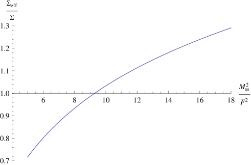
Figure 2: $\Sigma_{\rm eff}/\Sigma$ for $N_{f}=N_{s}=2$ as a function of $M^{2}_{ss}/F^{2}$ for $F=90$ MeV, $L_{6}^{r}(M_{\rho})=0.07\cdot 10^{-3}$.

A relevant question is however what are the eigenvalues that should be matched to RMT. Since there is a cutoff over which the ZMChPT should not be a good description, we expect that when the eigenvalues roughly reach such cutoff they should get significant corrections from the massive modes and therefore the matching to RMT should break up. A rough estimate would be the condition that $\lambda\leq m_{th}$, where $m_{th}$ is the value of the quark mass corresponding to the $p$-regime. For example taking the value of $m_{th}$ such that $ML\geq 3$, converts into the condition $\lambda\Sigma V\leq 9F^{2}LT/2$, which is roughly $6-7$ for our lattices. This results in the expectation that only the few lowest eigenvalues ($<3-4$ for our lattices) are below the threshold. For the largest eigenvalues , deviations from RMT could be sizeable, and the associated systematic uncertainty should be reduced by simulating at larger volumes.

II.2 Random matrix theory

We consider the gaussian chiral unitary model described by the partition function

$$\mathcal{Z}_{\nu}(\hat{m}_{1},...,\hat{m}_{N_{f}})=\int dWe^{-\frac{N}{2}{\rm Tr}(W^{\dagger}W)}\prod_{i=1}^{N_{l}}{\rm det}(\hat{D}+\hat{m}_{i}),$$ (19)

where

$$\hat{D}=\left(\begin{array}[]{cc}0&W\\ -W^{\dagger}&0\\ \end{array}\right),$$ (20)

and $W$ is a complex rectangular matrix of dimensions $(N+\nu)\times N$. Here $N$ plays the role of the space-time volume, multiplied by a constant. We are interested in the large-$N$ scaling limit at fixed $\mu_{i}=\hat{m}_{i}N$. The partition function $\mathcal{Z}_{\nu}$ then provides an equivalent description of the zero mode-chiral theory partition function in eq. (9) Shuryak and Verbaarschot (1993); Verbaarschot and Zahed (1993); Verbaarschot (1994); Verbaarschot and Wettig (2000) with $N_{l}$ flavours of mass $\hat{m}_{i}$ and fixed topological charge $\nu$, with the identification $N\hat{m}_{i}=m_{i}\Sigma V=\mu_{i}$.

If $x$ is the $k$-th smallest eigenvalue of the matrix $\sqrt{W^{\dagger}W}$, the probability distribution associated to the microscopic eigenvalue $\zeta=Nx$ can be written as

$$p_{k}^{\nu}(\zeta;\{\mu\})=\int_{0}^{\zeta}d\zeta_{1}\int_{\zeta_{1}}^{\zeta}d\zeta_{2}\dots\int_{\zeta_{k-2}}^{\zeta}d\zeta_{k-1}\omega_{k}^{\nu}(\zeta_{1},\dots,\zeta_{k-1},\zeta;\{\mu\}),$$ (21)

with $0\leq\zeta_{1}\leq\dots\leq\zeta_{k-1}\leq\zeta$. The explicit form of $\omega_{k}^{\nu}(\zeta_{1},\dots,\zeta_{k-1},\zeta;\{\mu\})$ is known in the microscopic limit Nishigaki et al. (1998); Damgaard and Nishigaki (2001). For instance, in the quenched case $N_{l}=0$ one has

$$\omega_{kq}^{\nu}(\zeta_{1},\dots,\zeta_{k-1},\zeta_{k};\{0\})=W_{k}^{\nu}e^{-\zeta_{k}^{2}/4}\zeta_{k}\prod_{i=1}^{k-1}\zeta_{i}^{2\nu+1}\prod_{k-1\geq i>j\geq 1}s(\zeta_{i},\zeta_{j})^{4}\times$$ (22)

$$Z_{2}(\underbrace{s(\zeta_{k},\zeta_{1}),s(\zeta_{k},\zeta_{1}),\dots,s(\zeta_{k},\zeta_{k-1}),s(\zeta_{k},\zeta_{k-1})}_{2(k-1)},\underbrace{\zeta_{k},\dots,\zeta_{k}}_{\nu}),$$

with

$$s(\zeta_{i},\zeta_{j})=\sqrt{\zeta_{i}^{2}-\zeta_{j}^{2}},$$ (23)

and

$$Z_{2}(s_{1},\cdots,s_{n})=\frac{{\rm det}A^{(n)}}{\Delta^{(n)}},$$

$$\left[A^{(n)}\right]_{ij}=s_{i}^{j-1}I_{j+1}(s_{i}),\;\;\Delta^{(n)}=\prod_{n\geq i>j\geq 1}(s_{i}^{2}-s_{j}^{2}),$$ (24)

where $I_{i}$ are modified Bessel functions. The coefficient $W_{k}^{\nu}$ can be fixed such that the probability $p_{k}^{\nu}$ is normalized to unity. There is an interesting property, called flavour-topology duality, which manifests itself at zero mass: $p_{k}^{\nu}(\zeta;\{0\})$ depends on the number of dynamical flavours and the topological charge only through the combination $\xi=N_{l}+|\nu|$. The microscopic spectral density

$$\rho_{S}^{\nu}(\zeta;\{\mu\})=\sum_{k=1}^{\infty}p_{k}^{\nu}(\zeta;\{\mu\})$$ (25)

coincides by construction with the one computed in the ZMChT Damgaard et al. (1999). For instance, the quenched LO spectral density is given by

$$\rho_{Sq}^{\nu}(\zeta;0)=\frac{\zeta}{2}\left[J_{\nu}(\zeta)^{2}-J_{\nu+1}(\zeta)J_{\nu-1}(\zeta)\right].$$ (26)

The equivalence can be extended to generic $n$-point density correlation functions. It is possible to show that probability distributions of single eigenvalues can be defined also in the chiral effective theory by means of recursion relations involving all spectral correlators Akemann and Damgaard (2004). The clear advantage of RMT is that the probability distributions are computable in practice, while in the chiral effective theory explicit expressions are missing. By assuming this equivalence holds for all spectral correlators, it is then legitimate to match the expectation values of the low eigenvalues of the massless QCD Dirac operator $\lambda_{k}$ with the predictions of the corresponding RMT.

We will be considering here a situation where two flavours of degenerate sea quarks have masses that are sufficiently large to be in the $p$-regime. In this case the sea quark mass does not appear explicitly in the ZMChT/RMT, as we have discussed. The latter corresponds to a theory with $N_{l}\rightarrow 0$ light flavours, that is quenched RMT (qRMT). The sea quark mass dependence comes in only through $\Sigma_{\rm eff}(M_{ss})$ and can be predicted at NLO, as explained in the previous section. Therefore we expect

$$\langle\zeta_{k}\rangle^{\nu}_{\rm qRMT}=\left.\Sigma_{\rm eff}(M_{ss})\right|_{N_{l}=0}V\langle\lambda_{k}\rangle^{\nu}_{\rm QCD}(M_{ss}),$$ (27)

where $M_{ss}$ is the sea pion mass, $\left.\Sigma_{\rm eff}(M_{ss})\right|_{N_{l}=0}$ is given in eq. (18), and expectations values are computed in RMT as

$$\langle\zeta_{k}\rangle^{\nu}_{\rm qRMT}=\int{\rm d}\zeta\,p_{k}^{\nu}(\zeta;0)\zeta.$$ (28)

In this matching we assume that the QCD quark masses, the eigenvalues of the Dirac operator and the quark condensate are properly renormalised. The prediction for the ratio $\langle\zeta_{k}\rangle^{\nu}_{\rm qRMT}/\langle\zeta_{l}\rangle^{\nu}_{\rm qRMT}$ is parameter-free and can be compared directly with $\langle\lambda_{k}\rangle^{\nu}_{\rm QCD}/\langle\lambda_{l}\rangle^{\nu}_{\rm QCD}$ at any fixed $M_{ss}$.

On the other hand, if we consider ratios at different sea quark masses of the form $\langle\lambda_{k}\rangle_{\rm QCD}^{\nu}(M_{1})/\langle\lambda_{k}\rangle_{\rm QCD}^{\nu}(M_{2})$, ($M_{1,2}$ are two different sea pion masses), we can assume that they can be matched to qRMT with appropriate values $\Sigma_{\rm eff}(M_{1,2})$ of the effective chiral condensate. Therefore

$$\frac{\langle\lambda_{k}\rangle_{\rm QCD}^{\nu}(M_{1})}{\langle\lambda_{k}\rangle_{\rm QCD}^{\nu}(M_{2})}=\frac{\langle\zeta_{k}\rangle^{\nu}_{{\rm qRMT}}}{\langle\zeta_{k}\rangle^{\nu}_{{\rm qRMT}}}\,\left.\frac{\Sigma_{\rm eff}(M_{2})}{\Sigma_{\rm eff}(M_{1})}\right|_{N_{l}=0}=\left.\frac{\Sigma_{\rm eff}(M_{2})}{\Sigma_{\rm eff}(M_{1})}\right|_{N_{l}=0}\,.$$ (29)

It follows that information on the mass dependence of $\Sigma_{\rm eff}$, and hence on $L_{6}$, can be obtained from suitable eigenvalue ratios.

III Results on Dirac spectral observables

$\beta=5.3$, $c_{\rm sw}=1.90952$, $V/a^{4}=48\times 24^{3}$
label	$\kappa$	$aM_{ss}$	$N_{\rm cfg}$
D4	0.13620	0.1695(14)	156
D5	0.13625	0.1499(15)	169
D6	0.13635	0.1183(37)	246	(D6a: 159, D6b: 87)

Table 1: Simulation parameters.

We have carried out our computations on CLS lattices of size $48\times 24^{3}$. The configurations have been generated with non-perturbatively $\mbox{O}(a)$ improved Wilson fermions at $\beta=5.3$ and sea quark masses given by $\kappa=0.13620,0.13625,0.13635$ Del Debbio et al. (2007a). The simulations have been performed with the DD-HMC algorithm Lüscher (2005); further details can be obtained in Del Debbio et al. (2007b). The lattice spacing has been determined to be $a=0.0784(10)~{}$fm in Del Debbio et al. (2007a), which implies that our lattices have physical size $L\simeq 1.88$ fm and sea pion masses of 426, 377 and 297 MeV, respectively. However, preliminary results from more precise determinations through different methods yield $a\simeq 0.070~{}$fm Brandt et al. (2010). We will consider both values in our analysis.

Following Del Debbio et al. (2007a), we will refer to our three lattices as D₄, D₅ and D₆. It has to be noted that for the D₆ lattice we have two statistically independent ensembles, that we dub D_6a and D_6b. We have analyzed 246 D₆ configurations, 169 D₅ configurations and 156 D₄ configurations; in all cases successive saved configurations are separated by 30 HMC trajectories of length $\tau=0.5$. In Table 1 we collect the simulation parameters. The sea pion masses in lattice units are taken from Del Debbio et al. (2007b) for the lattices D₄, D₅, while for D₆ we performed an independent evaluation from the pseudoscalar correlator computed on 96 CLS configurations. The resulting value implies $M_{\pi}L=2.84(9)$, which complies with the stability bound for the simulation algorithm derived in Del Debbio et al. (2006). On the other hand, $M_{\pi}L<3$ implies sizeable finite volume effects in p-regime physics, which in the present work are accounted for within ChPT.

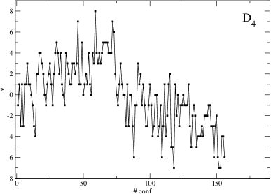
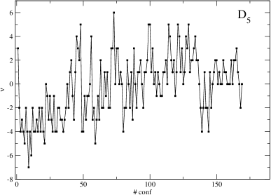
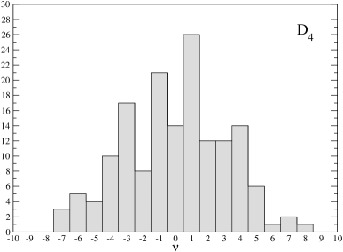
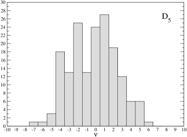
Figure 3: MC history and distribution of the topological charge in lattices D₄ and D₅.

On these configurations we have built the massless Neuberger-Dirac operator Neuberger (1998a, b)

$$D_{\rm N}=\frac{1}{\overline{a}}\left\{1+\gamma_{5}\;{\rm sign}(Q)\right\},$$ (30)

with

$$Q=\gamma_{5}(aD_{\rm W}-1-s),\;\;\;\;\overline{a}=\frac{a}{1+s},$$ (31)

where $D_{\rm W}$ is the Wilson Dirac operator. The parameter $s$ governs the locality of $D_{N}$ and has been fixed to $s=0.4$ for all our simulations. A discussion on the locality properties of the Neuberger-Dirac operator in our setup can be found in Appendix A.

Our Neuberger fermion code is the same used in previous quenched studies Giusti et al. (2003a, 2004b, 2007); Giusti and Necco (2007); Giusti et al. (2008), and is designed specifically to perform efficiently in the $\epsilon$-regime Giusti et al. (2003b). Our data analysis methods, including a discussion of autocorrelations in the observables under consideration, are discussed in Appendix B.

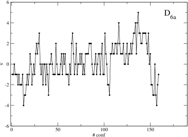
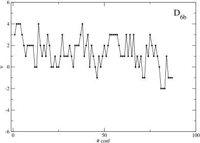
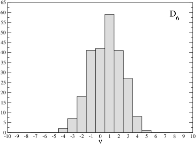
Figure 4: MC history and distribution of the topological charge in lattice D₆.

lattice	$\langle\nu\rangle$	$\langle\nu^{2}\rangle$
D4	0.01(55)	9.9(1.5)
D5	-0.24(40)	6.93(98)
D6	0.62(24)	3.36(47)

Table 2: Results for the expectation value of the topological charge and its square.

III.1 Topological charge

A first, immediate application of having constructed the Neuberger-Dirac operator $D_{\rm N}$ on a given dynamical configuration is the determination of the topological charge of the latter by computing the index of $D_{\rm N}$,

$$\nu=n_{+}-n_{-}$$ (32)

where $n_{+}$ ($n_{-}$) is the number of zero modes of $D_{\rm N}$ with positive (negative) chirality.

In the upper part of Figs. 3–4 we show the Monte Carlo history of the topological charge for our three lattices. The topology sampling proceeds smoothly, although there are clear hints at the presence of sizeable autocorrelations (cf. Appendix B). The histograms in the lower panels show the distribution of the measured topological charges, which qualitatively exhibits the expected Gaussian-like shape and width. This finding is consistent with the study reported in Schaefer et al. (2010), since our computations take place at a value of the lattice spacing sufficiently larger than the threshold $a\lesssim 0.05~{}{\rm fm}$ below which topology is expected to exhibit freezing symptoms.

In Table 2 we quote our results for the expectation values $\langle\nu\rangle$ and $\langle\nu^{2}\rangle$.

III.2 Low modes of the Dirac operator

We have computed the 10 lowest eigenvalues of the Neuberger-Dirac operator on lattices D₄, D₅ and D₆ by adopting the numerical techniques described in Giusti et al. (2003b).

The eigenvalues of $D_{\rm N}$ appear in general in complex conjugated pairs and lie on a circle in the complex plane

$$D_{\rm N}\psi=\gamma\psi,\;\;\;\;\gamma=\frac{1}{\overline{a}}(1-e^{i\phi}).$$ (33)

In order to compare them with the predictions of RMT, we have computed the projection Giusti et al. (2003a)

$$\lambda=\sqrt{\gamma\gamma^{*}}=\frac{1}{\overline{a}}\sqrt{2(1-\cos\phi)}.$$ (34)

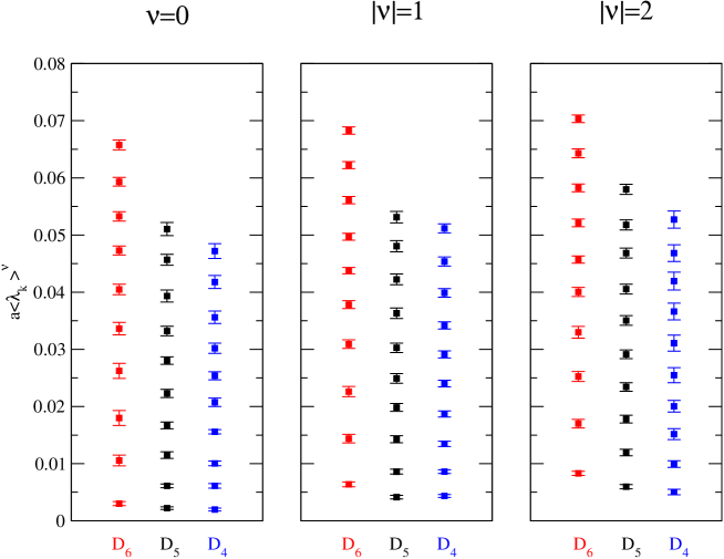
Figure 10: The first 10 bare low eigenvalues of the massless Neuberger operator at fixed topology $|\nu|=0,1,2$, for the three lattices D₄, D₅, D₆.

We have evaluated expectation values at fixed absolute value of the topological charge $|\nu|$. In Fig. 10 we show the bare eigenvalues for $|\nu|=0,1,2$.

Since the matching with RMT involves the parameter $\Sigma$, it is useful to first consider ratios of eigenvalues. In our case, following eq. (27), the QCD ratios $\langle\lambda_{k}\rangle^{\nu_{1}}/\langle\lambda_{l}\rangle^{\nu_{2}}$ can be directly matched with the qRMT predictions $\langle\zeta_{k}\rangle^{\nu_{1}}/\langle\zeta_{l}\rangle^{\nu_{2}}$. In Tables 7, 8 (App. B) we report the results for eigenvalue ratios involving the four lowest-lying eigenvalues and topologies $|\nu|=0,1,2$, together with qRMT predictions. It should be pointed out that the matching to RMT should work provided $\lambda_{k}\Sigma_{eff}V$ is not much larger that 1. For the lattice parameters we are considering, we set out cutoff at $k\leq 4$ for which the parameter is below 10. Since $k=4$ is probably borderline, we will not include it in the extraction of $\Sigma_{eff}$ though.

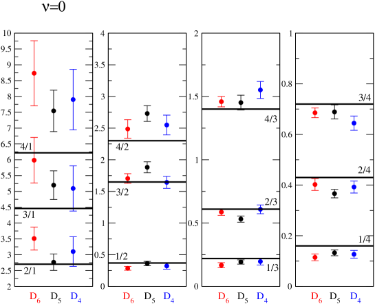
Figure 11: Eigenvalue ratios $\langle\lambda_{k}\rangle^{\nu}/\langle\lambda_{l}\rangle^{\nu}$ at fixed topological charge $\nu=0$. The horizontal lines represent the qRMT prediction.

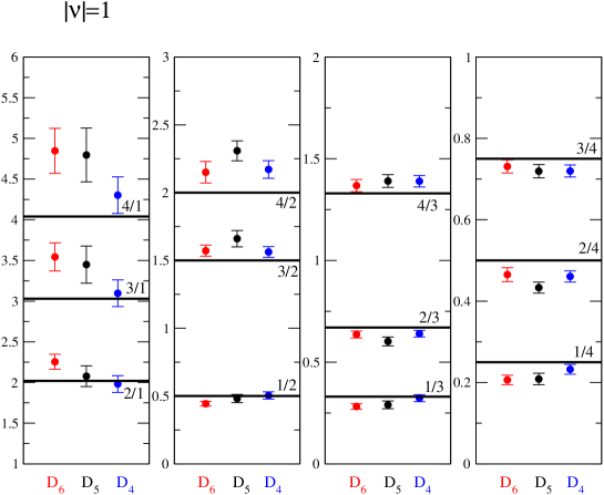
Figure 12: Eigenvalue ratios $\langle\lambda_{k}\rangle^{\nu}/\langle\lambda_{l}\rangle^{\nu}$ at fixed topological charge $|\nu|=1$. The horizontal lines represent the qRMT prediction.

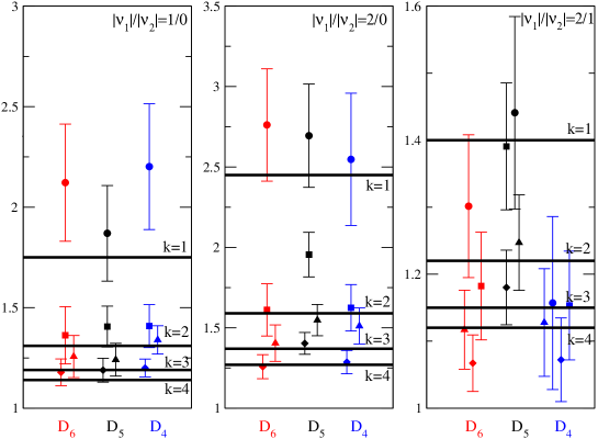
Figure 14: Eigenvalue ratios at fixed $k$, for different topological sectors. The circles correspond to $k=1$, the squares to $k=2$, the triangles to $k=3$ and the diamonds to $k=4$. The horizontal lines represent the qRMT prediction.

The ratios at fixed topological charge are shown in Figs. 11, 12, 13 (App. B); moreover, in Fig. 5 we report the ratios $\langle\lambda_{k}\rangle^{\nu}/\langle\lambda_{l}\rangle^{\nu}$ normalized to the corresponding qRMT predictions, for $|\nu|=0,1,2$ and for several combinations $k,l$ given in the bottom of the plot. This allows to appreciate clearly the precision and level of agreement with qRMT of each specific case. Finally, ratios at fixed $k$ involving different topological sectors are presented in Fig. 14 (App. B).

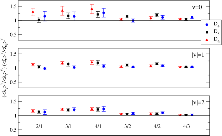
Figure 5: Eigenvalue ratios at fixed $|\nu|$, normalized to qRMT predictions, for the indices $(k,l)=(2,1),(3,1),(4,1),(3,2),(4,2),(4,3)$.

While the RMT prediction seems to work well for ratios not involving $\lambda_{1}$, the ratios $\langle\lambda_{k}\rangle/\langle\lambda_{1}\rangle$ exhibit somewhat more significant deviations. On the other hand, ratios between eigenvalues in different topological sectors follow well RMT predictions also in the case of $\lambda_{1}$, as shown in Fig. 14, albeit with larger errors. The data presented in this work do not allow for a full assessment of the systematics of these deviations, as this would require e.g. further values of the lattice spacing and/or physical volume. It is worth noting however that there are no clear differences between the three lattices, which we can take as an indication that corrections associated with relatively small values of $m_{s}$ are small. Concerning finite lattice spacing effects, having an estimate of the associated corrections in Wilson ChPT Sharpe and Singleton (1998); Rupak and Shoresh (2002); Bär et al. (2004) would be welcome, although our value of the lattice spacing is quite small. Finally, one has to keep in mind that the impact of autocorrelations on statistical errors cannot be estimated accurately for our ensembles. While we have attempted to stay on the safe side by quoting conservative errors that ought to include autocorrelations properly, it cannot be excluded that some errors are underestimated. Details are provided in App. B.

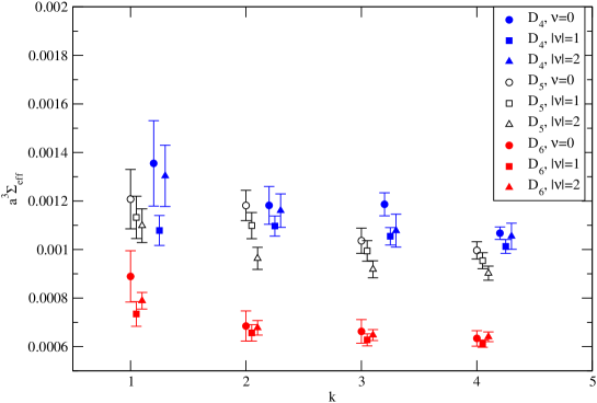
Figure 6: The bare effective condensate $\Sigma_{\rm eff}$ extracted from the matching in eq. (35), for $k=1,2,3,4$ and $|\nu|=0,1,2$. The data for D₄ have been shifted in the horizontal axis for better clarity.

III.3 Effective quark condensate

In the spirit of the mixed regime ChiPT analysis, our data also allow to study the mass dependence of the effective condensate, cf. eq. (29). In Table 9 we report the values of the bare effective condensate extracted from the matching

$$\Sigma_{\rm eff}(M_{ss})=\frac{\langle\zeta_{k}\rangle^{\nu}_{\rm qRMT}}{V\langle\lambda_{k}\rangle^{\nu}_{\rm QCD}}$$ (35)

for $k=1,2,3,4$ and $|\nu|=0,1,2$. The results are shown in Fig. 6, where one can observe that, at fixed value of the sea quark mass, $\Sigma_{\rm eff}$ does not depend on $k$ and $\nu$ within the statistical precision (with larger errors for $k=1$). By averaging over $k=2,3$ and $|\nu|=0,1,2$ we obtain

$$a^{3}\Sigma_{\rm eff} = 0.00113(3)(4)\;\;\;({\rm D}_{4}),$$

$$a^{3}\Sigma_{\rm eff} = 0.00103(3)(4)\;\;\;({\rm D}_{5}),$$ (36)

$$a^{3}\Sigma_{\rm eff} = 0.00066(2)(5)\;\;\;({\rm D}_{6}).$$

The first error is the statistical one, while the second uncertainty is a systematic effects estimated by adding the values for $k=1$ in the average. We have checked that including $k=4$ in the fit does not change the values within the statistical accuracy but decreases slightly the errors.

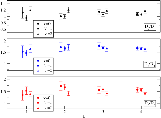
Figure 15: Ratios of eigenvalues at different sea quark masses, $\langle\lambda_{k}\rangle^{\nu}(M_{1})/\langle\lambda_{k}\rangle^{\nu}(M_{2})$, for $k=1,2,3,4$ and $|\nu|=0,1,2$.

Finally, in Fig. 15 (App. B) we show the ratios defined in eq. (29) for $k=1,2,3,4$ and $|\nu|=0,1,2$: they can be matched to the ratios of $\Sigma_{\rm eff}$ at different quark masses. Here we can see that, as expected, those ratios do not depend on the topology and on $k$, within the statistical uncertainties.

IV Fits to NLO Chiral Perturbation Theory

On the basis of the evidence presented in the previous section, now we assume that the matching to ChPT in the mixed-regime works in this range of sea quark masses and volumes, and try to extract the low-energy couplings from the sea-quark mass dependence of the two quantities $\Sigma_{\rm eff}$ and $\langle\nu^{2}\rangle$.

The NLO predictions from ChPT are summarized in eqs. (18) and (8). As expected they depend on the two leading order LECs, $\Sigma$ and $F$, but also on the ${\mathcal{O}}(p^{4})$ couplings $L_{6}$, $L_{7}$ and $L_{8}$.

Lattice	$am$	$am_{R}({\overline{\rm MS}},2\;{\rm GeV})$
D4	0.00954(8)	0.01366(23)
D5	0.00761(7)	0.01090(19)
D6	0.00445(22)	0.00637(33)

Table 3: Bare and renormalised ($\overline{\rm MS}$ scheme at 2 GeV) PCAC sea quark masses.

We first consider the topological charge distribution. The statistical error in this quantity is fairly large, but it is encouraging to see that there is a very clear dependence on the sea quark mass as shown in Fig. 7. We have fitted both to the full NLO formula in eq. (8), and to the linear LO behaviour. In either case $m_{s}$ is taken to be the PCAC Wilson mass renormalised in the $\overline{\rm MS}$ scheme at 2 GeV, tabulated in Table 3. The results for the lattice D₄ and D₅ are taken from Del Debbio et al. (2007b), while we have computed that of D₆, using the renormalization constants and improvement coefficients of Della Morte et al. (2005a); Della Morte et al. (2009); Della Morte et al. (2005b); Della Morte et al. (2008); Fritzsch et al. (2010).

At LO the slope provides a direct measurement of $\Sigma$ in the same scheme. At NLO we fit for $\Sigma$ and the combination $\left[L^{r}_{8}+2(L^{r}_{6}+L^{r}_{7})\right](M_{\rho})$ after fixing $\mu=M_{\rho}$ and rewriting $M_{ss}=2m_{s}\Sigma/F^{2}$. The value of $F$ is fixed to 90 MeV; the systematic uncertainty related to this choice is estimated by varying $F$ by $\pm 10$ MeV.

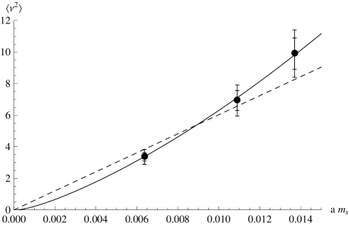
Figure 7: $\langle\nu^{2}\rangle$ versus the sea quark mass $am_{s}^{\overline{\rm MS}}(2{\rm GeV})$. The smaller errors are the statistical ones and the largest include our estimate of autocorrelations. The dashed and solid lines correspond to the best LO and NLO ChPT fits respectively (for $a=0.078$ fm).

In Table 4 we show the results of the LO and NLO fits. In the case of the NLO, there is a slight difference when the scale is taken to be $a=0.078~{}$fm Del Debbio et al. (2007a) or the preliminary result $a\simeq 0.070~{}$fm Brandt et al. (2010). We quote both. The $\chi^{2}$ is better for the NLO fit, but it is not possible to exclude the LO behaviour without decreasing our statistical errors. In physical units we get for $a=0.078-0.070~{}$fm:

$$\Sigma^{\overline{\rm MS}}(2\;{\rm GeV})=\left[262^{(33)(4)}_{(34)(5)}~{}{\rm MeV}\right]^{3}\;-\;\left[287^{(35)(5)}_{(36)(7)}~{}{\rm MeV}\right]^{3},\;\;\;$$ (37)

where the first error is coming out of the fit and the second is the effect of changing $F$.

	$\Sigma^{\overline{\rm MS}}(2\;{\rm GeV})a^{3}$	$[L^{r}_{8}+2(L^{r}_{6}+L^{r}_{7})](M_{\rho})$	$\chi^{2}/dof$
LO	0.00182(16)	-	1.2
NLO (a=0.078  fm)	0.00112(48)	0.0023(43)	0.02
NLO (a=0.070  fm)	0.00106(44)	0.0018(30)	0.03

Table 4: Results from the chiral fits to eq. (8).

There have been previous studies of the dependence on the topological susceptibility on the sea quark mass DeGrand and Schaefer (2007a); Aoki et al. (2008); Chiu et al. (2009); Bazavov et al. (2010), but as far as we are aware the fits in these works have not included the NLO chiral corrections.

Let us now turn to $\Sigma_{\rm eff}$. In this case, the dependence on $m_{s}$ is expected starting at NLO in ChPT. The results in the previous section indicate that indeed there is a significant sea quark mass dependence in this quantity. We perform a two-parameter NLO fit, where we fix $F$ and fit for $\Sigma$ and $L^{r}_{6}(M_{\rho})$. As a function of the $\overline{\rm MS}(2\;{\rm GeV})$ sea quark mass $m_{s}$, we expect therefore:

$$Z^{\overline{\rm MS}}_{S}\Sigma_{\rm eff}(m_{s}) = \Sigma\,\Bigg{\{}1+{2m_{s}\Sigma\over F^{4}}\Bigg{[}{\beta_{2}\over 2}+{1\over 16\pi^{2}}\log(M_{\rho}V^{1/4})+32L^{r}_{6}(M_{\rho})-{1\over 16\pi^{2}}\log\left({m_{s}\Sigma\over F^{2}M_{\rho}^{2}}\right)\Bigg{]}$$ (38)

$$~{}~{}~{}~{}~{}~{}-\frac{\beta_{1}}{2F^{2}V^{1/2}}-{2\over F^{2}}g_{1}\left(\sqrt{{\Sigma m_{s}\over F^{2}}},L,T\right)\Bigg{\}},$$

where we need the scalar density renormalization factor in the $\overline{\rm MS}$ scheme for the valence overlap fermions. We have obtained a rough estimate of this factor by matching our valence and sea sectors at a reference value of the pion mass, computed with mass-degenerate quarks, following the method of Hernández et al. (2001). We have done this at the unitary point on lattice D₅; choosing the latter instead of our lightest point D₆ allows to avoid sizeable finite volume effects in the determination of pion masses.

The sea pion mass in lattice units is $aM_{ss}=0.1499(15)$ Del Debbio et al. (2007b), while for the mass of the valence pion at bare valence quark mass $am=0.020$ we obtain $aM_{vv}=0.153(5)$ with 63 D₅ configurations. In order to obtain the renormalisation factor we then apply the matching condition

$$\left.\left(Z^{\overline{\rm MS}}_{\rm S}\right)^{-1}m\right|^{\rm overlap}_{M^{\rm ref}_{\pi}}=\left.m^{\overline{\rm MS}}(2~{}{\rm GeV})\right|^{\rm Wilson}_{M^{\rm ref}_{\pi}}$$ (39)

at $aM_{\rm ref}=aM_{ss}$. The renormalised $\overline{\rm MS}$ mass of the sea quark mass for the D₅ lattice can be read from Table 3, and we obtain

$$Z^{\overline{\rm MS}}_{\rm S}(2~{}{\rm GeV})=1.84(10),$$ (40)

where the error is dominated by the one in $aM_{vv}$, i.e. in the determination of the unitary point, and can be much improved with a larger statistics in the valence sector. Obviously, several checks need to be done to ensure that this result is robust, such as checking the dependence on the reference pion mass, as well as on the sea quark mass. A careful study of renormalization is beyond the scope of this exploratory study, and will be performed in a forthcoming publication.

With this estimate for the renormalisation factor and fixing $F=90$ MeV, the result we obtain from the fit is, for $a=0.078-0.070~{}$fm

$$\Sigma^{\overline{\rm MS}}(2\;{\rm GeV})a^{3} = 0.00102(18)-0.00099(16)\;\;\;$$ (41)

$$L_{6}^{r}(M_{\rho}) = 0.0015(11)-0.0010(7).$$ (42)

The quality of the fit is shown in Fig. 8. Although the fit is good, it would be desirable to have more sea quark masses and smaller statistical errors to assess the systematics of this chiral fit. Particularly useful would be to test the finite-size scaling.

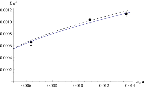
Figure 8: $\Sigma_{\rm eff}a^{3}$ as a function of the sea quark mass $am_{s}^{\overline{\rm MS}}(2{\rm GeV})$. The dashed and solid lines correspond to the best fit for $\Sigma$ and $L_{6}^{r}(M_{\rho})$ at $F=90~{}$MeV, taking the scale to be $0.070~{}$fm and $0.078~{}$fm respectively.

Translating to physical units we have

$$\Sigma^{\overline{\rm MS}}(2\;{\rm GeV})=\left[255^{(14)(1)}_{(16)(4)}~{}{\rm MeV}\right]^{3}\;-\;\left[280^{(14)(4)}_{(16)(5)}~{}{\rm MeV}\right]^{3},\;\;\;$$ (43)

where the only systematic error that has been estimated is that associated to the change of $F$ by $\pm 10$ MeV.

This value of $\Sigma$ is consistent with the one obtained from the topological susceptibility above, and both are in nice agreement with the alternative determination of Giusti and Luscher (2009), that extracted the condensate from the spectrum of the Wilson-Dirac operator on $N_{f}=2$ CLS configurations at the same lattice spacing and sea quark masses, but in a larger physical volume. A number of recent determinations of $\Sigma$ for $N_{f}=2$ can be found in the literature (for a recent review see Necco (2008)). The matching to ChPT has been done in the $p$-regime Noaki et al. (2008); Frezzotti et al. (2009); Baron et al. (2010), and also in the $\epsilon$-regime in Lang et al. (2007); DeGrand and Schaefer (2007b); Fukaya et al. (2007a, b); Hasenfratz et al. (2009, 2008). Our determination uses instead a PQ mixed regime and has been obtained with significantly finer lattices than the latter. Although our result lies in the same ballpark as many of these previous determinations, it is necessary to quantify the systematic uncertainties involved in our calculation. The dispersion of results for $\Sigma$ existing in the literature is rather disturbing, and it is very important to do a proper job at evaluating the systematic uncertainties: finite $a$, systematics of the chiral fits and finite-size scaling.

V Conclusions

We have implemented a mixed action approach to lattice QCD in which sea quarks are non-perturbatively $\mbox{O}(a)$ improved Wilson fermions, while valence quarks are overlap fermions. As a first application we have studied the spectrum of the Neuberger-Dirac operator, as well as the topological susceptibility, in the background of dynamical configurations at $a\approx 0.07~{}{\rm fm}$, for three values of the Wilson sea quark mass. The mixed-regime of ChPT provides predictions for these observables and their sea quark mass dependence in terms of various $N_{f}=2$ chiral low-energy couplings: at the NLO, they are $\Sigma$, $L_{6}$ and the combination $L_{8}+2(L_{6}+L_{7})$. We find that these NLO predictions describe our data well, and the extracted LECs are in good agreement with previous determinations.

This exploratory study obviously needs several important refinements to quantify systematic errors in a reliable way. Different volumes should be considered to test the expected finite-size scaling. Also, larger volumes will allow to augment the number of eigenvalues that can be safely matched to RMT predictions, which in turn will provide a definitive assessment of the associated systematic uncertainty. The lattice spacing is not known very precisely and an accurate determination is under way by various CLS groups. Obviously other $\beta$ values need to be considered to attempt a continuum extrapolation. Finally the effects of autocorrelations, that we have observed, would need larger statistics to ensure fully reliable statistical errors.

Our results show that new PQ setups where sea and valence quarks may lie in different chiral regimes ($p$ and $\epsilon$) are tractable (unphysical) regimes from which chiral physics can be extracted. Mixed actions are adequate to treat such regimes, and constitute an interesting approach for those applications where chiral symmetry plays an important role.

Appendix A Locality properties of the Neuberger-Dirac operator

The Neuberger-Dirac operator $D_{N}$ has been defined in eqs. (30), (31). While $Q$ is ultralocal, sign$(Q)=Q/(Q^{\dagger}Q)^{1/2}$ in general couples all space time points. As a consequence, the locality of the Neuberger-Dirac operator is not granted a priori. In Hernández et al. (1999) it was verified that locality is preserved in the quenched case, for values of the lattice spacing around and above the one we are considering now. We apply the method used there to our specific case.

We analyze the effect of the sign operator on a localized field $\eta$:

$$\psi(x)\equiv\mbox{sign(Q)}\eta(x)\qquad\eta_{\alpha}(x)=\delta_{xy}\delta_{\alpha 1}$$ (44)

where $y$ is some point on the lattice and $\alpha$ runs over the colour and the spin indices of the field. We evaluate the function:

$$f(r)\equiv\mbox{max}\{||\psi(x)||^{2}\mid||x-y||_{1}=r\}\,,$$ (45)

where $||\dots||_{1}$ denotes the so called “taxi-driver distance”. It is clear that locality is recovered in the continuum limit if $f(r)$ decays exponentially, with rate proportional to the cutoff $1/a$. To check that this indeed happens we fit the lattice data to $Ae^{-Br}$ in a range $r_{min}\leq r\leq r_{max}$. The upper limit has to be set because the inaccuracy with whom we calculate the overlap operator becomes bigger than the value of $f(r)$ at large enough distances.
The parameters of the simulation were set to calculate reliably $||\psi(x)||^{2}$ at least down to values of about $10^{-16}$ (corresponding to $r\sim 28$). However, as can be seen in Fig. 9, our implementation of the overlap operator is more precise and the picture of a decaying exponential only breaks down at $r\sim 38$ where $f(r)\sim 10^{-22}$.
We have taken in all the cases $r_{min}=14$ and $r_{max}=28$ also to compare with the results in Hernández et al. (1999). The parameter $s$ in eq. (31) can be varied to improve the locality properties of the Neuberger-Dirac operator. We collect the results of our fit for different values of $s$ in Table 5. The quoted error is obtained through jackknife with bin size 1. Among the values we adopted in our test, the choice $s=0.4$ yields the most satisfactory locality properties for this $\beta$ value, as shown in lower panel of Fig. 9. This result is in agreement with the previous studies in the quenched case. We will therefore adopt $s=0.4$ in our study.

s	$B$	$10^{4}$A	$\chi^{2}$
0.2	$0.711\pm 0.081$	$0.3\pm 0.1$	0.70
0.4	$1.001\pm 0.032$	$3.4\pm 1.5$	0.45
0.6	$0.975\pm 0.031$	$3.7\pm 1.2$	0.42

Table 5: Results of the fit for dynamical configurations after jackknife resampling. The results for $S=0.2,0.4,0.6$ are based respectively on a set of 13, 21, and 20 configurations, respectively.

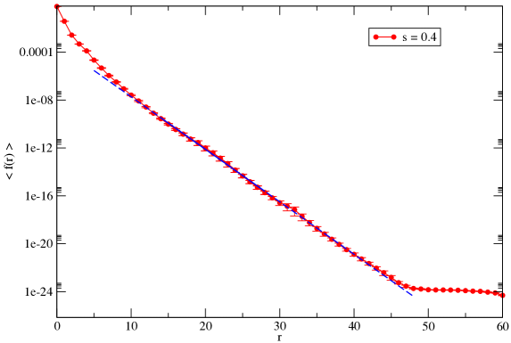
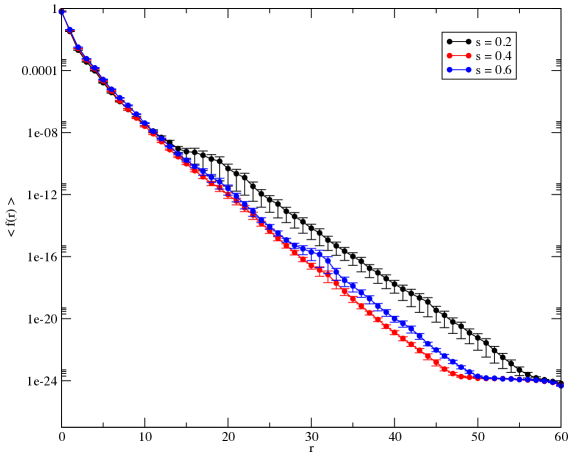
Figure 9: Upper panel: Result of the fit of $f(r)$ to $Ae^{-Br}$ for $s=0.4$. The blue line is the best fit to the data in the range $14\leq r\leq 28$. Lower panel: Comparison between various values of $s$.

Appendix B Statistical error analysis

B.1 Autocorrelations

We have studied the presence of autocorrelations in our observables in various ways:

• Integrated autocorrelation times have been estimated by using the methods described in Wolff (2004) and Lüscher (2005). In the first case, the summation window for the normalized autocorrelation function is fixed by setting the parameter $S$ of Wolff (2004) to $S=2$, while in the second case we stop the summation when the normalized autocorrelation function is zero within one sigma.

• The impact of changing the bin size in jackknife resampling of data has been assessed for all observables.

• The impact of autocorrelations on statistical errors has been estimated directly with the techniques described in Wolff (2004) for all observables (again with $S=2$).

In the case of the D₆ lattice, we have studied autocorrelations in the D_6a ensemble only, as considering it together with the independent D_6b ensemble would result in an underestimation of autocorrelation effects.

Our primary observables are the topological charge $\nu$ and expectation values of Dirac eigenvalues at fixed topology. In order to construct meaningful autocorrelation times for the latter, we consider their ratio with the RMT prediction for the expectation value of rescaled eigenvalues, i.e. $\langle\lambda_{k}\rangle_{\nu}/\langle\zeta_{k}\rangle_{{\rm RMT},\nu}=(\Sigma_{\rm eff}V)^{-1}$, which is $\nu$-independent up to higher orders in the $\epsilon$ chiral expansion. Results for autocorrelation times are given in Table 6. While uncertainties on $\tau_{\rm int}$ are remarkably large, due to the fact that measurements are performed only every 30 HMC trajectories, the values indicate that results coming from successive configurations are not completely decorrelated, especially in the case of the D₆ lattice.

	$\langle\nu\rangle$		$\langle\nu^{2}\rangle$
	$\tau_{\rm int}^{(1)}$	$\tau_{\rm int}^{(2)}$	$\tau_{\rm int}^{(1)}$	$\tau_{\rm int}^{(2)}$
D4	12.0(6.2)	8.0(5.2)	1.47(58)	0.83(12)
D5	6.4(3.4)	3.6(1.7)	1.7(0.7)	1.1(0.4)
D6a	4.9(2.5)	3.8(1.8)	2.9(1.3)	2.0(0.8)

	$\langle\lambda_{1}\rangle_{\nu}/\langle\zeta_{1}\rangle_{{\rm RMT},\nu}$		$\langle\lambda_{2}\rangle_{\nu}/\langle\zeta_{2}\rangle_{{\rm RMT},\nu}$		$\langle\lambda_{3}\rangle_{\nu}/\langle\zeta_{3}\rangle_{{\rm RMT},\nu}$		$\langle\lambda_{4}\rangle_{\nu}/\langle\zeta_{4}\rangle_{{\rm RMT},\nu}$
	$\tau_{\rm int}^{(1)}$	$\tau_{\rm int}^{(2)}$	$\tau_{\rm int}^{(1)}$	$\tau_{\rm int}^{(2)}$	$\tau_{\rm int}^{(1)}$	$\tau_{\rm int}^{(2)}$	$\tau_{\rm int}^{(1)}$	$\tau_{\rm int}^{(2)}$
D4	0.404(94)	$<0.5$	1.32(60)	$<0.5$	1.56(77)	$<0.5$	1.22(56)	$<0.5$
D5	0.56(15)	0.89(27)	1.45(63)	0.89(27)	0.93(34)	0.89(27)	1.22(54)	0.89(27)
D6a	2.7(1.3)	2.3(1.1)	4.0(2.1)	3.2(1.5)	7.0(3.9)	4.4(2.4)	7.4(4.0)	5.2(3.2)

Table 6: Estimated autocorrelation times for the topological charge and its square (upper panel), as well as for the ratios $\langle\lambda_{k}\rangle_{\nu}/\langle\zeta_{k}\rangle_{{\rm RMT},\nu}$ up to $k=4$ (lower panel). Superindices $(1)$ and $(2)$ refer to computations following Wolff (2004) and Lüscher (2005), respectively. $\tau_{\rm int}$ is provided in units of gauge configurations, i.e. it should be multiplied times $30$ to convert to number of trajectories and times $15$ to convert to MC time.

This is further reinforced by the analysis of the dependence of jackknife errors on the bin size. Again, this exercise is constrained by limited statistics, as the number of available configurations decreases rapidly with increasing $|\nu|$. Still, for topologies $|\nu|=0,1,2$ it is possible to have meaningful errors up to bin sizes of at least 5 configurations on lattices D₅ and D₆. On lattice D₅, errors for $\langle\lambda_{k}\rangle_{|\nu|}$ and ratios $\langle\lambda_{k}\rangle_{|\nu|}/\langle\lambda_{j}\rangle_{|\nu|}$ exhibit little or no dependence on the bin size, with errors increasing by at most 20 to 30%. On the other hand, on lattice D₆ errors consistently increase with the bin size, and, in cases where there is enough statistics to avoid an early loss of signal, they tend to saturate around bin sizes of the order of 3–4, at which point they are between 30% and 70% larger than with bin size 1. Finally, the errors taking into account autocorrelations computed following Wolff (2004) are consistent with jackknife errors with bin size 1 on D₅, while on D₆ they are systematically consistent with those around which the jackknife bin dependence stabilizes, and in some cases even slightly larger.

Regarding the topological charge, where statistics allows to trace the bin size dependence up to much larger values, the increase in the error of $\langle\nu\rangle$ and $\langle\nu^{2}\rangle$ is much more marked than for Dirac eigenvalues. Typically, jackknife errors stabilize for bin sizes between 5 and 10 for all three lattices, at which point they are larger by as much as 60% with respect to those for bin size 1. The analysis à la Wolff (2004) yields comparable errors.

Our conclusion is that there is evidence that autocorrelations affect the topological charge in all three lattices, while spectral observables are affected by detectable autocorrelations on D₆ only. As a simple recipe to stay on the safe side when including autocorrelation effect in the errors, we quote results for spectral observables from the analysis with jackknife bin size 1 for lattices D₄ and D₅ and bin size 3 for lattice D₆. In the case of $\langle\nu\rangle$ and $\langle\nu^{2}\rangle$ we quote jackknife errors for the bin sizes at which they stabilize. It has to be stressed that we find no significative evidence that autocorrelations depend on the sea quark mass in some systematic way.

B.2 Systematic errors in the computation of Dirac eigenvalues

The numerical computation of eigenmodes and eigenvalues of the Hermitian non-negative operator $D_{\rm N}^{\dagger}D_{\rm N}$ has been performed with the techniques described in Giusti et al. (2003b). The accuracy to which eigenmodes are computed is bound by an input parameter, which in our case has been set to 1% in lattices D₄ and D₅ and 5% in lattice D₆. On the other hand, for each separate eigenmode an a posteriori estimate of the actual error in the computation of the eigenvalue is produced by the program. Usually, this estimate yields an error one order of magnitude smaller than the nominal accuracy parameter mentioned above.

This systematic error should, in principle, be added in quadrature to the statistical error of $\langle\lambda_{k}\rangle$ and observables derived thereof. We have estimated its impact, and found that it is completely negligible with respect to statistical errors in lattices D₄ and D₅, both if it is computed using the estimates on each eigenvalue accuracy and in the much more pessimistic case in which a flat error associated to the 1% nominal precision is set. In the case of D₆, the uncertainty coming from numerical error estimates is again negligible, but a flat error set at 5% yields uncertainties comparable to the statistical ones. However, our experience shows that the estimates produced by the program are in the right ballpark, and conclude that setting a flat 5% uncertainty in D₆ observables would be a gross overestimate of the effect. Hence, we have opted for neglecting this source of error in our final results.

$|\nu|$	$k/l$	D4	D5	D6	qRMT
0	2/1	3.10(47)	2.76(26)	3.51(36)	2.70
0	3/1	5.09(71)	5.20(45)	5.98(72)	4.46
0	4/1	7.89(96)	7.54(65)	8.7(1.0)	6.22
0	3/2	1.64(9)	1.88(9)	1.70(8)	1.65
0	4/2	2.55(16)	2.73(12)	2.49(15)	2.30
0	4/3	1.55(7)	1.45(6)	1.46(4)	1.40
1	2/1	1.98(10)	2.08(13)	2.26(10)	2.02
1	3/1	3.10(16)	3.45(23)	3.56(19)	3.03
1	4/1	4.30(23)	4.80(33)	4.85(30)	4.04
1	3/2	1.56(4)	1.66(6)	1.57(4)	1.50
1	4/2	2.17(6)	2.31(7)	2.15(8)	2.00
1	4/3	1.39(3)	1.39(3)	1.36(3)	1.33
2	2/1	1.98(15)	2.00(10)	2.04(8)	1.76
2	3/1	3.02(21)	2.99(16)	3.02(10)	2.50
2	4/1	3.99(28)	3.93(20)	3.94(14)	3.23
2	3/2	1.53(5)	1.49(4)	1.48(4)	1.42
2	4/2	2.02(7)	1.96(6)	1.93(7)	1.83
2	4/3	1.32(5)	1.32(2)	1.30(3)	1.29

Table 7: Results for eigenvalue ratios at fixed topology $\langle\lambda_{k}\rangle^{\nu}/\langle\lambda_{l}\rangle^{\nu}$ compared with qRMT predictions $\langle\zeta_{k}\rangle^{\nu}/\langle\zeta_{l}\rangle^{\nu}$.

$k$	$|\nu_{1}|/|\nu_{2}|$	D4	D5	D6	qRMT
1	1/0	2.20(31)	1.87(24)	2.12(29)	1.75
2	1/0	1.41(11)	1.41(10)	1.36(14)	1.31
3	1/0	1.34(7)	1.24(8)	1.26(10)	1.19
4	1/0	1.20(4)	1.19(6)	1.18(7)	1.14
1	2/0	2.55(41)	2.69(32)	2.76(35)	2.45
2	2/0	1.62(14)	1.96(14)	1.61(16)	1.59
3	2/0	1.51(11)	1.55(10)	1.40(11)	1.37
4	2/0	1.29(7)	1.40(7)	1.26(7)	1.27
1	2/1	1.16(13)	1.44(14)	1.30(11)	1.40
2	2/1	1.15(8)	1.39(9)	1.18(8)	1.22
3	2/1	1.13(8)	1.25(7)	1.12(6)	1.15
4	2/1	1.07(6)	1.18(6)	1.07(4)	1.12

Table 8: Results for eigenvalue ratios $\langle\lambda_{k}\rangle^{\nu_{1}}/\langle\lambda_{k}\rangle^{\nu_{2}}$ compared with qRMT predictions $\langle\zeta_{k}\rangle^{\nu_{1}}/\langle\zeta_{k}\rangle^{\nu_{2}}$.

$k$	$|\nu|$	$a^{3}\Sigma_{\rm eff}$(D4)	$a^{3}\Sigma_{\rm eff}$(D5)	$a^{3}\Sigma_{\rm eff}$(D6)
1	0	0.00135(18)	0.00121(12)	0.00089(11)
2	0	0.00118(8)	0.00118(6)	0.00068(6)
3	0	0.00119(5)	0.00104(5)	0.00066(5)
4	0	0.00107(3)	0.00100(4)	0.00063(3)
1	1	0.00108(6)	0.00113(9)	0.00074(5)
2	1	0.00110(4)	0.00110(5)	0.00066(3)
3	1	0.00105(4)	0.00099(4)	0.00063(2)
4	1	0.00101(3)	0.00095(3)	0.00061(1)
1	2	0.00130(13)	0.00110(7)	0.00078(2)
2	2	0.00116(7)	0.00096(5)	0.00068(3)
3	2	0.00108(7)	0.00092(4)	0.00065(2)
4	2	0.00105(5)	0.00090(3)	0.00064(2)

Table 9: The bare effective condensate $\Sigma_{\rm eff}$ extracted from the ratios $\langle\zeta_{k}\rangle^{\nu}_{\rm qRMT}/(V\langle\lambda_{k}\rangle^{\nu}_{\rm QCD})$ for $k=1,2,3,4$ and $|\nu|=0,1,2$.

Figure 13: Eigenvalue ratios $\langle\lambda_{k}\rangle^{\nu}/\langle\lambda_{l}\rangle^{\nu}$ at fixed topological charge $|\nu|=2$. The horizontal lines represent the qRMT prediction.

References

- Jung (2009) C. Jung, PoS LAT2009, 002 (2009), eprint 1001.0941.
- Gasser and Leutwyler (1987a) J. Gasser and H. Leutwyler, Phys. Lett. B184, 83 (1987a).
- Gasser and Leutwyler (1987b) J. Gasser and H. Leutwyler, Phys. Lett. B188, 477 (1987b).
- Neuberger (1988a) H. Neuberger, Phys. Rev. Lett. 60, 889 (1988a).
- Neuberger (1988b) H. Neuberger, Nucl. Phys. B300, 180 (1988b).
- Shuryak and Verbaarschot (1993) E. V. Shuryak and J. J. M. Verbaarschot, Nucl. Phys. A560, 306 (1993), eprint hep-th/9212088.
- Verbaarschot (1994) J. J. M. Verbaarschot, Phys. Rev. Lett. 72, 2531 (1994), eprint hep-th/9401059.
- Verbaarschot and Wettig (2000) J. J. M. Verbaarschot and T. Wettig, Ann. Rev. Nucl. Part. Sci. 50, 343 (2000), eprint hep-ph/0003017.
- Verbaarschot and Zahed (1993) J. J. M. Verbaarschot and I. Zahed, Phys. Rev. Lett. 70, 3852 (1993), eprint hep-th/9303012.
- Bietenholz et al. (2003) W. Bietenholz, K. Jansen, and S. Shcheredin, JHEP 0307, 033 (2003), eprint hep-lat/0306022.
- Edwards et al. (1999) R. G. Edwards, U. M. Heller, J. E. Kiskis, and R. Narayanan, Phys.Rev.Lett. 82, 4188 (1999), eprint hep-th/9902117.
- Giusti et al. (2003a) L. Giusti, M. Lüscher, P. Weisz, and H. Wittig, JHEP 11, 023 (2003a), eprint hep-lat/0309189.
- DeGrand et al. (2006) T. DeGrand, Z. Liu, and S. Schaefer, Phys. Rev. D74, 094504 (2006), eprint hep-lat/0608019.
- Fukaya et al. (2007a) H. Fukaya et al., Phys. Rev. D76, 054503 (2007a), eprint 0705.3322.
- Lang et al. (2007) C. B. Lang, P. Majumdar, and W. Ortner, Phys. Lett. B649, 225 (2007), eprint hep-lat/0611010.
- Fukaya et al. (2010) H. Fukaya et al. (JLQCD collaboration), Phys.Rev.Lett. 104, 122002 (2010), eprint arXiv:0911.5555.
- Hasenfratz et al. (2009) P. Hasenfratz et al., JHEP 11, 100 (2009), eprint 0707.0071.
- Fukaya et al. (2009) H. Fukaya, f. t. JLQCD, and t. T. collaborations, PoS LAT2009, 004 (2009), eprint 1001.1786.
- Bär et al. (2003) O. Bär, G. Rupak, and N. Shoresh, Phys.Rev. D67, 114505 (2003), eprint hep-lat/0210050.
- Bär et al. (2004) O. Bär, G. Rupak, and N. Shoresh, Phys.Rev. D70, 034508 (2004), eprint hep-lat/0306021.
- Bernardoni et al. (2008) F. Bernardoni, P. H. Damgaard, H. Fukaya, and P. Hernández, JHEP 10, 008 (2008), eprint 0808.1986.
- Bernardoni and Hernández (2007) F. Bernardoni and P. Hernández, JHEP 10, 033 (2007), eprint 0707.3887.
- Chiu et al. (2009) T.-W. Chiu, T.-H. Hsieh, and P.-K. Tseng (TWQCD), Phys. Lett. B671, 135 (2009), eprint 0810.3406.
- Giusti et al. (2004a) L. Giusti, P. Hernández, M. Laine, P. Weisz, and H. Wittig, JHEP 01, 003 (2004a), eprint hep-lat/0312012.
- Hernández et al. (2008) P. Hernández et al., JHEP 05, 043 (2008), eprint 0802.3591.
- Damgaard and Fukaya (2008) P. H. Damgaard and H. Fukaya, Nucl. Phys. B793, 160 (2008), eprint 0707.3740.
- Hansen (1990) F. C. Hansen, Nucl. Phys. B345, 685 (1990).
- Leutwyler and Smilga (1992) H. Leutwyler and A. V. Smilga, Phys. Rev. D46, 5607 (1992).
- Aoki and Fukaya (2010) S. Aoki and H. Fukaya, Phys. Rev. D81, 034022 (2010), eprint 0906.4852.
- Mao and Chiu (2009) Y.-Y. Mao and T.-W. Chiu (TWQCD), Phys. Rev. D80, 034502 (2009), eprint 0903.2146.
- Hasenfratz and Leutwyler (1990) P. Hasenfratz and H. Leutwyler, Nucl. Phys. B343, 241 (1990).
- Akemann and Damgaard (2008) G. Akemann and P. H. Damgaard, JHEP 03, 073 (2008), eprint 0803.1171.
- Damgaard and Nishigaki (2001) P. H. Damgaard and S. M. Nishigaki, Phys. Rev. D63, 045012 (2001), eprint hep-th/0006111.
- Nishigaki et al. (1998) S. M. Nishigaki, P. H. Damgaard, and T. Wettig, Phys. Rev. D58, 087704 (1998), eprint hep-th/9803007.
- Damgaard and Fukaya (2009) P. H. Damgaard and H. Fukaya, JHEP 01, 052 (2009), eprint 0812.2797.
- Fyodorov and Akemann (2003) Y. V. Fyodorov and G. Akemann, JETP Lett. 77, 438 (2003), eprint cond-mat/0210647.
- Splittorff and Verbaarschot (2003) K. Splittorff and J. J. M. Verbaarschot, Phys. Rev. Lett. 90, 041601 (2003), eprint cond-mat/0209594.
- Damgaard et al. (1999) P. H. Damgaard, J. C. Osborn, D. Toublan, and J. J. M. Verbaarschot, Nucl. Phys. B547, 305 (1999), eprint hep-th/9811212.
- Akemann and Damgaard (2004) G. Akemann and P. H. Damgaard, Phys. Lett. B583, 199 (2004), eprint hep-th/0311171.
- Del Debbio et al. (2007a) L. Del Debbio, L. Giusti, M. Lüscher, R. Petronzio, and N. Tantalo, JHEP 02, 056 (2007a), eprint hep-lat/0610059.
- Lüscher (2005) M. Lüscher, Comput. Phys. Commun. 165, 199 (2005), eprint hep-lat/0409106.
- Del Debbio et al. (2007b) L. Del Debbio, L. Giusti, M. Lüscher, R. Petronzio, and N. Tantalo, JHEP 02, 082 (2007b), eprint hep-lat/0701009.
- Brandt et al. (2010) B. Brandt, S. Capitani, M. Della Morte, D. Djukanovic, G. von Hippel, et al. (2010), eprint 1010.2390.
- Del Debbio et al. (2006) L. Del Debbio, L. Giusti, M. Lüscher, R. Petronzio, and N. Tantalo, JHEP 0602, 011 (2006), eprint hep-lat/0512021.
- Neuberger (1998a) H. Neuberger, Phys. Lett. B417, 141 (1998a), eprint hep-lat/9707022.
- Neuberger (1998b) H. Neuberger, Phys. Lett. B427, 353 (1998b), eprint hep-lat/9801031.
- Giusti et al. (2004b) L. Giusti, P. Hernández, M. Laine, P. Weisz, and H. Wittig, JHEP 04, 013 (2004b), eprint hep-lat/0402002.
- Giusti and Necco (2007) L. Giusti and S. Necco, JHEP 04, 090 (2007), eprint hep-lat/0702013.
- Giusti et al. (2007) L. Giusti et al., Phys. Rev. Lett. 98, 082003 (2007), eprint hep-ph/0607220.
- Giusti et al. (2008) L. Giusti et al., JHEP 05, 024 (2008), eprint 0803.2772.
- Giusti et al. (2003b) L. Giusti, C. Hoelbling, M. Lüscher, and H. Wittig, Comput. Phys. Commun. 153, 31 (2003b), eprint hep-lat/0212012.
- Schaefer et al. (2010) S. Schaefer, R. Sommer, and F. Virotta (ALPHA Collaboration) (2010), eprint 1009.5228.
- Rupak and Shoresh (2002) G. Rupak and N. Shoresh, Phys. Rev. D66, 054503 (2002), eprint hep-lat/0201019.
- Sharpe and Singleton (1998) S. R. Sharpe and R. L. Singleton, Phys. Rev. D58, 074501 (1998), eprint hep-lat/9804028.
- Della Morte et al. (2005a) M. Della Morte, R. Hoffmann, and R. Sommer, JHEP 03, 029 (2005a), eprint hep-lat/0503003.
- Della Morte et al. (2009) M. Della Morte, R. Sommer, and S. Takeda, Phys. Lett. B672, 407 (2009), eprint 0807.1120.
- Della Morte et al. (2005b) M. Della Morte et al. (ALPHA), Nucl. Phys. B729, 117 (2005b), eprint hep-lat/0507035.
- Della Morte et al. (2008) M. Della Morte et al. (ALPHA), JHEP 07, 037 (2008), eprint 0804.3383.
- Fritzsch et al. (2010) P. Fritzsch, J. Heitger, and N. Tantalo, JHEP 1008, 074 (2010), eprint 1004.3978.
- Aoki et al. (2008) S. Aoki et al. (JLQCD and TWQCD), Phys. Lett. B665, 294 (2008), eprint 0710.1130.
- Bazavov et al. (2010) A. Bazavov et al. (MILC), Phys. Rev. D81, 114501 (2010), eprint 1003.5695.
- DeGrand and Schaefer (2007a) T. DeGrand and S. Schaefer (2007a), eprint 0712.2914.
- Hernández et al. (2001) P. Hernández, K. Jansen, L. Lellouch, and H. Wittig, JHEP 07, 018 (2001), eprint hep-lat/0106011.
- Giusti and Luscher (2009) L. Giusti and M. Luscher, JHEP 03, 013 (2009), eprint 0812.3638.
- Necco (2008) S. Necco, PoS CONFINEMENT8, 024 (2008), eprint 0901.4257.
- Baron et al. (2010) R. Baron et al. (ETM Collaboration), JHEP 1008, 097 (2010), eprint 0911.5061.
- Frezzotti et al. (2009) R. Frezzotti, V. Lubicz, and S. Simula, Phys. Rev. D79, 074506 (2009), eprint 0812.4042.
- Noaki et al. (2008) J. Noaki et al. (JLQCD and TWQCD), Phys. Rev. Lett. 101, 202004 (2008), eprint 0806.0894.
- DeGrand and Schaefer (2007b) T. DeGrand and S. Schaefer, Phys. Rev. D76, 094509 (2007b), eprint 0708.1731.
- Fukaya et al. (2007b) H. Fukaya et al. (JLQCD), PoS LAT2007, 073 (2007b), eprint 0710.3468.
- Hasenfratz et al. (2008) A. Hasenfratz, R. Hoffmann, and S. Schaefer, Phys. Rev. D78, 054511 (2008), eprint 0806.4586.
- Hernández et al. (1999) P. Hernández, K. Jansen, and M. Lüscher, Nucl. Phys. B552, 363 (1999), eprint hep-lat/9808010.
- Wolff (2004) U. Wolff (ALPHA), Comput. Phys. Commun. 156, 143 (2004), eprint hep-lat/0306017.