Edge states in the three-quarter filled system, -(BEDT-TTF)2I3
Abstract
We study the edge states in the two-dimensional conductor -(BEDT-TTF)2I3 theoretically. We show that the Dirac points and the edge states appear at the and filling as well as the half filling, due to four sites in the unit cell. This situation is in contract with the graphene, where the Dirac points and the edge states appear only at the half filling case. The edge states exist in both vertical and horizontal edges. For the 3/4 filled case it is shown that there exists edge states for all possible edges in the regions of or for the vertical edges, and or for the horizontal edges, where are the positions of the Dirac points in the bulk system, depending on the choice of edges.
1 Introduction
The massless Dirac particles in the quasi-two-dimensional organic conductor -(BEDT-TTF)2I3 under pressure[1] have been predicted theoretically by Katayama, Kobayashi and Suzumura[2], and it has been confirmed by the interlayer magnetoresistance[3, 4].
The energy dispersion of the massless Dirac particles
| (1) |
has been realized in graphene[5, 6]. Two bands touch at the Dirac points . The edge states exist in graphene and have been studied by many authors[7, 8, 9, 10].
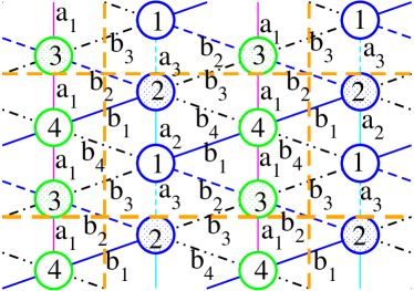
Graphene has a honeycomb lattice structure and it has two sites in the unit cell. There exists one electron per each site, i.e. the band is half-filled in graphene. On the other hand, -(BEDT-TTF)2I3 has four sites in the unit cell as shown in Fig. 1, where the small transfers between planes are neglected. The band made from the molecular orbits of BEDT-TTF molecules is 3/4 filled, since one electron is moved from two BEDT-TTF molecules to I3 molecule. The four sites in the unit cell make the Dirac points appear at and filled cases besides the half-filled case.
We study the filled band in -(BEDT-TTF)2I3 by using the tight-binding model in two dimension. The bulk properties of -(BEDT-TTF)2I3 can be expressed by the effective two-band model[11, 12, 13], which is similar to the model of the graphene with next-nearest hoppings[12, 14, 15]. However, when we consider the edge states, the effective two-band model cannot be applied.
In this paper, we study the edge states in -(BEDT-TTF)2I3 at 3/4 filling and compare these edge states with the edge states in graphene at half-filling. We show that the edge states always appear either in the region of or for the vertical edges and in the region of or for the horizontal edges, depending on the choice of the possible edges, where are are the wave number of the eigenstate and are the wave number of the two Dirac points in the bulk system.
2 Model
We study the tight-binding model for the quasi-two-dimensional conductor -(BEDT-TTF)2I3. There are four sites in the unit cell, which we label as sites , , , and , as shown in Fig. 1. There are the hoppings along the direction, , and , and the inter-chain hoppings . The system has the inversion symmetry[16, 17, 18]. The inversion center is located at the site , the site , and the center of the sites and . With the inversion the sites and are exchanged each other but the sites and remain unchanged. The sites , , and are also called AI, AII, B and C, or A, A′, B, and C, respectively. We also take account the site energies , , and . When , the inversion symmetry is conserved.[18] The energy of electrons in the tight binding approximation is given by the equation
| (2) | |||
| (3) | |||
| (4) | |||
| (5) |
where are the wave functions at sites in the unit cell with integers and . The parameters are estimated by Kondo et al.[19, 18] and used by Kobayashi et al.[20] as , , , , , and , where is the uniaxial strain in the direction. In this paper we use the parameter at kbar, i.e. , , , , , and .
3 Bulk system
If the system is infinite or periodic with respect to both and directions, the eigenstates are written as
| (6) |
Then the energy is obtained by
| (7) |
where
| (8) |
| (9) |
| (10) | ||||
| (11) | ||||
| (12) | ||||
| (13) |
If (i.e. ) and , the eigenvalues of the matrix in Eq. (9) are obtained by Mori[17] as
| (14) |
The condition for the Dirac points at the 1/4 and 3/4 filled band is obtained for this case of as,
| (15) |
This condition is fulfilled at , where and is given by
| (16) |
In order to have real solutions, the absolute value of the right hand side in Eq. (16) should be unity, from which we obtain
| (17) |
which has been obtained by Mori[17].
When and are not zero, which is the case in -(BEDT-TTF)2I3, the eigenvalues are complicated, although the analytical expression is possible as a solution of the quartic equation.
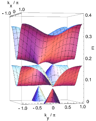
In Fig. 2, we show the 3D plot of the energy with the parameters for -(BEDT-TTF)2I3 with kbar and . In this figure we show the fourth and the third bands from the bottom of the energy (i.e. the first and the second band from the top of the energy) and the part of the second band from the bottom of the energy (the third band from the top of the energy). The first and the second bands from the top of the energy touch at two Dirac points . In this choice of parameters a finite gap exists between the second and the third bands as shown in Fig. 2. In this paper, however, we focus on the edge states in the three-quarter filled band and do not study the half-filled case, since we are interested in -(BEDT-TTF)2I3, which is the system with the 3/4-filled band.
4 Edge states
4.1 vertical edges
In this section we study the system with edges. The canted edges may be possible, but we consider the vertical and horizontal edges in this paper.
First we consider the vertical edges. We study two possibilities for each edge. The left edge and the right edge can be either the chain of the sites 1 and 2, or the chain of the sites 3 and 4 (see Fig. 1). Consider the ribbon of chains (where is integer) in which the left edge is the chain of sites and , and the right edge are the chain of the sites and . We call this system as the (12-34) edge. The other choices of the edges we will study for the vertical edges are the boundaries with the chain of the sites and at the left edge and the chain of the sites and at the right edge, which we call the (34-12) edge, the boundaries with chains of the sites and at both edges (the (12-12) edge), and the boundaries with chains of the sites and and at both edges, (the (34-34) edge). Note that the (34-12) edge has chains, while the (12-12) edge and the (34-34) edge have chains.
We assume the periodic boundary conditions in the direction for the systems with vertical edges, which means that we study the very long vertical ribbon or the tube similar to carbon nanotube.
Similar to the honeycomb lattice[10], we perform the Fourier transformation with respect to as
| (18) |
The energy and the eigenstate are obtained by the equation
| (19) |
where , , , are matrix given by
| (20) |
| (21) |
| (22) |
| (23) | ||||
| (24) | ||||
| (25) | ||||
| (26) | ||||
| (27) | ||||
| (28) |
and is the vector with wave functions,
| (29) |
In Eq. (19), we had introduced the parameter , which describe the boundary conditions. For the open boundary condition, in which the edge states may exist, we should take . The periodic boundary conditions can be obtained by taking .
In the same way we take the boundary with the 3 and 4 sites at the left edge and 1 and 2 sites at the right edge, which we call (34-12) edge. The energy of the (34-12) edge is the same as that of the (12-34) edge except that the left and the right edge states are exchanged.
In the (12-12) edge and the (34-34) edge, we cannot apply the periodic boundary conditions in the direction. The matrix size is in these edges.
Note that the (12-12) edge and the (34-34) edges are symmetric with respect to inversion, while the (12-34) edge and the (34-12) edge are not symmetric but they are exchanged each other by inversion.
4.2 horizontal edges
For the horizontal edges, the lower and upper boundaries have the zigzag shape. Each edge consists with one pair of the four possibilities, i.e., sites 4 and 2, 2 and 3, 3 and 1, or 1 and 4. There are 16 possibilities for the choice of the horizontal edges. We call these 16 possible edges as the (42-42) edge, the (42-23) edge, and so on. Considering that the sites 1 and 2 are exchanged each other by inversion while sites 3 and 4 are not changed by inversion, we obtain that the (42-14) edge, the (23-31) edge, the (31-23) edge and the (14-42) edge are symmetric with respect to inversion. The (31-42) edge, for example, becomes the (14-23) edge by inversion. For the horizontal edges, we can perform the Fourier transformation with respect to and the energy is labeled by .
There are eigenstates for each in the (42-31) edge, the (23-14) edge, the (31-42) edge and the (14-23) edge, where integer is the number of each sites () in each vertical chain. In these four cases we can apply the periodic boundary conditions with respect to direction, as in the cases of the (12-34) edge and the (34-12) edge for the vertical edges. If the periodic boundary conditions with respect to direction are taken, the above four cases give the same energy dispersion.
There are eigenstates for the (42-14) edge, the (23-42) edge, (31-23) edge and the (14-31) edge, where the lowermost and the uppermost sites are the same. When the lowermost and the second lower sites are the same as the second upper and the uppermost sites, such as the (42-42) edge, the (23-23) edge, the (31-31) edge and the (14-14) edge, there are eigenstates for each . When the second lower sites are the same as the second upper sites, such as the (42-23) edge, the (23-31) edge, the (31-14) edge and the (14-42) edge, there are eigenstates for each .
5 Results
(a)
(b)
(c)
(d)
(a)
(b)
(c)
(a)
(b)
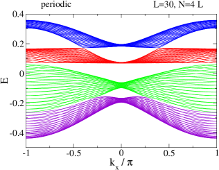
There are eigenstates and energies for each for the (12-34) edge and the (34-12) edge. We plot the energy as a function of in Fig. 3, where we use different colors for each band of states. There are edge states at the 1/4, 1/2 and 3/4 fillings of the band. In this paper we focus on the edge state at 3/4 filling case, since 3/4 filling is realized in -(BEDT-TTF)2I3.
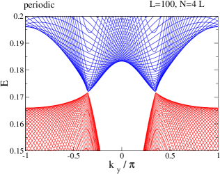
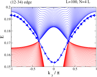
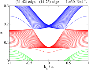
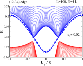
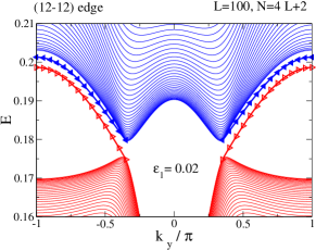
In Fig. 4 we plot the energies near the filling for the system with periodic boundary conditions for the x-direction, the (12-34) edge, the (12-12) edge and the (34-34) edge. If the system is periodic with respect to i.e., , we obtain the projection of the 3D plot of the energy (Fig. 2) as shown in Fig. 4(a).
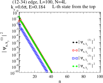
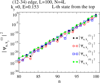
The eigenstates of the (12-34) edge at and for the -th state from the top and that at for the -th state are shown in Fig. 5 (a) , (b) and (c), respectively. The -th state from the top, i.e. the bottom of the highest band, is the edge state, which is localized at the left edge for (Fig. 5 (a)) and at the right edge for (Fig. 5 (b)). We define the localization length, , as
| (30) |
for the edge state localized at the left edge and
| (31) |
for the edge state localized at the right edge. It is obtained that at and at , as seen in Fig. 5(a) and (b). Other states such as the -th state, for example, are not the edge state as seen in Fig. 5(c).
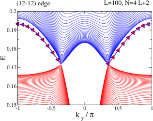
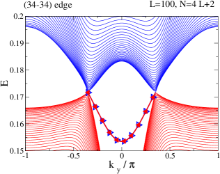
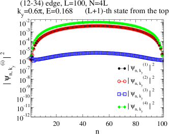
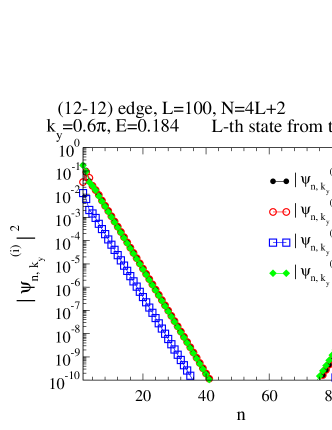
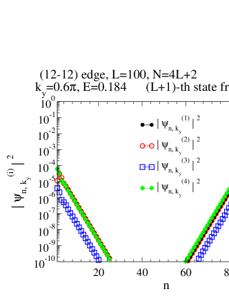
The edge states exist only at for the (12-12) edge and at for the (34-34) edge, as seen in Fig. 4 (c) and (d). In these cases the edge states are localized in both left and right edges. In general, when the localization length, , of the edge state is much smaller than the width (), the edge states at each edge can be treated as independent states, and these states degenerate due to inversion symmetry. Otherwise, the edge states at each edge interact each other and the degeneracy is lifted. Then the “bonding” and “anti-bonding” states of the each edge states become the eigenstates. In our numerical calculation for , which is much larger than the localization length, the -th and the -th states from the top have the same energy within the numerical accuracy and the eigenstates are any linear combinations of the left and the right eigenstates, as shown in Fig. 6, where -th and -th states are localized at both edges.
From the above results we conclude that if the left or right edge is the chain with sites 1 and 2, the edge states exists in the region near 3/4 filling. If the left or right edge is the chain with sites 3 and 4, the edge states exists in the region near 3/4 filling. We summarize the existence of the edge states in Table 1 (a).
| (a) vertical edge | |||
|---|---|---|---|
| left | edge state | right | edge state |
| 12 | 12 | ||
| 34 | 34 | ||
| (b) horizontal edge | |||
| lower | edge state | upper | edge state |
| 14 | 42 | ||
| 31 | 23 | ||
| 23 | 31 | ||
| 42 | 14 | ||
| vertical edge | |
|---|---|
| left, right | edge state |
| zigzag | |
| bearded (Klein’s edge[21]) | |
| horizontal edge | |
| lower, upper | edge state |
| armchair with Klein’s edge[22] | |
| armchair | |
(a)
(b)
(c)
(d)
(a)
(b)
(c)
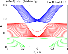
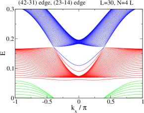
Next we study the horizontal edges. In Fig. 7 we plot the energy of the system with periodic boundary conditions as a function of . For various types of horizontal edges, we find that edge states always exist. We plot some examples of energy of the horizontal edges as a function of in Fig. 8.
We obtain that in the 3/4-filled case there are the edge states localized near the lower edge of the (14-xy) and (31-xy) edges when , where xy is either 14, 31, 23, or 42. Since (14-xy) and (31-xy) edges are changed to (y′x′-42) and (y′x′-23) edges by inversion, where y′x′ is either 42, 23, 31, or 14, respectively, (note that sites 1 and 2 are exchanged each other by inversion, while sites 3 and 4 are not changed.), there are edge states localized near the upper edge of (y′x′-42) and (y′x′-23) edges when .
We also obtain that there are the edge states localized near the lower edge of the (23-xy) and (42-xy) edges when , and there are the edge states localized near the upper edge of the (y′x′-31) and (y′x′-14) edges when . Table 1 (b) shows the summary of the existing region of the edge states for the horizontal edges.
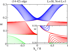
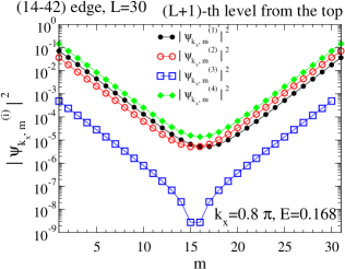
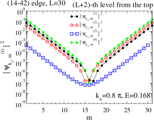
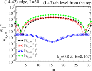
The edge states in the same rows in table 1 (b), for example, the lower 14 and upper 42, have the same energy dispersion. The edge states in different rows in table 1 (b), such as the lower 31 and upper 42, have different energies as a function of . In Fig. 8(a), we plot the energy as a function of the in the (31-42) edge (the (14-23) edge has the same energy). The -th and the -th states from the top of the energy are edge states at . The edge states in the -th state (at ) has a relatively large localization length and the energy of the edge state is close to the second band. The energy of the -th state at in the (31-42) edge (Fig. 8 (a)) is same as the -th state at in the (42-42) edge (Fig. 8 (b)) and the -the and the -th states in the (14-42) edge (Fig. 8 (c) and the inset). In Fig. 9 we plot the wave function of the -the, the -th and -th states in the (14-42) edge at as a function of the site number . It is clearly seen that the -th state and the -th state are the edge states localized at both lower and upper edges, while the -th state is not the edge state.
The energies as a function of for the edge states of the (23-xy) edge and the (42-xy) edge are different, as seen two curves between the first and the second bands (-th and (L+1)-th states) from the top of the energy at in Fig. 8 (d). As summarized in Table 1, all edges have the edge states at or for the vertical edge and at or for the horizontal edge.
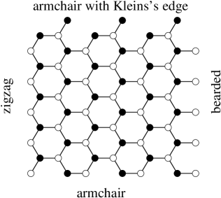
The edge states in -(BEDT-TTF)2I3 obtained above are compared to the edge states in graphene with anisotropic hoppings. In graphene there are two sites in the unit cell, forming A and B sublattices. These sites are exchanged by inversion. The edges in the graphene are classified as zigzag, bearded, zigzag-bearded and armchair[10]. We can also consider the armchair with the Klein’s edge[22]. These edges are shown in Fig. 10.
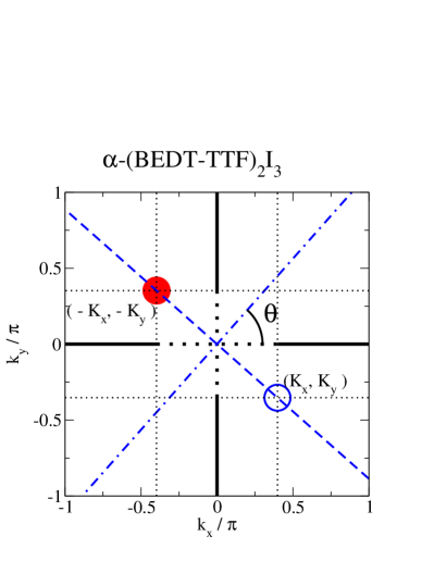
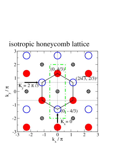
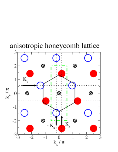
We consider the anisotropic cases with different hoppings between nearest neighbors in different directions[10]. For the isotropic honeycomb lattice the edge states exist in the zigzag, bearded and zigzag-bearded edges for , and any , respectively, while there is no edge states in the armchair edges. The Dirac points in the isotropic honeycomb lattice are located at , where is a lattice constant of the honeycomb lattice, as shown in Fig. 11(b). If we consider the anisotropic cases, however, it has been shown that the edge states exit even in the armchair edges[10]. The reason for the absence of the edge states in the isotropic honeycomb lattice with armchair edges can be understood as follows. In the armchair edges, the edge states can exist in the region where are the component of two Dirac points. In the case of the isotropic honeycomb lattice, the projections of the two Dirac points into axis coincide at . In that case there are no region of , which satisfies , and as a result there are no edge states in the isotropic armchair edges. On the other hand, if we consider the anisotropic honeycomb lattice with , we have the edge states at . Recently, it is also shown that the edge states exist in the isotropic honeycomb lattice with armchair edges moderated by the Klein’s defects[22]. In Table 2, the exiting region of the edge states are given.
We speculate that if we can make the tilted edges with the tilting angle , then coincidence of the projections of two Dirac points in the wave number along the tilted direction, as shown in Fig. 11(a). In that case we obtain the similar situation as in the isotropic honeycomb lattice with armchair edges and we expect that the edge states cannot exist.
(a)
(b)
(c)
One of the differences between the edge states in -(BEDT-TTF)2I3 and the edge states in graphene is that all four components of the wave functions decays exponentially away from the edge in edge states in -(BEDT-TTF)2I3, while one component of the wave function is always zero and the other component decays exponentially in the edge states in graphene. The other difference is the wave number dependence of the energy of the edge state. The energy of the edge states in -(BEDT-TTF)2I3 has strong or dependence, which is in contrast with the edge states in graphene, where the energy of the edge states is zero if the next-nearest-neighbor hoppings are not taken into account. The edge states in graphene have the dependent energy only when the next-nearest-neighbor hoppings are finite.[8, 9]
The energy dispersion of the edge states results in the occupation of the edge states at in (12-34) edge when the system is 3/4 filled, since the energy of the edge states is lower than the energy at the Dirac points, as seen in Fig. 4 (b). In that case only the edge states at the right edge are occupied. Similarly, the energy of the edge states for the horizontal edge have a wave-number dependence, as seen in Fig. 8.
6 Site energy
(a)
(b)
(a)
(b)
(a)
(b)
(c)
(a)
(b)
In this section we study the effect of the site energies . Note that and do not violate the inversion symmetry but and violate the inversion symmetry if . When , the dispersion of the eigenstates is only shifted by the constant energy. Therefore, if we consider the system with inversion symmetry, and are the relevant parameters. Either or can be taken as a parameter for the breaking of the inversion symmetry.
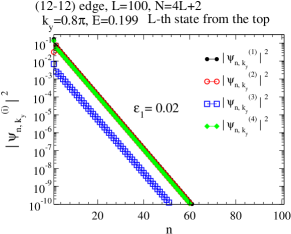
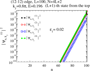
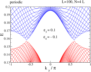
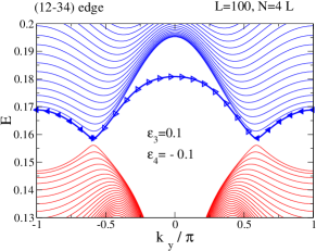
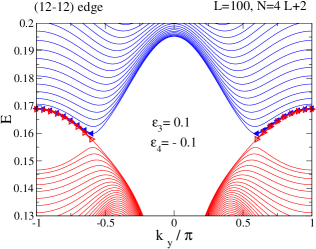
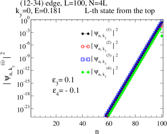
The energy gap is opened when inversion symmetry is broken by or , as shown in Fig. 12. Even if the gap is opened by or , the edge states still exist. As seen in Fig. 12 (a) the -th state from the top in the system with (12-34) edge is the left edge state for and the right edge state for , which is the same as in the system with inversion symmetry (see Fig. 4(b)). The (12-12) edge has the edge states for as shown in Fig. 12 (b). Because the inversion symmetry is broken, the left and right edge states are not degenerated. The -th state from the top of the energy is the edge state localized at the left edge, and the -th state is the edge state at the right edge. The localization length of these edge states are different as shown in Fig. 13 (a) and (b).
As seen in Fig. 12, the edge states with have the similar strong dependent energy as in the system with inversion symmetry. As a result, if the system is 3/4 filled, i.e. the chemical potential is in the middle of the gap of the bulk system (for example in Fig. 12 (a) and (b)), the localized state at the right edge is partially filled.
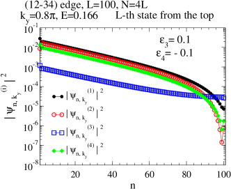
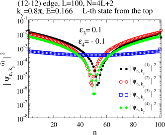
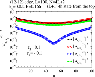
The first and the second bands from the top of the energy still touch each other at the Dirac points even when we take finite and (as an example we take and ), as shown in Fig. 14 (a) for the periodic boundary conditions. In that parameters ( and ), the edge states exist as in the case of (see Fig. 4 and Fig. 14). The localization length, however, differs from that in the case of . While the -th state from the top at in the (12-34) edge is the edge state localized at the right edge with the localization length (Fig. 15), the -th state at is the edge state at the left edge with the large localization length (Fig 16). The large localization length is more clearly seen in the (12-12) edge. The -th and -th states at are almost degenerate in energy in the system with . However the wave function of the -th state are different from that of the -th state as shown in Fig. 17. The square of the absolute values of the wave functions, , of -th and -th states from the top at are asymmetric and symmetric with respect to and they look like “anti-bonding” and “bonding” states, respectively. This means that these states are indeed the localized edge states but the system size () is not large enough for the edge states to be treated as independent states at each edges. In these cases the estimation of the localization length by Eqs. (30) or (31) may have an ambiguity and should be taken carefully. The localization lengths for should be same for all but depend on the component as we give the estimation in the figure captions. Even in these cases, the existing regions of the edge states are given in Table 1 with varied according to the choice of and .
7 Summary and discussions
In this paper we study the edge states in -(BEDT-TTF)2I3 in the absence of the magnetic field, theoretically. We have shown that the edge states exist in the 3/4 filled band in the system with four sites in the unit cell, such as -(BEDT-TTF)2I3. We study the vertical and horizontal edges. We show that all edges have the edge states as summarized in Table 1. In the edge states all components of the wave function decays exponentially as a function of the distance from the edge. Since the edge state has the wave-number dependent energy, it is possible to occupy only the left edge state or the lower edge states at 3/4 filling system. For example, in the (12-34) or (34-12) edges only the localized state at the right edge or the left edge is occupied in 3/4 filling system, respectively.
We also study the effect of the site energies, , , and . When the inversion symmetry is broken by or , a finite gap appears at the Dirac points. Even in that case the edge states exist as in the system with inversion symmetry. Due to the dependence of the edge states, the energy of the edge states can locate in the middle of the bulk band gap. Therefore, the insulator at the bulk sample has the partially filled edge states. These states are not the topologically protected edge states, which are recently predicted[23, 24, 25] and observed[26, 27, 28] in the topological insulators.
The opening of the gap at the Dirac points can be possible either by the breaking of the inversion symmetry (in the honeycomb lattice with next-nearest-neighbor hoppings the necessary symmetry for the zero gap is not the inversion symmetry but the “averaged inversion symmetry”.[14, 15]) or by the merging of the Dirac points.[29, 11, 30] If the inversion symmetry is not broken in (BEDT-TTF)2I3, the opening of the gap at the Dirac points occurs only when two Dirac points merge at modulo a reciprocal vector, i.e. , , or , which is predicted to occur at high pressure[11]. In the present choice of parameters, the finite gap at the half-filling as seen in Fig. 2 is caused by the merging of the Dirac points at . The edge states also exist even when the gap is opened either by the breaking of the inversion symmetry or the merging of the Dirac points.
With finite and the gap remains zero at the Dirac points, but the localization lengths of the edge states may be changed drastically. The edge states with the large localization length can be realized if we can tune the site energies.
The experimental observation of the edge states in -(BEDT-TTF)2I3 will be possible and provide us more insight about the massless Dirac particles realized in the quasi-two-dimensional conductors.
References
- [1] N. Tajima, S. Sugawara, M. Tamura, Y. Nishino and K. Kajita, J. Phys. Soc. Jpn. 75 (2006) 051010.
- [2] S. Katayama, A. Kobayashi and Y. Suzumura, J. Phys. Cos. Jpn. 75 (2006) 054705.
- [3] T. Osada, J. Phys. Soc. Jpn. 77 (2008) 084711.
- [4] N. Tajima, S Sugawara, R. Kato, Y. Nishio, and K. Kajita, Phys. Rev. Lett. 102 (2009)176403.
- [5] K. S. Novoselov, A. K. Geim, S. V. Morozov, D. Jiang, M. I. Katsnelson, I. V. Grigorieva, S. V. Dubonos and A. A. Firsov, Nature (London) 438 (2005) 197.
- [6] Y. Zhang, Y. W. Tan, H. L. Stormer, and P. Kim, Nature (London) 438 (2005) 201.
- [7] M. Fujita, K. Wakabayashi, K. Nakada, K. Kusakabe, J. Phys. Soc. Jpn. 65 (1996) 1920.
- [8] K. Sasaki, S. Murakami, and R. Saito, Appl. Phys. Lett. 88 (2006) 113110.
- [9] N. M. R. Peres, F. Guinea, and A. H. Castro Neto, Phys. Rev. B 73 (2006) 125411.
- [10] M. Kohmoto and Y. Hasegawa, Phys. Rev. B 76 (2007) 205402.
- [11] A. Kobayashi, S. Katayama, Y. Suzumura and H. Fukuyama, J. Phys. Soc. Jpn. 76 (2007) 034711.
- [12] M.O. Georbig, J.N. Fuchs, G. Montambaux and F. Piechon, Phys. Rev. B 78 (2008) 045415.
- [13] T. Morinari, T. Himura and T. Tohyama, J. Phys. Soc. Jpn. 78 (2009) 023704.
- [14] K. Kishigi, H. Hanada, and Y. Hasegawa, J. Phys. Soc. Jpn. 77 (2008) 074707.
- [15] K. Kishigi, R. Takeda and Y. Hasegawa, J. Phys., Conf. Ser. 132 (2008) 012005.
- [16] T. Mori, A. Kobayashi, Y. Sasaki, H. Kobayashi, G. Saito, and H. Inokuchi, Chem. Lett. 13 (1984) 957.
- [17] T. Mori, J. Phys. Soc. Jpn. 79 (2010) 014703.
- [18] R. Kondo, S. Kagoshima, N. Tajima and R. Kato, J. Phys. Soc. Jpn. 78 (2009) 114714.
- [19] R. Kondo, S. Kagoshima, and J. Harada, Rev. Sci. Instrum. 76 (2005) 093902.
- [20] A. Kobayashi, Y. Suzumura, H. Fukuyama and M. O. Goerbig, J. Phys. Soc. Jpn. 78 (2009) 114711.
- [21] D.J. Klein, Chem Phys. Lett. 217 (1994) 261.
- [22] K. Wakabayashi, S. Okada, R. Tomita, S. Fujimoto, and Y. Natsume, J. Phys. Soc. Jpn. 79 (2010) 034706.
- [23] C. L. Kane and E. J. Mele, Phys. Rev. Lett. 95 (2005) 226801.
- [24] B. A. Bernevig, T. L. Hughes, S. C. Zhang Science, 314 (2006) 1757.
- [25] L. Fu, C. L. Kane and E. J. Mele, Phys. Rev. Lett. 98 (2007) 106803.
- [26] M. König, S. Wiedmann, C. Brune, A. Roth, H. Buhmann, L. W. Molenkamp, X. L. Qi, S. C. Zhang, Science 318 (2007) 766.
- [27] D. Hsieh, D. Qian, L. Wray, Y. Xia, Y. S. Hor, R. J. Cava and M. Z. Hasan1, Nature 452 (2008) 970.
- [28] M. König, H. Buhmann, L. W. Molenkamp, T. Hughes, C. X. Liu, X. L. Qi, and S. C. Zhang J. Phys. Soc. Jpn. 77 (2008) 031007.
- [29] Y. Hasegawa, R. Konno, H. Nakano, and M. Kohmoto, Phys. Rev. B 74 (2006) 033413.
- [30] G. Montambaux, F. Piechon, J.N. Fuchs, and M.O. Georbig, Phys. Rev. B 80 (2009) 153412.