Dynamical Lorentz symmetry breaking and topological defects

Abstract

I discuss the possibility of topological defect solutions in field theories containing a tensor field which spontaneously breaks Lorentz symmetry. I find that for theories of a tensor with rank $r\leq 5$ and for which the vacuum manifold consists of the tensors whose “square” is some constant value, only three types of tensor (vectors, antisymmetric two-tensors, and symmetric two-tensors) have the appropriate vacuum manifold topology to support topological defects. Of these, topological defect solutions can be easily constructed for two: vector domain wall solutions and antisymmetric tensor monopole solutions. These antisymmetric tensor monopole solutions are in principle detectible via their gravitational lensing effects.

I Introduction

The idea of Lorentz symmetry violation has been a subject of sustained research activity for some years now. In such theories, one typically postulates the existence of a non-zero tensor on spacetime that couples to “conventional” matter such as electrons, quarks, photons, and so forth. The so-called “Standard Model Extension”, or SME Colladay and Kostelecký (1998), provides a wide-ranging framework within which to analyse the physical effects of such symmetry violations. While no unambiguous evidence for such fields has yet been found, many experimental bounds on their effects have been obtained Kostelecký and Russell (2010), and research is ongoing.

It is, of course, natural to ask what the origin of this “Lorentz-violating” tensor might be. It is known that the fiat specification of a fixed background tensor field, while acceptable in a flat spacetime, is in general not mathematically consistent with making the metric dynamical Kostelecký (2004). However, a self-consistent theory can be obtained by allowing the Lorentz-violating field to itself be dynamical. In this scenario, the tensor field is usually taken to have a potential energy that is minimized (and vanishes) when the tensor takes on a non-zero value; this non-zero value can be said to spontaneously break the Lorentz symmetry of the underlying Lagrangian. This scenario closely parallels the behaviour of the Higgs field in the Standard Model; however, in our case the field taking on a background expectation value is a spacetime tensor rather than a spacetime scalar. The usual “particle physics” portion of the SME, with conventional matter fields coupling to a constant background tensor in flat spacetime, can be obtained as an effective field theory limit with the dynamics of the Lorentz-violating tensor field integrated out.

While this picture is self-consistent and fairly compelling, it also raises an interesting corollary possibility. In general, a field which spontaneously breaks some symmetry in vacuo will, at sufficiently high temperatures, see that symmetry restored. This implies that in the early Universe, a Lorentz-violating tensor field will have zero expectation value; as the Universe expands and cools, we would eventually expect this field to undergo a phase transition from a state of higher symmetry (a vanishing tensor field) to a state of lower symmetry (a non-vanishing tensor field.)

A field whose Lagrangian possesses some symmetry but whose solutions break that symmetry will generally not have a unique minimum to its potential; this space of all possible vacuum values is known as the vacuum manifold. Since there is more than one possible vacuum value for the field, it is likely that causally disconnected portions of the Universe would “choose” different values of the field in the symmetry-breaking phase transition. Moreover, if this manifold has particular topological properties, regions that “fall into” different portions of the vacuum manifold will be unable to evolve to match up with one another without a significant energy input. Such field configurations are known as topological defects, and the idea that such configurations might arise in the natural evolution of the Universe was first put forward by Kibble Kibble (1976). The existence of such solutions relies crucially on the topology of the vacuum manifold; an arbitrary field theory will not, in general, allow for topological defect solutions.

In the present work, I will address the question of whether topological defect solutions can arise in theories with a tensor field that spontaneously breaks Lorentz symmetry. After some preliminaries (Section II), I discuss the topology of vacuum manifolds of tensor fields in Section III. In Section IV, I find maximally symmetric topological defect solutions for those tensor fields that can support them; their basic physical properties are described in Section V. Finally, I discuss more general issues arising from this work in Section VI.

Throughout this work, we will use units in which $\hbar=c=1$; sign conventions for the metric and curvature will be those of Wald Wald (1984). In particular, the metric signature will be $(-,+,+,+)$.

II Preliminaries

Most theories of current interest in which Lorentz symmetry is spontaneously violated follow from an action of the form

$$S=\int\mathrm{d}^{4}x\left(\frac{1}{2}\mathcal{T}\cdot\mathcal{O}[\mathcal{T}]-V(\mathcal{T})\right),$$ (1)

where $\mathcal{T}$ is a tensor field of some rank $r$, potentially with some symmetry relations; $\mathcal{O}$ is a linear, second-order, self-adjoint, strictly differential operator on tensors of rank $r$; and $V(\mathcal{T})$ is the potential energy for $\mathcal{T}$. (We assume for the moment a fixed flat background.) The equation of motion derived from an action of this form is then

$$\mathcal{O}[\mathcal{T}]-\frac{\delta V(\mathcal{T})}{\delta\mathcal{T}}=0.$$ (2)

The potential term $V$ is a Lorentz scalar. Assuming that we do not have any background geometric structure in this theory, this means that $V$ must be a function of the various scalars that can be formed out of $\mathcal{T}$ via contraction of its indices with the metric $\eta_{ab}$. For example, if $\mathcal{T}$ is an arbitrary two-index tensor $t_{ab}$, we could have

$$V(t_{ab})=V(t_{a}{}^{a},t_{ab}t^{ab},t_{ab}t^{ba},t_{a}{}^{b}t_{b}{}^{c}t_{c}{}^{a},\dots).$$ (3)

For the purposes of this paper, we will only consider potential terms of the form

$$V(\mathcal{T})=V(\mathcal{T}^{a_{1}a_{2}\cdots a_{r}}\mathcal{T}_{a_{1}a_{2}\dots a_{r}})\equiv V(\mathcal{T}^{(a_{i})}\mathcal{T}_{(a_{i})}),$$ (4)

where we have introduced the notation $(a_{i})$ to represent the index string $a_{1}a_{2}\cdots a_{r}$. (Where there is no risk of confusion, we will use $(a)$ the same way.) For a potential of this form, the potential term in the equation of motion will just be

$$\frac{\delta V(\mathcal{T}^{(a)})}{\delta\mathcal{T}^{(a)}}=2V^{\prime}(\mathcal{T}^{(a)}\mathcal{T}_{(a)})\mathcal{T}_{(a)}.$$ (5)

This equation implies that if $\mathcal{T}^{(a)}$ takes on a constant value $\bar{\mathcal{T}}^{(a)}$ everywhere in spacetime, such that $V^{\prime}(\bar{\mathcal{T}}^{(a)}\bar{\mathcal{T}}_{(a)})=0$, then the equation of motion (2) will be satisfied. If the potential $V$ is constructed in such a way that it is minimized at a non-zero value of its argument, then $\mathcal{T}^{(a)}$ will be non-zero in this solution.

In this way, this model will spontaneously break Lorentz symmetry. The above mentioned solutions of the equations of motion will not be Lorentz-invariant: they contain a non-zero tensor field $\mathcal{T}_{(a)}=\bar{\mathcal{T}}_{(a)}$ throughout spacetime, which imparts a preferred geometric structure to flat spacetime. Couplings between our Lorentz-violating field and “conventional” matter fields (akin to the hypothesized Yukawa coupling between fermion fields and the Higgs field) could then give rise to a wide variety of observable physical phenomena Kostelecký and Russell (2010).

It is important to note, however, that the specific value of $\bar{\mathcal{T}}^{(a)}$ is not uniquely determined by the equations of motion; in fact, the action (1) is completely Lorentz-invariant. Rather, any constant tensor field satisfying $\mathcal{T}^{(a)}\mathcal{T}_{(a)}=C$, where $V^{\prime}(C)=0$, will be a solution of the equations of motion. The set of all such tensors will form a submanifold $M_{\text{vac}}$ in the space $\mathbb{V}$ of tensors under consideration. The shape of this manifold will be critical in determining whether a tensor field taking values in $\mathbb{V}$ can give rise to topological defects; it is to this question that we now turn.

III Vacuum Manifolds

The idea of topological defects in field theories is not a new one; a thorough description of the idea in the context of high-energy physics can be found in Vilenkin and Shellard (1994), to which the interested reader is referred. For the purposes of this work, a topological defect can be thought of as a solution of the equations of motion for which the fields asymptotically approach a minimum-energy value as we go to spatial infinity, but for which this minimum-energy value is dependent on the direction that we go to infinity. The types of topological defects that can arise as solutions of a given theory will depend critically on the topology of that theory’s vacuum manifold $M_{\text{vac}}$. If the vacuum manifold is disconnected, we can have domain wall solutions; if the vacuum manifold contains non-contractible loops, cosmic strings may arise; and if the vacuum manifold contains non-contractible two-spheres, we can potentially have monopole solutions. In terms of the homotopy groups of the manifold, such structures will arise if the groups $\pi_{0}(M_{\text{vac}})$, $\pi_{1}(M_{\text{vac}})$, or $\pi_{2}(M_{\text{vac}})$ (respectively) are non-trivial.

To identify what types of topological defects can arise in our theory, then, we need to know the topology of our vacuum manifold. As noted above, we will be concerned in this paper with the set of all tensors $\mathcal{T}^{(a)}\in\mathbb{V}$ with a fixed “tensor norm” given by

$$\eta_{(a)(b)}\mathcal{T}^{(a)}\mathcal{T}^{(b)}=C,$$ (6)

where we have defined

$$\eta_{(a)(b)}=\eta_{a_{1}b_{1}}\eta_{a_{2}b_{2}}\cdots\eta_{a_{r}b_{r}}.$$ (7)

$\mathbb{V}$ here is the space of all tensor of a definite rank and symmetry type; since such sets are closed under addition and scalar multiplication, we can view $\mathbb{V}$ as a real vector space. The tensor norm (6) defines a quadratic form (not necessarily definite) on $\mathbb{V}$. In the Appendix it is shown that this quadratic form is non-degenerate for tensors of definite rank and symmetry type non-degenerate. This implies that we can pick an orthonormal basis for $\mathbb{V}$, i.e., a set of $n$ tensors $\{(e_{i})^{(a)}\}\in\mathbb{V}$ such that

$$\eta_{(a)(b)}(e_{i})^{(a)}(e_{j})^{(b)}=\pm\delta_{ij},$$ (8)

where $i$ and $j$ take on the values $\{1,\dots,n\}$, the plus sign holds for the first $n_{+}$ of the basis elements, and the minus sign holds for the remaining $n_{-}$. In other words, $\mathbb{V}$ is an $n$-dimensional real vector space on which we have a metric $\eta_{(a)(b)}$ of signature $(n_{+},n_{-})$. As the tensors $\{(e_{i})^{(a)}\}$ form a basis for $\mathbb{V}$, we can decompose an arbitrary tensor $\mathcal{T}^{(a)}$ in terms of components with respect to this basis:

$$\mathcal{T}^{(a)}=\sum_{i=1}^{n}\mathcal{T}_{i}\,(e_{i})^{(a)}.$$ (9)

We can then use the orthogonality properties (8) of our basis to write the tensor norm (6) in terms of these components:

$$\eta_{(a)(b)}\mathcal{T}^{(a)}\mathcal{T}^{(b)}=\mathcal{T}_{1}^{2}+\mathcal{T}_{2}^{2}+\dots+\mathcal{T}_{n_{+}}^{2}-\mathcal{T}_{n_{+}+1}^{2}-\dots-\mathcal{T}_{n}^{2}.$$ (10)

Our vacuum manifold $M_{\text{vac}}$ will thus be the set of all tensors for which this norm is a given constant $C$. It is not hard to see that $\mathbb{V}$ is equivalent to $\mathbb{R}^{n}$ (since the $\mathcal{T}_{i}$’s can be viewed as coordinates on $\mathbb{V}$), and that $M_{\text{vac}}$ will be some $(n-1)$-dimensional hyperboloid embedded in $\mathbb{R}_{n}$. Specifically, we note that if $C>0$, our vacuum manifold will be the space of all tensors whose components satisfy

$$\mathcal{T}_{1}^{2}+\dots+\mathcal{T}_{n_{+}}^{2}=\mathcal{T}_{n_{+}+1}^{2}+\dots+\mathcal{T}_{n}^{2}+C.$$ (11)

This hyperboloid can be seen to be topologically equivalent to $S^{n_{+}-1}\times\mathbb{R}^{n_{-}}$: for any value of the $n_{-}$ components $\mathcal{T}_{n_{+}+1}$ through $\mathcal{T}_{n}$, the components $\mathcal{T}_{1}$ through $\mathcal{T}_{n_{+}}$ are constrained to lie on an $(n_{+}-1)$-sphere whose radius squared is the right-hand side of (11). Similarly, for $C<0$, we can rearrange (10) to yield

$$\mathcal{T}_{n_{+}+1}^{2}+\dots+\mathcal{T}_{n}^{2}=\mathcal{T}_{1}^{2}+\dots+\mathcal{T}_{n_{+}}^{2}+(-C),$$ (12)

which, by similar logic, yields a space that is topologically equivalent to $S^{n_{-}-1}\times\mathbb{R}^{n_{+}}$. Thus, in both cases the vacuum manifold is homeomorphic to $S^{p}\times\mathbb{R}^{q}$ for some $p$ and $q$.

We can now see that the topology of $M_{\text{vac}}$, and thus the possibility of topological defects in theories with spontaneous Lorentz breaking, depends heavily on the signature of the metric $\eta_{(a)(b)}$ induced on $\mathbb{V}$. Since $\mathbb{R}^{q}$ is a contractible space for all $q$, it follows that $\pi_{N}(S^{p}\times\mathbb{R}^{q})=\pi_{N}(S^{p})$ for all $N$. Moreover, since we are interested in topological defects, we only need to consider the lower-dimensional homotopy groups $\pi_{0}$, $\pi_{1}$, and $\pi_{2}$; for a $p$-sphere, these groups are non-trivial if and only if $p=0$, 1, or 2 respectively. Thus, the lower-dimensional homotopy groups of our vacuum manifold $M_{\text{vac}}$ will be trivial unless either $n_{+}$ or $n_{-}$ is less than or equal to 3; if both are greater than 3, localized topological defects cannot arise.

Rank &		$(n_{+},n_{-})$
symmetry type		General	Trace-free
$r=0$	$\emptyset$	$(1,0)$	$(1,0)$
$r=1$	$\yng(1)$	$(3,1)$	$(3,1)$
$r=2$	$\yng(2)$	$(7,3)$	$(6,3)$
	$\yng(1,1)$	$(3,3)$	$(3,3)$
$r=3$	$\yng(3)$	$(13,7)$	$(10,6)$
	$\yng(2,1)$	$(11,9)$	$(8,8)$
	$\yng(1,1,1)$	$(1,3)$	$(1,3)$
$r=4$	$\yng(4)$	$(22,13)$	$(15,10)$
	$\yng(3,1)$	$(24,21)$	$(15,15)$
	$\yng(2,2)$	$(12,8)$	$(5,5)$
	$\yng(2,1,1)$	$(6,9)$	$(3,6)$
	$\yng(1,1,1,1)$	$(0,1)$	$(0,1)$
$r=5$	$\yng(5)$	$(34,22)$	$(21,15)$
	$\yng(4,1)$	$(45,39)$	$(24,24)$
	$\yng(3,2)$	$(33,27)$	$(12,12)$
	$\yng(3,1,1)$	$(15,21)$	$(6,10)$
	$\yng(2,2,1)$	$(11,9)$	$(0,0)$
	$\yng(2,1,1,1)$	$(1,3)$	$(0,0)$

Table 1: Signatures of the spaces of tensors of definite symmetry type with rank $r\leq 5$, with and without traces subtracted, in $d=4$.

We have thus reduced the problem of determining the topology of the vacuum manifold of a Lorentz-breaking tensor field to that of determining the signature of the space $\mathbb{V}$ in which it lies. These signatures can be determined by the iterative procedures described in the Appendix; the results, for both general and trace-free tensors of rank $r\leq 5$ and definite symmetry type (labelled by Young tableaux), are given in Table 1. We note that only three types of tensors (not counting the scalar) have the correct vacuum topology to support topological defects in three spatial dimensions:

• Vectors ($r=1$). The space of vectors $v^{a}$ for which $v^{a}v_{a}=C$, with $C<0$, has topology $S^{0}\times\mathbb{R}^{3}$. Note that $S^{0}$ is a set containing two discrete points; the vacuum manifold is thus the topologically equivalent to two disconnected copies of $\mathbb{R}^{3}$, which can be seen to be the past-oriented and future-oriented timelike vectors of a given norm. Alternately, the space of vectors for which $v^{a}v_{a}=C>0$ has topology $S^{2}\times\mathbb{R}$. In principle, then, vectors that spontaneously break Lorentz symmetry could give rise to either domain wall or monopole solutions, depending on whether the vacuum manifold consists of timelike or spacelike vectors respectively.

• Antisymmetric two-tensors. The space of such tensors $B^{ab}$ for which $B^{ab}B_{ab}=C$ will have topology $S^{2}\times\mathbb{R}^{3}$ for any non-vanishing $C$ (positive or negative.) Thus, these tensors could in principle give rise to monopoles.

• Symmetric two-tensors, with or without trace. The space of such tensors $h^{ab}$ for which $h^{ab}h_{ab}=C<0$ will have topology $S^{2}\times\mathbb{R}^{7}$ (or $S^{2}\times\mathbb{R}^{6}$ for trace-free tensors.) Such tensors could then in principle give rise to monopoles as well.

The remaining tensors in Table 1 with low signatures (i.e. $n_{+}\leq 3$ or $n_{-}\leq 3$) can be shown to be equivalent to either the scalar or one of the three types of tensors above; see the Appendix and Hamermesh (1962) for details.

IV Existence of topological defect solutions

In the previous section, we found that the vacuum manifolds $\mathcal{T}^{(a)}\mathcal{T}_{(a)}=C$ of only three types of tensors (vectors, antisymmetric two-tensors, and symmetric two-tensors) have the appropriate topology to support topological defects. All other tensors with rank $r\leq 5$ either have both $n_{+}$ and $n_{-}$ too large to support topological defects in three spatial dimensions, or are equivalent to one of these three types of tensors.

While the existence of a vacuum manifold of the proper topology is a necessary condition for the existence of topological defect solutions, it is not a sufficient condition. By a topological defect solution, we mean a solution of the equation of motion

$$\mathcal{O}_{(a)}[\mathcal{T}]-2V^{\prime}(\mathcal{T}^{(b)}\mathcal{T}_{(b)})\mathcal{T}_{(a)}=0$$ (13)

such that the tensor field $\mathcal{T}^{(a)}$ goes asymptotically to its vacuum manifold, and such that the asymptotic map between “spatial infinity” (in the appropriate sense) and the vacuum manifold is topologically non-trivial. While such asymptotic maps are easily constructed, the global existence of such solutions will also depend on the properties of the kinetic operator $\mathcal{O}$. (See Babichev (2006) for an example of this in the scalar case.) We must thus ask what type of operators are appropriate for our theories.

Fortunately, for the three types of tensor fields under consideration, there are already “natural” choices of kinetic term. For the vector and anti-symmetric two-tensor cases, we can choose a “field strength–squared” kinetic term. Specifically, for the vector field $A^{a}$, we can write

$$S_{A}=\int\mathrm{d}^{4}x\left(-\frac{1}{4}F^{ab}F_{ab}-V(A^{a}A_{a})\right),$$ (14)

where $F_{ab}=2\partial_{[a}A_{b]}$. For the antisymmetric two-tensor $B_{ab}$, we can write

$$S_{B}=\int\mathrm{d}^{4}x\left(-\frac{1}{6}F^{abc}F_{abc}-V(B^{ab}B_{ab})\right),$$ (15)

where $F_{abc}=3\partial_{[a}B_{bc]}$. (A recent study of this and related models can be found in Altschul et al. (2010).) For the symmetric two-tensor, meanwhile, we can take the standard kinetic operator $\mathcal{K}$ for a massless spin-2 field:

$$S_{\gamma}=\int\mathrm{d}^{4}x\left(\frac{1}{2}\gamma^{ab}\mathcal{K}_{abcd}\gamma^{cd}-V(\gamma^{ab}\gamma_{ab})\right)$$ (16)

where

$$\mathcal{K}_{abcd}=\frac{1}{2}\left[(\eta_{a(c}\eta_{d)b}-\eta_{ab}\eta_{cd})\Box+\eta_{ab}\partial_{c}\partial_{d}\right.\\ \left.+\eta_{cd}\partial_{a}\partial_{b}-\eta_{a(c}\partial_{d)}\partial_{b}-\eta_{b(c}\partial_{d)}\partial_{a}\right].$$ (17)

The exact field profile of any topological defect solutions will also depend on the form of the tensor potential $V(x)$. However, the existence of such solutions is in general largely independent of the exact functional form of $V(x)$; as long as $V(x)$ has a single minimum at a value of $x$ of the appropriate sign, any other changes to $V(x)$ will just change the fine details of the field profile of the defect solution. For concreteness, we will take $V(x)$ to in all three cases be of the form

$$V(x^{2})=\frac{\lambda}{2}(x^{2}\pm b^{2})^{2},$$ (18)

where the sign is chosen depending on whether we want the topological defect to arise from the negative-norm components of our tensor or the positive-norm components. Note that in the case of a scalar field, this reduces to the familiar fourth-order double-well potential.

We are now in a position to look for topological defect solutions for tensor fields of the three types above. We will treat these cases below, in order of increasing physical interest.

IV.1 Symmetric tensors

In the case of symmetric two-tensors, we have $(n_{+},n_{-})=(7,3)$ (or $(6,3)$ if we require the trace to vanish.) Since $n_{+}>3$ and $n_{-}=3$, a topological defect solution (if it exists) will be a monopole, and the vacuum manifold will be of the form $\gamma^{ab}\gamma_{ab}=-b^{2}$. The Euler-Lagrange equation derived from the action (16) is

$$\mathcal{E}_{ab}\equiv\mathcal{K}_{ab}{}^{cd}\gamma_{cd}-2\lambda(\gamma_{cd}\gamma^{cd}+b^{2})\gamma_{ab}=0$$ (19)

The simplest possible topological defect solution will be one possessing spherical symmetry. This constricts the form that $\gamma_{ab}$ can take; the spherical coordinate components $\gamma_{\mu\nu}$ must be of the form

$$\gamma_{tt} =f(r), \gamma_{rt} =\gamma_{tr}=h(r),$$ (20)

$$\gamma_{rr} =g(r), \gamma_{\theta\theta} =\sin^{-2}\theta\gamma_{\phi\phi}=r^{2}i(r).$$ (21)

In terms of these functions, the independent coordinate components $\mathcal{E}_{\mu\nu}$ of the equations of motion are then

$$\mathcal{E}_{tt}=i^{\prime\prime}+\frac{3}{r}i^{\prime}+\frac{1}{r^{2}}i-\frac{1}{r}g^{\prime}-\frac{1}{r^{2}}g+2\lambda(\gamma^{2}+b^{2})f=0,$$ (22a)

$$\mathcal{E}_{tr}=2\lambda(\gamma^{2}+b^{2})h=0,$$ (22b)

$$\mathcal{E}_{rr}=\frac{1}{r}f^{\prime}+\frac{1}{r^{2}}g-\frac{1}{r}i^{\prime}-\frac{1}{r^{2}}i+2\lambda(\gamma^{2}+b^{2})g=0,$$ (22c)

and

$$\frac{1}{r^{2}}\mathcal{E}_{\theta\theta}=\frac{1}{2}\left(i^{\prime\prime}-\frac{2}{r}i^{\prime}+f^{\prime\prime}+\frac{1}{r}f^{\prime}+\frac{1}{r}g^{\prime}\right)\\ +2\lambda(\gamma^{2}+b^{2})i=0,$$ (22d)

where $\gamma^{2}\equiv f^{2}+g^{2}+2i^{2}-2h^{2}$ and primes denote derivatives with respect to $r$. It is evident from equation (22b) that we must either have $\gamma^{2}+b^{2}=0$ everywhere in spacetime—in which case our field is everywhere confined to the vacuum manifold—or we must have $h=0$ everywhere, in which case the field cannot asymptotically approach the vacuum manifold. Thus, we conclude that the symmetric two-tensor action (16) cannot support spherically symmetric topological defect solutions.

IV.2 Vectors

In the case of vector fields, we have $(n_{+},n_{-})=(3,1)$; thus, we could either have monopole solutions (if $C=b^{2}$) or domain wall solutions (if $C=-b^{2}$.) The Euler-Lagrange equation derived from the action (14) is

$$\mathcal{E}_{a}\equiv\partial^{b}F_{ba}-2\lambda(A_{b}A^{b}\pm b^{2})A_{a}=0.$$ (23)

Since the expected symmetry of the simplest topological defect solutions is different for spacelike and timelike vectors (spherical and planar, respectively), we must treat these cases separately.

IV.2.1 Spacelike vacuum manifold

If the vacuum manifold consists of all vectors $A^{a}$ with $A^{a}A_{a}=b^{2}$, our topological defect solution (if it exists) will be a monopole solution; thus, we look for solutions with spherical symmetry. The most general vector field with such a symmetry will be

$$(A^{t},A^{r},A^{\theta},A^{\phi})=(f(r),g(r),0,0).$$ (24)

This implies that the field strength tensor $F_{ab}$ has components $F_{tr}=-F_{rt}=f^{\prime}$, with all other components vanishing; the components of the equation of motion then become

$$\mathcal{E}_{t}=-f^{\prime\prime}-\frac{2}{r}f^{\prime}+2\lambda(-f^{2}+g^{2}-b^{2})f=0$$ (25a)

and

$$\mathcal{E}_{r}=-2\lambda(-f^{2}+g^{2}-b^{2})g=0.$$ (25b)

(Primes again denote differentiation with respect to $r$.) We see from equation (25b) that as in the symmetric tensor case, the field must either be in the vacuum manifold everywhere in spacetime or $g$ must vanish everywhere; neither case can correspond to a topological defect.

IV.2.2 Timelike vacuum manifold

The case where the vacuum manifold consists of all vectors $A^{a}$ with $A^{a}A_{a}=-b^{2}$ is somewhat more promising. In this case, we have the possibility of domain wall solutions. The simplest possible domain wall will have planar symmetry, with all fields depending on some Cartesian coordinate $x$; the vector field will take on the form

$$(A^{t},A^{x},A^{y},A^{z})=(f(x),g(x),0,0).$$ (26)

Using primes here to denote differentiation with respect to $x$, we have $F_{tx}=-F_{xt}=f^{\prime}$; the non-trivial components of the equation of motion (23) are

$$\mathcal{E}_{t}=-f^{\prime\prime}+2\lambda(-f^{2}+g^{2}+b^{2})f=0$$ (27a)

and

$$\mathcal{E}_{x}=-2\lambda(-f^{2}+g^{2}+b^{2})g=0$$ (27b)

As in the spacelike vector case, we see from (27b) that if we do not want the solution to lie in the vacuum manifold everywhere, the spacelike component of $A^{a}$ (namely $g$) must vanish. However, in this case the vanishing of $g$ is not an impediment to the field asymptotically approaching the vacuum manifold. In fact, the equation (27a) can be seen to be exactly that of the prototypical domain wall solution, arising in a theory of a single scalar field with a broken $\mathbb{Z}_{2}$ symmetry (see, for example, Chapter 3 of Vilenkin and Shellard (1994)). Its solution is

$$f(x)=\pm b\tanh\left(\sqrt{-\lambda}bx\right).$$ (28)

In this case, we find that a “Lorentz-violating” topological defect solution does exist; it is a domain wall configuration, with the vector field past-oriented on one side of the wall, future-oriented on the other, and smoothly interpolating through $A^{a}=0$ in between. Notably, if this solution is to exist, we must have $\lambda<0$; this will turn out to be quite important when we analyse the properties of this solution in Section V.1.

IV.3 Antisymmetric tensors

In the case of antisymmetric two-tensors, we have $(n_{+},n_{-})=(3,3)$. This implies that monopole solutions are topologically allowed for both positive-norm and negative-norm tensors. Since we expect both types of tensors to have spherically symmetric solutions, we can treat both cases simultaneously. The Euler-Lagrange equation derived from the action (15) is

$$\mathcal{E}_{ab}\equiv\partial^{c}F_{cab}-2\lambda(B^{cd}B_{cd}\pm b^{2})B_{ab}=0.$$ (29)

The most general antisymmetric two-tensor with spherical symmetry can be written in the form

$$B_{tr}=-B_{rt} =f(r), B_{\theta\phi}=-B_{\phi\theta} =g(r)r^{2}\sin\theta,$$ (30)

with all other components vanishing. There are then two non-trivial components of the equation of motion:

$$\mathcal{E}_{tr}=-2\lambda(-2f^{2}+2g^{2}\pm b^{2})f=0,$$ (31a)

and

$$\mathcal{E}_{\theta\phi}=\frac{\partial}{\partial r}\left(\frac{\partial g}{\partial r}+\frac{2}{r}g\right)-2\lambda(-2f^{2}+2g^{2}\pm b^{2})g=0.$$ (31b)

Assuming again that we do not want a solution where the field is everywhere in its vacuum manifold, we must have $f=0$ from the first equation above. This then implies that the vacuum manifold must consist of positive-norm (“spacelike”) tensors; we therefore choose the minus sign in (29) so that $C=b^{2}$. Defining rescaled variables $\tilde{g}$ and $\tilde{r}$ such that $g=b\tilde{g}/\sqrt{2}$ and $r=\tilde{r}/(\sqrt{2\lambda}b)$, the second equation becomes

$$\frac{\partial}{\partial\tilde{r}}\left(\frac{\partial\tilde{g}}{\partial\tilde{r}}+\frac{2}{\tilde{r}}\tilde{g}\right)-(\tilde{g}^{2}-1)\tilde{g}=0.$$ (32)

This equation and its solutions were briefly discussed in Seifert . Up to rescaling, Equation (32) is exactly the differential equation that arises in a “hedgehog monopole” solution Barriola and Vilenkin (1989), in which the spontaneously broken symmetry is an internal $O(3)$ symmetry among a triplet of Lorentz scalars. While a closed-form analytic solution for $g$ is not known, we can use numerical integration or series techniques Shi and Li (1991); Harari and Loustó (1990) to obtain the form of $g$ (Figure 1.)

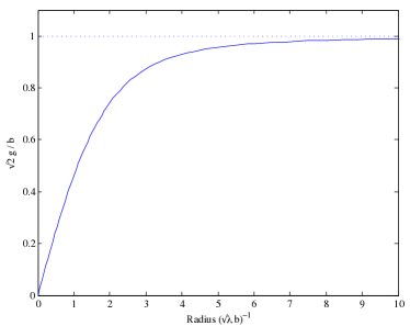
Figure 1: Field configuration for antisymmetric tensor monopole solution. For this solution, $B_{\theta\phi}=-B_{\phi\theta}=g(r)r^{2}\sin\theta$; all other components of $B_{ab}$ vanish.

We can also expand $\tilde{g}$ as a power series in $1/\tilde{r}$ to examine its asymptotic behaviour; the result is

$$\tilde{g}(\tilde{r})=1-\frac{1}{2\tilde{r}^{2}}-\frac{3}{2\tilde{r}^{4}}+\dots.$$ (33)

We also note that the equation (32) is invariant under the transformation $\tilde{g}\to-\tilde{g}$. A solution that asymptotically approaches $g=-b/\sqrt{2}$ rather than $g=b/\sqrt{2}$ can be thought of as an antimonopole rather than a monopole solution.

V Physical properties of Lorentz defect solutions

In the previous section, we found that static, maximally symmetric topological defect solutions exist for two types of tensor fields: vectors and antisymmetric two-tensors. A natural question to ask concerning these solutions regards the form of their stress-energy; the gravitational effects of such solutions would be a natural (and, in the absence of an explicit coupling between these fields and “conventional” matter fields, the only) way to detect them.

V.1 Vector domain walls

In the case of vector fields, we were able to write down an exact solution (28) representing a domain-wall solution of the equations of motion (23). The stress-energy tensor associated with the vector field $A^{a}$ can be found be the usual technique of differentiating the action (14) with respect to the metric:

$$T_{ab}=F_{ac}F_{b}{}^{c}-\frac{1}{2}\eta_{ab}F_{cd}F^{cd}\\ +\lambda\left((A^{c}A_{c}+b^{2})A_{a}A_{b}-\frac{1}{2}\eta_{ab}(A^{c}A_{c}+b^{2})^{2}\right).$$ (34)

Note the presence of the third term here, which arises due to the differentiation of our potential $V(A_{a}A_{b}g^{ab})$ with respect to the metric. Terms such as this do not arise for topological defects constructed out of Lorentz scalars; the fact that our fields are Lorentz tensors requires that our potential depend on the metric as well.

Plugging our solution (28) into (34) yields

$$T_{tt} =\lambda b^{4}\tanh^{2}(\sqrt{-\lambda}bx)\operatorname{sech}^{2}(\sqrt{-\lambda}bx),$$ (35a)

$$T_{xx} =0,$$ (35b)

$$T_{yy}=T_{zz} =\lambda b^{4}\operatorname{sech}^{4}(\sqrt{-\lambda}bx).$$ (35c)

We can take a “thin-wall” limit of this solution by requiring that the wall thickness $(\sqrt{-\lambda}b)^{-1}$ go to zero while the surface energy density and tension of the wall be held constant. These latter two quantities are given by

$$\sigma=\int\mathrm{d}x\,T_{tt}=-\frac{2}{3}\sqrt{-\lambda}b^{3}$$ (36)

and

$$\tau=-\int\mathrm{d}x\,T_{yy}=\frac{4}{3}\sqrt{-\lambda}b^{3}$$ (37)

respectively.

We can now see an important aspect of our domain wall solution: its surface energy density is negative. This stems from the requirement for existence of this solution, noted above, that we take the constant $\lambda$ to be negative rather than positive. The gravitational dynamics of thin domain walls with a general surface density and tension were examined by Ipser and Sikivie Ipser and Sikivie (1984). In particular, it is shown that a domain wall is “attractive” if $\sigma-2\tau>0$, and “repulsive” if $\sigma-2\tau<0$; more precisely, two observers on opposite sides of the wall must accelerate outwards to remain a constant distance apart if $\sigma-2\tau>0$, and must accelerate inwards to remain a constant distance apart if $\sigma-2\tau<0$. Since our vector domain walls have $\sigma-2\tau<0$, they fall into the latter, “repulsive” category.

However, there are some troubling aspects of this solution. Since we were forced to set $\lambda<0$ to allow existence of the solution (28), we can see from (35) that the energy density $\rho=T_{tt}$ and transverse pressure $P_{\perp}=T_{yy}=T_{zz}$ are negative. This implies, in particular, that this solution does not satisfy any of the standard energy conditions (weak, null, strong, or dominant.)

A more serious problem concerns the stability of this theory. Choosing $\lambda<0$ means that the potential $V(A^{a}A_{a})$ is unbounded below rather than unbounded above. In essence, we have inverted the potential; instead of the vacuum manifold lying at the bottom of the brim of a “Mexican hat”, it is instead perched atop a “Bundt cake.” It thus seems likely that a small perturbation will cause our fields to “roll down the hill,” and thus that this domain wall will be unstable.

Further evidence for this can be found by obtaining the Hamiltonian associated with the action (14) for a general potential $V(A^{a}A_{a})$. Taking the field variables to be the components of $A_{a}$, and denoting the spatial components of $A_{a}$ with Roman indices $i,j,k,\dots$, the Hamiltonian can be shown to be

$$H=\int\mathrm{d}^{3}\vec{x}\bigg{[}\frac{1}{2}\Pi^{i}\Pi_{i}+\frac{1}{4}F^{ij}F_{ij}+V(-(A_{0})^{2}+\vec{A}^{2})\\ +2V^{\prime}(-(A_{0})^{2}+\vec{A}^{2})(A_{0})^{2}+\Pi^{0}u\bigg{]},$$ (38)

where the conjugate momenta $\Pi^{i}\equiv F^{i0}$, $u$ is a Lagrange multiplier, and the fields are subject to the constraints

$$\Pi^{0}=0$$ (39)

and

$$\partial_{i}\Pi^{i}+2V^{\prime}(A^{2})A_{0}=0.$$ (40)

If the function $V(x)$ is unbounded below for positive values of its argument $x$, this Hamiltonian can be seen to be unbounded both above and below: it can be made arbitrarily positive by taking $A_{0}\to 0$, $A_{i}\to 0$, and $\Pi^{i}$ to be large but divergence-free, and can be made arbitrarily negative by taking $A_{0}\to 0$, $\Pi^{i}\to 0$, and $A_{i}$ large and slowly varying. This implies that the magnitudes of our fields are not bounded by energy conservation; we must view this as strong evidence that the full field theory (14) with $\lambda<0$ is unstable, and (if so) physically unrealistic.

V.2 AS tensor monopoles

In the case of antisymmetric two-tensor fields, we found a numerical solution (shown in Figure 1) which represents a monopole solution of the theory with the action (15). The physical properties of this solution were briefly discussed in Seifert ; we review and elaborate upon this work here.

The stress-energy tensor associated with the action (15) is

$$T_{ab}=F_{acd}F_{b}{}^{cd}-\frac{1}{6}\eta_{ab}F_{cde}F^{cde}\\ +\lambda\left(4(B_{de}B^{de}-b^{2})B_{ac}B_{b}{}^{c}-\frac{1}{2}\eta_{ab}(B_{cd}B^{cd}-b^{2})^{2}\right).$$ (41)

In terms of the function $g(r)$ defined in (30), the the energy density $\rho=T_{tt}$, the radial pressure $P_{r}=T_{rr}$, and the tangential pressure $P_{\theta}=r^{-2}T_{\theta\theta}$ are

$$\rho =\left(g^{\prime}+\frac{2}{r}g\right)^{2}+\frac{\lambda}{2}(2g^{2}-b^{2})^{2},$$ (42a)

$$P_{r} =\left(g^{\prime}+\frac{2}{r}g\right)^{2}-\frac{\lambda}{2}(2g^{2}-b^{2})^{2},$$ (42b)

$$P_{\theta} =\left(g^{\prime}+\frac{2}{r}g\right)^{2}+\frac{\lambda}{2}\left(8g^{2}(2g^{2}-b^{2})-(2g^{2}-b^{2})^{2}\right).$$ (42c)

It is important to note that while the function $g(r)$ satisfies the same equation of motion as the $O(3)$ scalar monopole described in Barriola and Vilenkin (1989), the form of the stress-energy tensor is rather different. In particular, the $O(3)$ scalar monopole has positive energy density but negative pressures (both radial and tangential), while for our monopole all three quantities ($\rho$, $P_{r}$, and $P_{\theta}$) are everywhere positive (see Figure 2.)

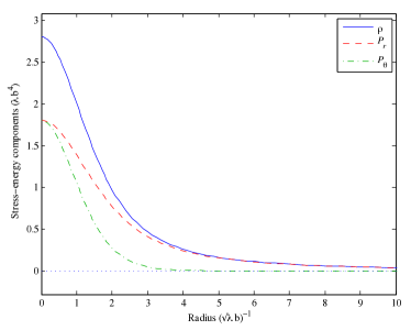
Figure 2: Energy density $\rho$, radial pressure $P_{r}$, and tangential pressure $P_{\theta}$ for the antisymmetric tensor monopole. Note the positivity of all three quantities.

We can use the asymptotic form of $\tilde{g}$ from Equation (33) to see the fall-off properties of the stress-energy components; these work out to be

$$\rho=\lambda b^{4}\left[\frac{4}{\tilde{r}^{2}}+\frac{1}{\tilde{r}^{4}}+\dots\right],$$ (43a)

$$P_{r}=\lambda b^{4}\left[\frac{4}{\tilde{r}^{2}}-\frac{1}{\tilde{r}^{4}}+\dots\right],$$ (43b)

and

$$P_{\theta}=\lambda b^{4}\left[\frac{1}{\tilde{r}^{4}}+\dots\right].$$ (43c)

Note that the fall-off rate of $P_{\theta}$ is significantly faster than that of $\rho$ and $P_{r}$; this is due to an exact cancellation between the $\mathcal{O}(r^{-2})$ dependencies of the kinetic portion and the potential portion of the stress-energy tensor.

This difference in sign between the pressures of the $O(3)$ monopole and our tensor monopole will lead to significant differences when we examine the gravitational effects of this field configuration. In the case of a dynamical metric $g_{ab}$, the tensor equations of motion are

$$(\mathcal{E}_{G})_{ab}\equiv G_{ab}-8\pi G\left[F_{acd}F_{b}{}^{cd}-\frac{1}{6}g_{ab}F_{cde}F^{cde}\right.\\ +\lambda\bigg{(}4(B_{de}B^{de}-b^{2})B_{ac}B_{b}{}^{c}\\ \left.-\frac{1}{2}\eta_{ab}(B_{cd}B^{cd}-b^{2})^{2}\bigg{)}\right]=0$$ (44a)

and

$$(\mathcal{E}_{B})_{ab}\equiv\nabla^{c}F_{cab}-2\lambda(B_{cd}B^{cd}-b^{2})B_{ab}=0.$$ (44b)

Since we are assuming spherical symmetry and staticity, we can use Schwarzschild coordinates to write our line element as

$$ds^{2}=-M^{2}(r)dt^{2}+N^{2}(r)dr^{2}+r^{2}(d\theta^{2}+\sin^{2}\theta d\phi^{2}).$$ (45)

We can use the same ansatz (30) as we did in flat spacetime for the $\theta\phi$-component of $B_{ab}$, and take $B_{tr}$ to vanish. In terms of our ansatz functions $M(r)$, $N(r)$, and $g(r)$, these equations become

$$\frac{2}{\tilde{r}}\frac{N^{\prime}}{N}+\frac{1}{\tilde{r}^{2}}(N^{2}-1)\\ =4\pi Gb^{2}\left(\left(\tilde{g}^{\prime}+\frac{2}{\tilde{r}}\tilde{g}\right)^{2}+\frac{1}{2}N^{2}(\tilde{g}^{2}-1)^{2}\right),$$ (46a)

$$\frac{2}{\tilde{r}}\frac{M^{\prime}}{M}-\frac{1}{\tilde{r}^{2}}(N^{2}-1)\\ =4\pi Gb^{2}\left(\left(\tilde{g}^{\prime}+\frac{2}{\tilde{r}}\tilde{g}\right)^{2}-\frac{1}{2}N^{2}(\tilde{g}^{2}-1)^{2}\right),$$ (46b)

and

$$\frac{\partial}{\partial\tilde{r}}\left(\tilde{g}^{\prime}+\frac{2}{\tilde{r}}\tilde{g}\right)+\left(\frac{M^{\prime}}{M}-\frac{N^{\prime}}{N}\right)\left(\tilde{g}^{\prime}+\frac{2}{\tilde{r}}\tilde{g}\right)\\ -N^{2}(\tilde{g}^{2}-1)\tilde{g}=0,$$ (46c)

where we have rescaled our coordinates and fields as in the flat spacetime case; primes denote differentiation with respect to $\tilde{r}$.

These equations do not have an obvious closed-form solution. However, we can obtain some interesting information concerning the asymptotic properties of these solutions by taking the BPS limit Bogomol’nyi (1976); Prasad and Sommerfield (1975), in which we set $\tilde{g}\to 1$ exactly; this corresponds to taking $\lambda\to 0$ while still looking for solutions with the asymptotic behaviour of a topological defect. In this limit, the components of the Einstein equation (46a) and (46b) become

$$\frac{2}{\tilde{r}}\frac{N^{\prime}}{N}+\frac{1}{\tilde{r}^{2}}(N^{2}-1) \approx\frac{\epsilon}{\tilde{r}^{2}},$$ (47)

$$\frac{2}{\tilde{r}}\frac{M^{\prime}}{M}-\frac{1}{\tilde{r}^{2}}(N^{2}-1) \approx\frac{\epsilon}{\tilde{r}^{2}},$$ (48)

where we have defined $\epsilon\equiv 16\pi Gb^{2}$. These equations have the exact solution

$$M^{2}(r) =C_{2}\frac{\tilde{r}^{1+\epsilon}+C_{1}}{\tilde{r}^{1-\epsilon}},$$ (49)

$$N^{2}(r) =(1+\epsilon)\frac{\tilde{r}^{1+\epsilon}}{\tilde{r}^{1+\epsilon}+C_{1}},$$ (50)

where $C_{1}$ and $C_{2}$ are constants of integration. (Note that $C_{2}$ can be set to an arbitrary positive value via a rescaling of $t$; we will henceforth set $C_{2}=1$.)

It is important to note that the stress-energy fall-off properties of this solution are not quite the same as those in flat spacetime. Asymptotically, the energy density $\rho$ and radial pressure $P_{r}$ are given by

$$\rho\approx P_{r}\approx N^{-2}\frac{4g^{2}}{r^{2}}\approx\frac{4\lambda b^{4}}{\tilde{r}^{2}},$$ (51)

which are the same as in the flat spacetime case. However, the fall-off rate of the tangential pressure $P_{\theta}$ must change; in spherical coordinates, the Bianchi identity implies that

$$\nabla^{\mu}T_{\mu r}=\frac{\partial P_{r}}{\partial r}+\frac{M^{\prime}}{M}(\rho+P_{r})+\frac{2}{r}(P_{r}-P_{\theta})=0$$ (52)

Plugging in our asymptotic expressions for $\rho$, $P_{r}$, and $M$, we see that in curved spacetime $P_{\theta}$ must have the asymptotic form

$$P_{\theta}\approx\frac{\epsilon}{2}(\rho+P_{r})\approx\frac{4\epsilon\lambda b^{4}}{\tilde{r}^{2}}.$$ (53)

If our mass scale $b$ is significantly smaller than the Planck mass, we will still have $P_{\theta}\ll\rho$ and $P_{\theta}\ll P_{r}$ asymptotically, as we did in flat spacetime. However, the introduction of a curved metric requires that the fall-off rate of $P_{\theta}$ change from $r^{-4}$ to $r^{-2}$.

Returning to the case of non-zero $\lambda$, we expect that our solution will still have the same asymptotic behaviour, with $M(r)\propto\tilde{r}^{\epsilon}$ and $N(r)\to\sqrt{1+\epsilon}$. The fact that $N$ does not go to unity as $r\to\infty$ implies that the constant-time slices of this spacetime have a spherical deficit angle; specifically, the equatorial plane (i.e., $\theta=\pi/2$) has the asymptotic geometry of a cone with a deficit angle $\pi\epsilon$. The divergence of the $g_{tt}$ component of the metric might seem to be a cause for concern; it does not appear that, for example, such a metric could be asymptotically flat. For a monopole in isolation, this could imply that the full solution is inherently non-static; an analogous situation would be that of anti-de Sitter space in Schwarzschild coordinates, in which the $tt$-component of the metric diverges proportionally to $r^{2}$. It can also be shown that various curvature invariants of our metric go to zero as $r\to\infty$; the Ricci scalar is proportional to $r^{-2}$ (as might be expected from the stress-energy tensor), and the squares of the Ricci tensor and the Riemann tensor both fall off as $r^{-4}$.

Moreover, in a realistic physical situation, we only expect this solution to be valid out to some finite radius where the effects of larger structure (on galactic or cosmic scales) take over. Unless the mass scale $b$ of the tensor field is close to the Planck scale, we will have $\epsilon\ll 1$, and the growth of $g_{tt}$ should be sufficiently slow that we can “patch” our solution into one describing the appropriate larger-scale structure. Thus, although this solution behaves oddly in the asymptotic region, its behaviour does not seem bad enough to reject it as unphysical.

With this asymptotic geometry found, we can now ask what its effects on the propagation of test particles (particularly light rays) might be. Assuming that our tensor field $B_{ab}$ does not couple directly to the Maxwell field, a light ray propagating in this background will follow a null geodesic. Without loss of generality, we can assume that this geodesic lies in the equatorial plane (i.e., $\theta=\pi/2$.) Since our spacetime is static and spherically symmetric, it has two Killing vector fields $t^{a}$ and $\phi^{a}$ (the generators of timelike translations and rotations in the equatorial plane, respectively) giving rise to two constants of the motion:

$$E =-u^{a}t_{a}, L =u^{a}\phi_{a},$$ (54)

where $u^{a}$ is the four-velocity of the particle.

Two possible physical effects spring to mind that might arise in a geometry such as this one: gravitational redshift and deflection of light rays. Using standard techniques Wald (1984), it can be shown that a light ray emitted with frequency $\omega_{e}$ at some distance $r_{e}$ from the monopole will be observed to have a frequency $\omega_{o}$ by an observer at a distance $r_{o}$ from the monopole, where

$$\frac{\omega_{o}}{\omega_{e}}=\frac{M(r_{e})}{M(r_{o})}=\left(\frac{r_{e}}{r_{o}}\right)^{\epsilon}.$$ (55)

If $\epsilon\ll 1$, the first-order fractional redshift $\Delta\omega/\omega_{e}$ will then be

$$\frac{\Delta\omega}{\omega_{e}}\approx\epsilon\ln\left(\frac{r_{e}}{r_{o}}\right).$$ (56)

We can see that any gravitational redshift due to the presence of the monopole will be quite small, especially if $r_{e}$ and $r_{o}$ are close to the same order of magnitude. Even if $r_{e}$ and $r_{o}$ are unrealistically disparate in size—say, the Planck distance and the Hubble distance, respectively—we would still have $\ln(r_{e}/r_{o})\approx 140$, and a mass scale $b$ that was more than a few orders of magnitude less than the Planck scale would still make this redshift extremely difficult to detect.

The situation for the deflection of light by the spacetime curvature is somewhat more interesting. We again use the standard techniques Wald (1984) to derive the motion of massless particles. A null geodesic in the equatorial plane will satisfy

$$-M^{2}(r)\dot{t}^{2}+N^{2}(r)\dot{r}^{2}+r^{2}\dot{\phi}^{2}=0,$$ (57)

where a dot over a symbol denotes the derivative of the particle’s coordinate position $(t(s),r(s),\pi/2,\phi(s))$ with respect to some affine parameter $s$ on the worldline. The constants of the motion (54) are given by $E=M^{2}\dot{t}$ and $L=r^{2}\dot{\phi}$; we can thus write

$$\dot{r}^{2}+\left[\frac{L^{2}}{N^{2}r^{2}}-\frac{E^{2}}{M^{2}N^{2}}\right]=0.$$ (58)

Using the asymptotic forms of $M$ and $N$ found above (with $C_{1}\to 0$), we see that the path of the null geodesic satisfies

$$\frac{d\phi}{dr}=\frac{\dot{\phi}}{\dot{r}}=\pm\frac{\sqrt{1+\epsilon}}{r^{2}\sqrt{\beta^{-2}(\sqrt{2\lambda}b)^{-2\epsilon}r^{-2\epsilon}-r^{-2}}}.$$ (59)

where $\beta\equiv L/E$. We can then find the total angular deflection of this geodesic by integrating this quantity over $r$ from $\infty$ to $r_{m}$ (the value of $r$ for which the denominator of (59) vanishes) and doubling it (to account for both the deflection incurred travelling from $r=\infty$ to $r=r_{m}$ and the deflection incurred in travelling back to $r=\infty$.) The result is

$$\Delta\phi=\pi\frac{\sqrt{1+\epsilon}}{1-\epsilon},$$ (60)

or, defining $\delta\phi\equiv\Delta\phi-\pi$ to be the angle between the “unperturbed” and “perturbed” directions of propagation,

$$\delta\phi\approx\frac{3\pi}{2}\epsilon.$$ (61)

We see that to leading order in $\epsilon$, the deflection angle $\delta\phi$ does not depend on $\beta$, and thus is independent of the properties of the geodesic. In other words, with respect to the propagation of light, at lowest order this spacetime behaves as though it has a solid deficit angle but is otherwise flat. This “apparent deficit angle” is not the same as the deficit angle of the constant-time slices mentioned above; it arises from both the deficit angle in the spatial geometry and from the behaviour of the $tt$-component of the metric (roughly analogous to the gravitational potential.) From an observational point of view, however, the light-bending signature of one of our antisymmetric tensor monopoles would be exactly the same as that of the previously examined $O(3)$ scalar monopoles Barriola and Vilenkin (1989); only the dependence of the deflection angle on the respective mass scales of the two models differs.

VI Discussion

We have examined the existence and properties of topological defect solutions arising from a spacetime tensor which spontaneously breaks Lorentz symmetry by acquiring a fixed norm $\mathcal{T}_{(a)}\mathcal{T}^{(a)}=C$ in vacuum. For topological defect solutions to exist, the set of such tensor fields (the vacuum manifold) must contain a non-contractible $S^{0}$, $S^{1}$, or $S^{2}$; we found that the only tensors with rank not greater than five and of definite symmetry type with this topology are vectors, antisymmetric two-tensors, and symmetric two-tensors. From these, we obtained domain wall solutions in which a vector takes on a negative (timelike) norm asymptotically, and monopole solutions in which an antisymmetric two-tensor takes on a positive norm asymptotically. These vector domain wall solutions appear to be unstable; however, the antisymmetric two-tensor monopole solutions are well-behaved in flat spacetime, and can give rise to observable light-bending effects.

It is notable that we have not found any cosmic string solutions in our work. Such solutions would require the signature of our tensor space to have either $n_{+}=2$ or $n_{-}=2$; consulting Table 1, we see that no such tensor with $r\leq 5$ exists. It is unclear whether a deep mathematical reason exists for this lacuna; such a tensor space might exist at higher rank, but this seems unlikely.

If cosmic string solutions are desired, two approaches are still open. The first is simply to combine multiple fields. Rather than having a single tensor field $\mathcal{T}^{(a)}$ with a potential minimized at $\mathcal{T}_{(a)}\mathcal{T}^{(a)}=C$, we can envision two tensor fields $(\mathcal{T}_{1})^{(a)}$ and $(\mathcal{T}_{2})^{(a)}$ with a combined potential that is minimized when

$$(\mathcal{T}_{1})^{(a)}(\mathcal{T}_{1})_{(a)}\pm(\mathcal{T}_{2})^{(a)}(\mathcal{T}_{2})_{(a)}=C.$$ (62)

If the respective signatures of the tensor spaces in which $(\mathcal{T}_{1})^{(a)}$ and $(\mathcal{T}_{2})^{(a)}$ lie are $(n_{1+},n_{1-})$ and $(n_{2+},n_{2-})$, respectively, then it is not hard to see that the “effective” signature of the combined tensor space is $(n_{1+}+n_{2\pm},n_{1-}+n_{1\mp})$. Thus, by combining two or more fields such that some linear combination of their norms is minimized, we could in principle obtain a vacuum manifold with an “effective” $n_{+}$ or $n_{-}$ equal to two.

Unfortunately, an examination of Table 1 shows that the only two types of tensor fields with $n_{+}\leq 2$ or $n_{-}\leq 2$ are scalar and vector fields (or fields equivalent to these.) The case of two scalar fields (or a single complex scalar field) is already well-known, and does not violate Lorentz symmetry in the sense we are interested in. A theory containing a scalar field and a vector field, in a potential that is minimized when $A^{a}A_{a}-\phi^{2}=-b^{2}$, would have a non-contractible $S^{1}$ in its vacuum manifold; so would a theory of a complex vector field (effectively, two independent vector fields) with $A^{a}A^{*}_{a}=-b^{2}$. However, since we would still be using the timelike components of the vector fields to construct our topological defect, we would again need to “invert” the potential (as in the case of a single vector field) to obtain a global solution. Such theories would likely then share the same instability that our original vector domain-wall model had.

The other option to obtain cosmic string solutions would be to generalize our vacuum manifolds. Throughout this work, we have been examining only those sets of tensors for which the “square” of the tensor is some constant value. It is plausible that some other invariant (of higher order than quadratic in the tensor field) could give a vacuum manifold of the correct topology to support cosmic string defects. Additionally, more complicated potentials could give rise to defect types that would be impossible via a simple “sum of norms” vacuum manifold of the form (62); an example of this, in which two spacelike vector fields form a domain wall solution, was described in Chkareuli et al. (2009). Such manifolds could be expressed as the set of zeroes of one or more polynomials in $\mathbb{R}^{n}$ for some $n$, also known as a real algebraic variety. Unfortunately, it does not appear that any known characterization of the topology of such spaces is as complete as that for the quadratic case; see Bochnak et al. (1998) for more details.

Both of the solutions we have found were obtained under the assumption of the maximal symmetry compatible with the type of defect solution we sought: planar symmetry in the domain wall case, spherical symmetry in the monopole case, and staticity in both cases. It is likely that that interesting solutions with a lesser degree of symmetry might also exist in these theories, especially if one relaxes the staticity requirement; one could look at linearized solutions about these backgrounds and investigate their evolution. (As noted above, the evolution of perturbations of a domain wall is likely to be unbounded.) It is also conceivable that solutions with reduced spatial symmetry but which are still static might also exist, both for these theories and for theories containing symmetric tensors and spacelike vector fields. (We previously rejected these latter two types of fields as uninteresting due to their lack of symmetric solutions.) Intuitively, such solutions would seem less likely to exist, and would most likely be of higher energy than the symmetric solutions of the theory; certainly, such solutions would not be “close” in any real sense to the symmetric solutions we have found.

In previous work on topological defects, it has been useful to draw a distinction between “global” monopoles, in which a global symmetry is broken, and “gauge” monopoles, in which a local symmetry is broken. In the present case, it is unclear how useful this distinction is. In the case of a fixed flat background, the Lorentz and Poincaré symmetries of the Lagrangian are global ones, so in this case we can classify our solutions as global monopoles. Since diffeomorphism symmetry can be thought of as “gauged Poincaré symmetry” Kibble (1961), one could then say that a gauged solution is one where the Levi-Citiva connection and (by extension) the metric are dynamical fields; from this perspective, a gravitating monopole is a gauge monopole. However, unlike in the case of scalar monopoles, the passage from global symmetry to gauge symmetry does not greatly change the behaviour of the original global monopole solutions. In particular, the $O(3)$ scalar monopoles have an energy (i.e., the integral of the energy density over all of space) that is formally infinite, due to the $r^{-2}$ fall-off rate of the energy density $\rho$. This infinity is eliminated when this $O(3)$ symmetry is promoted to a gauge symmetry, as the parts of the fields that cause the divergence can in effect be “gauged away”. In contrast, our antisymmetric tensor monopoles retain the same energy density fall-off properties when we promote the metric to a dynamical field, and so are not cured of their formally divergent energies. It therefore seems that the distinction between global and gauge monopoles is not as physically relevant in the present case as it is in the case of internal symmetries.

The experimental prospects for the observation of these antisymmetric tensor monopoles will, of course, depend critically on their current abundance in the Universe. We would expect that such topological defects would have formed in a phase transition as the Universe cooled after the Big Bang, via the Kibble mechanism Kibble (1976). To within an order of magnitude, one such structure should form in each Hubble volume at the time of this phase transition. However, it is not clear how efficiently these structures might recombine in the subsequent evolution of the Universe. Much of Barriola & Vilenkin’s discussion Barriola and Vilenkin (1989) concerning the recombination of global $O(3)$ monopoles applies here. Since these are global monopoles, the characteristic energy scale of a monopole-antimonopole pair will be directly proportional to the distance separating them; the effective force between them will then be independent of distance. This would seem to imply that pair-annihilation of such structures would be quite efficient. It is unclear, however, how easily these monopoles can “find each other” in an expanding Universe. As in the $O(3)$ case, a numerical simulation will probably be required to answer the question of current abundance of AS tensor monopoles. Simulations in the $O(3)$ case Bennett and Rhie (1990) have shown that the density of such monopoles remains roughly constant at approximately $(4.0\pm 1.5)d_{H}^{-3}$, where $d_{H}$ is the horizon distance, as the Universe evolves; it seems plausible that similar results (up to an order of magnitude) will obtain in our case.

Appendix A Derivation of tensor space signatures

In Table 1, we gave a list of the signatures $(n_{+},n_{-})$ of tensor spaces with rank $r\leq 5$ and definite symmetry pattern. We now present the method by which these signatures were found. Much of what follows, particularly in the first subsection, is based on the classic texts by Hamermesh Hamermesh (1962) and by Weyl Weyl (1939).

A.1 Preliminaries

A.1.1 Representations of $GL(d)$

Let $V$ denote a $d$-dimensional real vector space, and let $\mathbb{U}_{r}$ denote the tensor product of $V$ with itself $r$ times; in other words, the elements of $\mathbb{U}_{r}$ are the rank-$r$ contravariant tensors on $V$. This space is itself a $d^{r}$-dimensional vector space: it is closed under addition and multiplication by real numbers.

Consider now the group of all non-singular linear transformations on $V$, denoted by $GL(d)$. The action of this group on $V$ extends in a natural way to the tensor space $\mathbb{U}_{r}$. (Roughly speaking, given an element $g\in GL(d)$, we can act on each “copy” of $V$ in $\mathbb{U}_{r}$ with $g$.) This group action can be seen to be a faithful representation of $GL(d)$ with $\mathbb{U}_{r}$ as its representation space. It is further known that this representation is reducible, i.e., the space $\mathbb{U}_{r}$ can be written as

$$\mathbb{U}_{r}=\bigoplus_{i}\mathbb{V}_{i},$$ (63)

such that each subspace $\mathbb{V}_{i}$ is closed under the above described action of $GL(d)$.

These subspaces $\mathbb{V}_{i}$ are essentially obtained by resolving an arbitrary tensor into tensors with some symmetry among their indices. A familiar example of this is the case $r=2$: an arbitrary tensor $t^{ab}$ can be resolved into two parts, one symmetric and one antisymmetric, i.e.,

$$t^{ab}=t^{(ab)}+t^{[ab]}.$$ (64)

We can write this in terms of projectors on the space of tensors; defining

$$(P_{S})^{a_{1}a_{2}}{}_{b_{1}b_{2}}=\frac{1}{2}(\eta^{a_{1}}{}_{b_{1}}\eta^{a_{2}}{}_{b_{2}}+\eta^{a_{1}}{}_{b_{2}}\eta^{a_{2}}{}_{b_{1}})$$ (65)

and

$$(P_{A})^{a_{1}a_{2}}{}_{b_{1}b_{2}}=\frac{1}{2}(\eta^{a_{1}}{}_{b_{1}}\eta^{a_{2}}{}_{b_{2}}-\eta^{a_{1}}{}_{b_{2}}\eta^{a_{2}}{}_{b_{1}}),$$ (66)

it is not hard to show that

$$(P_{S})^{a_{1}a_{2}}{}_{b_{1}b_{2}}(P_{S})^{b_{1}b_{2}}{}_{c_{1}c_{2}}=(P_{S})^{a_{1}a_{2}}{}_{c_{1}c_{2}},$$ (67a)

$$(P_{A})^{a_{1}a_{2}}{}_{b_{1}b_{2}}(P_{A})^{b_{1}b_{2}}{}_{c_{1}c_{2}}=(P_{A})^{a_{1}a_{2}}{}_{c_{1}c_{2}},$$ (67b)

$$(P_{S})^{a_{1}a_{2}}{}_{b_{1}b_{2}}(P_{A})^{b_{1}b_{2}}{}_{c_{1}c_{2}}=(P_{A})^{a_{1}a_{2}}{}_{b_{1}b_{2}}(P_{S})^{b_{1}b_{2}}{}_{c_{1}c_{2}}=0,$$ (67c)

and

$$(P_{S})^{a_{1}a_{2}}{}_{b_{1}b_{2}}+(P_{A})^{a_{1}a_{2}}{}_{b_{1}b_{2}}=\eta^{a_{1}}{}_{b_{1}}\eta^{a_{2}}{}_{b_{2}}.$$ (68)

Thus, $(P_{S})^{a_{1}a_{2}}{}_{b_{1}b_{2}}$ and $(P_{A})^{a_{1}a_{2}}{}_{b_{1}b_{2}}$ are projectors in the $d^{2}$-dimensional space of two-tensors on $V$. $(P_{S})^{(a)}{}_{(b)}$ projects an arbitrary tensor $t^{ab}$ to its symmetric part, while $(P_{A})^{(a)}{}_{(b)}$ projects $t^{ab}$ onto its antisymmetric part. We can denote the subspaces projected onto by $(P_{S})^{(a)}{}_{(b)}$ and $(P_{A})^{(a)}{}_{(b)}$ as $\mathbb{V}_{S}$ and $\mathbb{V}_{A}$, respectively. Moreover, the action of $GL(d)$ will map symmetric tensors to symmetric tensors and antisymmetric tensors to antisymmetric tensors; thus, $\mathbb{V}_{S}$ and $\mathbb{V}_{A}$ are closed under the action of $GL(d)$.

To generalize this to higher-rank tensors, we must first introduce an algebra acting on $\mathbb{U}_{r}$. Let $S_{r}$ be the group of permutations on $r$ objects, and let $\mathfrak{s}_{r}$ be the $r!$-dimensional vector space spanned by tensors of the form

$$\eta^{a_{\sigma(1)}}{}_{b_{1}}\eta^{a_{\sigma(2)}}{}_{b_{2}}\cdots\eta^{a_{\sigma(r)}}{}_{b_{r}}\equiv\eta^{(a_{\sigma(i)})}{}_{(b_{i})}$$ (69)

for some permutation $\sigma\in S_{r}$. The action of $\eta^{(a_{\sigma(i)})}{}_{(b_{i})}$, when contracted with a tensor $F^{(b_{i})}$, is simply to return that tensor with its indices rearranged by the permutation $\sigma$. By definition, we can add two elements of $\mathfrak{s}_{r}$ together to form another element of $\mathfrak{s}_{r}$, or multiply any element by a real number. However, we can also multiply elements of $\mathfrak{s}_{r}$ together in a natural way: if $a=\eta^{(a_{\sigma(i)})}{}_{(b_{i})}$ is a basis element corresponding to a permutation $\sigma\in S_{r}$ and $b=\eta^{(a_{\tau(i)})}{}_{(b_{i})}$ corresponds to $\tau\in S_{r}$, then we can define the product of $a$ and $b$ as

$$ab=\eta^{(a_{\sigma(i)})}{}_{(b_{i})}\eta^{(b_{\tau(i)})}{}_{(c_{i})}=\eta^{(a_{\sigma(\tau(i))})}{}_{(c_{i})},$$ (70)

since $\eta^{(a_{\sigma(i)})}{}_{(b_{i})}=\eta^{(a_{\sigma(\tau(i))})}{}_{(b_{\tau(i)})}$. (This can be seen by an appropriate rearrangement of the $\eta$’s in the definition (69) above.) When viewed in terms of its action of $\mathbb{U}_{r}$, this implies that acting on $F^{(a)}$ by the element of $\mathfrak{s}$ associated with $\tau$, followed by that element associated with $\sigma$, yields $F^{(a)}$ with its indices permuted by $\sigma\tau$, exactly as one would expect. The multiplication of two arbitrary vectors in $\mathfrak{s}_{r}$ is then given by requiring distributivity to hold for our multiplication operator, i.e., $(a+b)c=ac+bc$ and $c(a+b)=ca+cb$ for all $a$, $b$, and $c$ in $\mathfrak{s}_{r}$.

Not all elements in $\mathfrak{s}_{r}$ are associated with strict permutations; a general element of $\mathfrak{s}_{r}$, when contracted with a tensor $F^{(a)}$, will return some linear combination of the various index permutations of $F^{(a)}$. Such linear combinations are what are required to describe the decomposition of $\mathbb{U}_{r}$ into irreducible subspaces under $GL(d)$. In the $r=2$ example above, we found two elements of $\mathfrak{s}_{2}$, $(P_{S})^{(a)}{}_{(b)}$ and $(P_{A})^{(a)}{}_{(b)}$, which acted as projectors on the space $\mathbb{U}_{2}$ (67); moreover, these projectors resolved the identity (68). In general, it can be shown that such a set of projectors $Y_{i}\in\mathfrak{s}_{r}$, called Young symmetrizers, exists for arbitrary $r$; these symmetrizers can be constructed by means of Young tableaux, and each symmetrizer has associated with it a particular Young tableau. For further details, the interested reader is referred to Hamermesh Hamermesh (1962).

A.1.2 $GL(d)\to GL(d-1)$ decomposition

The signature of the metric $\eta_{(a)(b)}$ on an irreducible $GL(d)$ subspace $\mathbb{V}$ is, of course, an indefinite metric; roughly speaking, every “time” component of a tensor gives a negative sign, while the “space” components give positive signs. It will therefore be advantageous to look at how a given tensor representation behaves under purely “spatial” transformations, i.e., those which act on the some set of positive-norm coordinates $\{x^{1},x^{2},\dots,x^{d-1}\}$ while leaving the negative-norm “time” coordinate $x^{d}$ invariant.

Under this subgroup $GL(d-1)\subset GL(d)$, each irreducible subspace $\mathbb{V}$ will split into the direct sum of several subspaces $\mathbb{W}_{i}$, each of which is invariant under $GL(d-1)$:

$$\mathbb{V}=\bigoplus_{i}\mathbb{W}_{i}.$$ (71)

These subspaces are themselves equivalent (in terms of their behaviour under $GL(d-1)$) to tensor spaces of definite symmetry type; specifically, the Young tableaux of the subspaces can be obtained by removing one box from the bottom of some or all of the columns of the Young tableau corresponding to $\mathbb{V}$, making sure that the resultant pattern is in fact a valid tableau. For example, we have

$$\yng(2,2)\to\yng(2,2)\oplus\yng(2,1)\oplus\yng(2).$$ (72)

To see this, consider the “standard components” of a tensor in $\mathbb{V}$, i.e., a complete set of components which determine all the others via the symmetry relations on $\mathbb{V}$. If $\mathbb{V}$ is the image of some Young symmetrizer $Y$, the standard components of a tensor in $\mathbb{V}$ are found by taking the standard tableau corresponding to $Y$ and filling with the symbols $\{1,\dots,d\}$ such that the symbols are non-decreasing along the rows and strictly increasing down the columns. Importantly, this means that the symbol $d$ will only appear at the bottom of a column in such a filling. We can then consider the subspace of $\mathbb{V}$ spanned by the set of tensors $\{(e_{i})^{(a)}\}_{\mathbb{V}}$, where the non-vanishing standard components of each tensor $(e_{i})^{(a)}$ are those with $d$’s at the bottom of a certain subset of the columns in the Young tableau for $\mathbb{V}$. Since the action of $GL(d-1)$ effectively “leaves $d$’s alone”, such a subspace will be invariant under the action of $GL(d-1)$.

A.1.3 $GL(d)\to O(d-1,1)$ decomposition

We have thus far been examining the properties of tensors in $\mathbb{U}_{r}$ under arbitrary invertible transformations on the underlying vector space $V$. However, this symmetry group is not the physically relevant one. Rather, we expect our physical laws to be invariant under the actions of the Lorentz subgroup $O(d-1,1)\subset GL(d)$, defined as that subgroup of $GL(d)$ which leaves the spacetime metric $\eta_{ab}$ (and, by extension, the tensor metric $\eta_{(a)(b)}$) invariant. As in the $GL(d-1)\subset GL(d)$ case, an irreducible space $\mathbb{V}$ will decompose into another set of invariant subspaces $\bar{\mathbb{W}}_{i}$:

$$\mathbb{V}=\bigoplus_{i}\bar{\mathbb{W}}_{i}.$$ (73)

(These spaces $\bar{\mathbb{W}}_{i}$ will not generically be the same as the $GL(d-1)$ irreducible spaces $\mathbb{W}_{i}$.) Without loss of generality, let the Young symmetrizer $Y$ for $\mathbb{V}$ be obtained from a standard filling of a Young tableau in which as many of the pairs $\{\{a_{1},a_{2}\}$, $\{a_{3},a_{4}\}$, $\{a_{5},a_{6}\}\dots\}$ as possible are in the same row; in other words, the resultant tensors will be symmetric under the exchange of $a_{1}$ and $a_{2}$, of $a_{3}$ and $a_{4}$, and so forth. In general, we can then decompose an arbitrary tensor $F^{(a)}\in\mathbb{V}$ into its components in invariant subspaces under $\bar{\mathbb{W}}_{i}$ by applying the Young symmetrizer to products of the inverse metric $\eta^{ab}$ and trace-free tensors $(f_{i})$ of rank $r,r-2,r-4,\dots$:

$$F^{(a)}=f_{1}^{(a)}+Y^{(a)}{}_{(b)}\left[\sum_{i}\eta^{b_{1}b_{2}}(f_{i})^{b_{3}\dots b_{r}}\right]\\ +Y^{(a)}{}_{(b)}\left[\sum_{i}\eta^{b_{1}b_{2}}\eta^{b_{3}b_{4}}(f_{i})^{b_{5}\dots b_{r}}\right]+\dots.$$ (74)

Moreover, these tensors $(f_{i})$ can each be taken be of definite symmetry type, with a Young pattern of their own; in other words, they lie within some irreducible $GL(d)$ component of $\mathbb{U}_{r-2t}$ for some $t$.

In general, a Ferrers diagram $\{\lambda^{\prime}_{1},\dots,\lambda^{\prime}_{m^{\prime}}\}$ will appear on the right-hand side of the $GL(d)\to O(d-1,1)$ decomposition of an arbitrary Ferrers diagram $\{\lambda_{1},\dots,\lambda_{m}\}$ if $\{\lambda_{1},\dots,\lambda_{m}\}$ is contained in the tensor product of $\{\lambda^{\prime}_{1},\dots,\lambda^{\prime}_{m^{\prime}}\}$ and $\{\delta_{1},\dots,\delta_{m^{\prime\prime}}\}$, where all the integers $\delta_{i}$ are even. If it is possible to multiply $N>1$ such diagrams $\{\delta_{1},\dots,\delta_{m^{\prime\prime}}\}$ with $\{\lambda^{\prime}_{1},\dots,\lambda^{\prime}_{m^{\prime}}\}$ to obtain $\{\lambda_{1},\dots,\lambda_{m}\}$, then there will be $N$ distinct subspaces with the Ferrers diagram $\{\lambda^{\prime}_{1},\dots,\lambda^{\prime}_{m^{\prime}}\}$ in the decomposition. However, this only occurs for $r\geq 6$; for $r\leq 5$, the invariant subspaces are uniquely labelled by their symmetry types. See Littlewood (1950); Jahn (1950) for further details.

As an example, if $\mathbb{V}$ is the space of all tensors with symmetry type given by the Ferrers diagram $\{3,1\}$, it can be shown that

$$\yng(3,1)\to\yng(3,1)\oplus\yng(2)\oplus\yng(1,1).$$ (75)

In other words, $\mathbb{V}$ decomposes into three invariant subspaces under $O(d-1,1)$: the space of all trace-free tensors in $\mathbb{V}$, a space equivalent under $O(d-1,1)$ to the space of all trace-free symmetric two-tensors, and a space equivalent to the space of all antisymmetric two-tensors. The decomposition (74) of an arbitrary tensor in $F^{(a)}\in\mathbb{V}$ would then have three terms on the right-hand side, one corresponding to each of its components in each subspace $\bar{\mathbb{W}}_{i}$. One of these terms would be the trace-free rank-4 tensor $f_{1}^{a_{1}a_{2}a_{3}a_{4}}$. The other two would come from the first sum in (74); they would each be expressible as the product of $\eta^{a_{1}a_{2}}$ with a rank-two tensor ($f_{2}^{a_{3}a_{4}}$, a symmetric trace-free tensor, and $f_{3}^{a_{3}a_{4}}$, an antisymmetric tensor, respectively) and appropriately symmetrized by $Y^{(a)}{}_{(b)}$.

A.2 Signatures of tensor spaces

A.2.1 General tensor spaces

As noted in Section III above, the “tensor norm” given in (6) can be thought of as a quadratic form on $\mathbb{U}_{r}$ or any subspace thereof. If we are dealing with the entire space $\mathbb{U}_{r}$ of rank-$r$ tensors, we can easily construct a basis for this space; simply pick orthonormal coordinates $\{x^{1},x^{2},\dots x^{d}\}$ on our space $V$. We can then construct a set of $d^{r}$ tensors $\{(e_{i})^{(a)}\}\subset\mathbb{U}_{r}$ for each one of which a single coordinate component $F^{\mu_{1}\mu_{2}\cdots\mu_{r}}$ is set to unity and the rest vanish. These tensors can be seen to be an orthonormal basis for $\mathbb{U}_{r}$ under the quadratic form induced by $\eta_{(a)(b)}$. Moreover, since the signature of our spacetime $(n_{+},n_{-})$ is $(d-1,1)$, it is not hard to describe which basis elements have positive norm and which have negative norm. If the non-vanishing component $F^{(\mu)}$ of one of our basis tensors has an even number of “time indices” (i.e., if an even number of the $\mu_{i}$ equal $d$), then the norm of this tensor will contain an even number of factors of $\eta_{dd}$ and will be positive. Similarly, if the non-vanishing component has an odd number of time indices, the norm of this tensor will be negative. Some combinatorics then shows that the number of basis tensors with positive norm is

$$n_{+}=\frac{1}{2}(d^{r}+(d-2)^{r}),$$ (76)

while the number of basis tensors with negative norm is

$$n_{-}=\frac{1}{2}(d^{r}-(d-2)^{r}).$$ (77)

For $d=4$, the signatures $(n_{+},n_{-})$ for $r=\{0,1,2,3,\dots\}$ will be $\{(1,0),(3,1),(10,6),(36,28),\dots\}$.

We have thus found the signature $(n_{+},n_{-})$ of the space $\mathbb{U}_{r}$ of all tensors of rank $r$. However, we noted in the previous subsection that the space $\mathbb{U}_{r}$ decomposes into the direct sum of several spaces $\mathbb{V}_{i}$ of fixed symmetry type. It is natural then to ask what the signature of the metric $\eta_{(a)(b)}$, confined to one of these subspaces (call it $\mathbb{V}$), is. However, it is not immediately obvious how to construct a basis for $\mathbb{V}$ that is orthonormal under $\eta_{(a)(b)}$, or even that such a basis exists (for all we know, $\eta_{(a)(b)}$ might be degenerate on $\mathbb{V}$.)

A clue as to how to proceed can be gleaned from our treatment of the signature of $\mathbb{U}_{r}$ above. Consider subspace of $\mathbb{U}_{r}$ spanned by the subset of all of the basis tensors $\{(e_{i})^{(a)}\}$ whose non-vanishing component has a certain subset of the indices $\mu_{i}$ equal to $d$ and the rest differing from $d$. (For example, for an arbitrary two-tensor $t^{ab}$, we might consider those basis elements for which $t^{1d},t^{2d},\dots t^{(d-1)d}$ are non-vanishing; $t^{dd}$ and $t^{d1}$ would be in the spanning set of different such subspaces.) While these subspaces (call them $\bar{\mathbb{U}}_{i}$) are not invariant under an arbitrary linear transformation in $GL(d)$, the subgroup $GL(d-1)$ which leaves the timelike vector $(0,0,\dots,0,1)$ invariant will also leave each $\bar{\mathbb{U}}_{i}$ invariant. Moreover, we can see that the quadratic form induced by $\eta_{(a)(b)}$ is either positive or negative definite on each such subspace, and that the sign of $\eta_{(a)(b)}$ on each subspace is determined by the number of “time components” corresponding to each subspace.

We wish to find a similar procedure for an invariant $GL(d)$ subspace $\mathbb{V}$, by using the $GL(d)\to GL(d-1)$ decomposition described in Section A.1.2. The first complication arises when we try to determine the orthogonality of the irreducible subspaces $\mathbb{W}_{i}$. In the case of the above decomposition of $\mathbb{U}_{r}$, it was fairly evident that the irreducible $GL(d-1)$ subspaces $\bar{\mathbb{U}}_{i}$ were orthogonal; thus, the union of the orthonormal bases for these subspaces formed an orthonormal basis for $\mathbb{U}_{r}$, and we could read off $\mathbb{U}_{r}$’s signature by knowing the sign of the metric $\eta_{(a)(b)}$ on the several $\bar{\mathbb{U}}_{i}$ along with their respective dimensionalities. In the case of $\mathbb{V}$, however, things are not so clear. It is fairly evident that any two subspaces $\mathbb{W}_{i}$ whose Young tableaux are obtained from the Young tableau of $\mathbb{V}$ via the removal of differing numbers of boxes will be orthogonal; when we take the inner product between two tensors $F_{1}^{(a)}$ and $F_{2}^{(a)}$ lying in two such spaces,

$$F_{1}^{(a)}F_{2}^{(b)}\eta_{(a)(b)}=F_{1}^{a_{1}\cdots a_{r}}F_{2}^{b_{1}\cdots b_{r}}\eta_{a_{1}b_{1}}\dots\eta_{a_{r}b_{r}},$$ (78)

at least one of the $\eta_{a_{i}b_{i}}$’s will have one $d$ index and one non-$d$ index, and so the whole thing will vanish. However, this argument does not work in the case of two spaces $\mathbb{W}_{i}$ whose respective tableaux are obtained by removal of the same number of boxes; as an example, consider the example

$$\yng(3,1)\to\yng(3,1)\oplus\yng(3)\oplus\yng(2,1)\oplus\dots.$$ (79)

It is not immediately clear that the inner product of two tensors lying in each of the last two subspaces above will be zero. To show that two such spaces are orthogonal requires other techniques; specifically, it follows from the following theorem:

Theorem 1.

Let $\mathbb{V}_{1}$ and $\mathbb{V}_{2}$ be two irreducible subspaces of $\mathbb{U}_{r}$ whose corresponding Young symmetrizers $Y_{1}$ and $Y_{2}$ correspond to tableaux of differing shape. Let $F_{1}^{(a)}\in\mathbb{V}_{1}$ and $F_{2}^{(a)}\in\mathbb{V}_{2}$. Let $P\in\mathfrak{s}_{r}$. Then $\eta_{(a)(b)}F_{1}^{(a)}P^{(b)}{}_{(c)}F_{2}^{(c)}=0$.

If this theorem holds, then it is not hard to see that our subspaces $\mathbb{W}_{i}$ must all be orthogonal. Denote by $V^{\prime}$ the subspace of $V$ consisting of all vectors $v^{a}$ with the component $v^{d}=0$, and denote by $\mathbb{U}^{\prime}_{r}$ the tensor product of $V^{\prime}$ with itself $r$ times. Let $\mathbb{W}_{1}$ and $\mathbb{W}_{2}$ be two irreducible subspaces of $\mathbb{V}\subset\mathbb{U}_{r}$, which both transform as rank $r^{\prime}$ tensors under the action of $GL(d-1)\subset GL(d)$. This means that there exists a linear bijection $\phi_{1}$ ($\phi_{2}$) mapping $\mathbb{W}_{1}$ ($\mathbb{W}_{2}$) into $\mathbb{V}^{\prime}_{1}$ ($\mathbb{V}^{\prime}_{2}$), an irreducible subspace of $\mathbb{U}^{\prime}_{r^{\prime}}$ with Young symmetrizer $Y_{1}$ ($Y_{2}$). When we take the inner product of two tensors $F_{1}^{(a)}\in\mathbb{W}_{1}$ and $F_{2}^{(a)}\in\mathbb{W}_{2}$, this will correspond to some complete contraction (possibly with indices permuted, and possibly a sum of such terms) between the corresponding tensors $f^{(\tilde{a})}=\phi_{1}(F_{1}^{(a)})$ and $f_{2}^{(\tilde{a})}=\phi_{2}(F_{2}^{(a)})$. In other words, there will exist a $P\in\mathfrak{s}_{r^{\prime}}$ such that

$$F_{1}^{(a)}F_{2}^{(b)}\eta_{(a)(b)}={\eta^{\prime}}_{(\tilde{a})(\tilde{b})}f_{1}^{(\tilde{a})}P^{(\tilde{b})}{}_{(\tilde{c})}f_{2}^{(\tilde{c})}$$ (80)

where $(\tilde{a})$ denotes an index string $a_{1}a_{2}\dots a_{r^{\prime}}$ and ${\eta^{\prime}}_{(\tilde{a})(\tilde{b})}$ is constructed as in (7) out of ${\eta^{\prime}}_{ab}$, the induced metric on $V^{\prime}$. Since $\mathbb{V}^{\prime}_{1}$ and $\mathbb{V}^{\prime}_{2}$ have Young symmetrizers whose tableaux are of differing shape, we can conclude (assuming Theorem 1 holds) that $F_{1}^{(a)}F_{2}^{(b)}\eta_{(a)(b)}=0$, and thus that $\mathbb{W}_{1}$ and $\mathbb{W}_{2}$ are orthogonal under the inner product $\eta_{(a)(b)}$.

To prove Theorem 1, we must define two new objects. First, we define a linear map $\mathfrak{C}:\mathfrak{s}_{r}\to\mathfrak{s}_{r}$ such that if $a$ is a basis element of $\mathfrak{s}_{r}$ corresponding to a permutation $\sigma$ (i.e., $a$ is of the form (69)), then $\mathfrak{C}(a)$ is the basis element corresponding to the permutation $\sigma^{-1}$. Since $\mathfrak{C}$ is a linear map, its action on the basis elements (69) then defines its action on the entire algebra $\mathfrak{s}_{r}$. For an arbitrary $a\in\mathfrak{s}_{r}$, we will write $\hat{a}\equiv\mathfrak{C}(a)$. It is not hard to see (from distributivity and the properties of inverses of products) that $\widehat{ab}=\hat{b}\hat{a}$. More importantly, we also have the identity

$$\eta_{(a_{i})(b_{i})}\eta^{(b_{\sigma(i)})}{}_{(c_{i})} =\eta_{(a_{i})(b_{i})}\eta^{(b_{i})}{}_{(c_{\sigma^{-1}(i)})}$$

$$=\eta_{(a_{i})(c_{\sigma^{-1}(i)})}$$

$$=\eta_{(c_{\sigma^{-1}(i)})(a_{i})}$$

$$=\eta_{(c_{i})(b_{i})}\eta^{(b_{\sigma^{-1}(i)})}{}_{(a_{i})}.$$ (81)

This implies that for an arbitrary element $A\in\mathfrak{s}_{r}$, we have

$$\eta_{(a_{i})(b_{i})}A^{(b_{i})}{}_{(c_{i})}=\eta_{(c_{i})(b_{i})}\hat{A}^{(b_{i})}{}_{(a_{i})}.$$ (82)

Second, given a Young symmetrizer $Y\in\mathfrak{s}_{r}$ there exists an element $\epsilon\in\mathfrak{s}_{r}$, defined by

$$\epsilon=\frac{1}{\mu}\sum_{t\in S_{r}}tY\hat{t}$$ (83)

where the sum runs over all basis elements of the form (69) and $1/\mu$ is the coefficient (in $Y$) of the basis element corresponding to the identity permutation $e$. (For example, in (65) and (66), $\mu=2$.) It can be shown that $\epsilon$ possesses the following properties:

$$\epsilon A=A\epsilon\quad\forall\quad A\in\mathfrak{s}_{r},$$ (84)

$$\epsilon Y=Y,$$ (85)

and

$$\hat{\epsilon}=\epsilon.$$ (86)

Moreover, if $\epsilon_{1}$ is derived (via (83)) from a Young symmetrizer $Y_{1}$, and $\epsilon_{2}$ is derived from a Young symmetrizer $Y_{2}$, then we have

$$\epsilon_{1}\epsilon_{2}=\epsilon_{1}=\epsilon_{2}$$ (87)

if $Y_{1}$ and $Y_{2}$ are derived from Young tableaux of the same shape, and

$$\epsilon_{1}\epsilon_{2}=0$$ (88)

otherwise. We can now provide a simple proof of Theorem 1:

Proof.

Since $F_{1}^{(a)}\in\mathbb{V}_{1}$, $Y_{1}^{(a)}{}_{(b)}F_{1}^{(b)}=F_{1}^{(a)}$. Similarly, $Y_{2}^{(a)}{}_{(b)}F_{2}^{(b)}=F_{2}^{(a)}$. Thus, we have

$$\eta_{(a)(b)}F_{1}^{(a)} P^{(b)}{}_{(c)}F_{2}^{(c)}$$

$$=\eta_{(a)(b)}Y_{1}^{(a)}{}_{(d)}F_{1}^{(d)}P^{(b)}{}_{(c)}Y_{2}^{(c)}{}_{(e)}F_{2}^{(e)}$$

$$=\eta_{(a)(d)}\hat{Y}_{1}^{(a)}{}_{(b)}(PY_{2})^{(b)}{}_{(e)}F_{1}^{(d)}F_{2}^{(e)}$$

$$=\eta_{(a)(d)}(\hat{Y}_{1}PY_{2})^{(a)}{}_{(e)}F_{1}^{(d)}F_{2}^{(e)}.$$

But by the above properties of the $\epsilon$’s, $\hat{Y}_{1}PY_{2}=\widehat{\epsilon_{1}Y_{1}}P\epsilon_{2}Y_{2}=\hat{Y}_{1}\epsilon_{1}\epsilon_{2}PY_{2}=0$, which vanishes because (by hypothesis) $Y_{1}$ and $Y_{2}$ have differing tableau shape. Thus,

$$\eta_{(a)(b)}F_{1}^{(a)}P^{(b)}{}_{(c)}F_{2}^{(c)}=0$$

as desired. ∎

Finally, we can address the issue of the overall signature of $\mathbb{V}$ under the metric $\eta_{(a)(b)}$. As noted above (71), under the subgroup $GL(d-1)\subset GL(d)$ of purely spatial transformations, $\mathbb{V}$ decomposes into the direct sum of several subspaces $\mathbb{W}_{i}$. As in the case of our decomposition of $\mathbb{U}_{r}$ into subspaces $\bar{\mathbb{U}}_{i}$ of definite sign, the metric $\eta_{(a)(b)}$ (when restricted to each $\mathbb{W}_{i}$) will be non-degenerate and of definite sign. Specifically, if the Young tableau corresponding to $\mathbb{W}_{i}$ is obtained from the tableau corresponding to $\mathbb{V}$ by removing $p$ boxes from it, then the norm of any tensor $F^{(a)}\in\mathbb{W}_{i}$ will be of the form

$$F^{(a)}F^{(b)}\eta_{(a)(b)}\\ =(\eta_{dd})^{p}\sum\eta_{i_{1}j_{1}}\dots\eta_{i_{r}j_{r}}F^{i_{1}\cdots d\cdots d\cdots i_{r}}F^{j_{1}\cdots d\cdots d\cdots j_{r}},$$ (89)

where the summation here is over all possible placements of $2p$ $d$’s into the index string of $F^{(a)}$, with the remaining indices $\{i_{1},\dots,i_{r}\}$ and $\{j_{1},\dots,j_{r}\}$ taking on values between $1$ and $d-1$. We can see from this equation that $\eta_{(a)(b)}$ is either positive definite or negative definite on each space $\mathbb{W}_{i}$: the summation in (89) is clearly positive, and the sign of $\eta_{(a)(b)}$ on $\mathbb{W}_{i}$ is then equal to $(\eta_{dd})^{p}=(-1)^{p}$. Moreover, the subspaces $\mathbb{W}_{i}$ span $\mathbb{V}$, and we have shown above that they are orthogonal to one another; hence, we can find an orthonormal basis for $\mathbb{V}$ by taking the union of the orthonormal bases for each $\mathbb{W}_{i}$. The signature $(n_{+},n_{-})$ of $\mathbb{V}$ can thus be obtained by adding up the dimensionalities of the $\mathbb{W}_{i}$ subspaces in two categories:

$$n_{+}=\sum_{\text{even }\mathbb{W}_{i}}D(\mathbb{W}_{i})$$ (90a)

and

$$n_{-}=\sum_{\text{odd }\mathbb{W}_{i}}D(\mathbb{W}_{i}),$$ (90b)

where $D(\mathbb{W}_{i})$ is the dimension of the subspace $\mathbb{W}_{i}$, and a space $\mathbb{W}_{i}$ is “even” or “odd” if its Young tableau is obtained from that of $\mathbb{V}$ by removing an even or odd number of boxes, respectively. Using this technique, along with the usual rules for obtaining the dimensionality of irreducible representations of $GL(d)$ and $GL(d-1)$ Hamermesh (1962), we obtain the second (“general”) column of Table 1.

A.2.2 Trace-free symmetrized tensor spaces

In the previous subsection, we ascertained the signature of a $GL(d)$-irreducible subspace $\mathbb{V}\subset\mathbb{U}_{r}$ by decomposing it into orthogonal, non-degenerate subspaces of known signature, and “adding up” the signatures of these subspaces (90). Of course, Lorentz symmetry is not invariance under the entire group $GL(d)$, but rather invariance under the group $O(d-1,1)\subset GL(d)$. We now wish to determine the signatures of the irreducible $O(d-1,1)$ spaces $\bar{\mathbb{W}}_{i}$ defined in (73). In essence, our procedure to determine the signatures of these spaces will turn out to be “subtractive” in the same sense that our procedure for $\mathbb{V}$ was “additive”.

To determine these signatures, we first prove a lemma:

Lemma.

In the $GL(d)\to O(d-1,1)$ decomposition of an invariant subspace $\mathbb{V}$ of rank $r\leq 5$ tensors into several $\bar{\mathbb{W}}_{i}$, the subspaces $\bar{\mathbb{W}}_{i}$ are orthogonal and non-degenerate.

Proof.

Consider two tensors $F_{1}^{(a)}\in\bar{\mathbb{W}}_{1}$ and $F_{2}^{(a)}\in\bar{\mathbb{W}}_{2}$. Since these tensors are entirely contained in an invariant $O(d-1,1)$ subspace, only one term in the decomposition (74) will be non-vanishing. Without loss of generality, let the ranks of the $(f_{1i})$ and $(f_{2i})$ tensors in these terms be $r_{1}\geq r_{2}$. We can see that if $r_{1}\neq r_{2}$, the inner product of $F_{1}^{(a)}$ and $F_{2}^{(a)}$ will necessarily involve taking the trace of the trace-free tensor $(f_{1i})$, and so will vanish. If $r_{1}=r_{2}$, then we might instead obtain some terms where the $r_{1}$ indices of $(f_{1i})$ and the $r_{1}$ indices of $(f_{2i})$ are all contracted (and possibly permuted.) But since $r\leq 5$, the Ferrers diagrams corresponding to the spaces $\bar{\mathbb{W}}_{1}$ and $\bar{\mathbb{W}}_{2}$ are distinct; thus, by Theorem 1, these contractions will all vanish as well. Thus, the spaces $\bar{\mathbb{W}}_{i}$ are all orthogonal to each other under $\eta_{(a)(b)}$. Moreover, since $\mathbb{V}$ is non-degenerate under $\eta_{(a)(b)}$ and the orthogonal spaces $\bar{\mathbb{W}}_{i}$ span $\mathbb{V}$, it can be shown that each $\bar{\mathbb{W}}_{i}$ is non-degenerate under $\eta_{(a)(b)}$. ∎

Since the spaces $\bar{\mathbb{W}}_{i}$ are orthogonal and non-degenerate under $\eta_{(a)(b)}$, we can see that the inner product between two tensors will be of the form

$$\eta_{(a)(b)}F_{1}^{(a)}F_{2}^{(b)}=\sum_{i}g_{i}(f_{1i},f_{2i}),$$ (91)

where the summation runs over the subspaces $\bar{\mathbb{W}}_{i}$, and each $g_{i}$ is a non-degenerate quadratic form defined on $\bar{\mathbb{W}}_{i}$. More specifically, if $F_{1}^{(a)},F_{2}^{(a)}\in\bar{\mathbb{W}}_{i}$, then only the term in (74) corresponding to this subspace will be non-vanishing; taking the inner product of this term with itself, we have

$$\eta_{(a)(b)}F_{1}^{(a)}F_{2}^{(b)}=\eta_{(a)(b)}Y^{(a)}{}_{(c)}\left[\eta^{c_{1}c_{2}}\dots\eta^{c_{2t-1}c_{2t}}f_{1i}^{(\tilde{c})}\right]\\ \times Y^{(b)}{}_{(d)}\left[\eta^{d_{1}d_{2}}\dots\eta^{d_{2t-1}d_{2t}}f_{2i}^{(\tilde{d})}\right],$$ (92)

where $r-2t$ is the rank of the tensor space corresponding to $\bar{\mathbb{W}}_{i}$ and $(\tilde{a})$ denotes the index string $a_{2t+1}\dots a_{r}$.

Let us now imagine expanding out all the terms involving the metric $\eta_{ab}$ and its inverse in (92). (This includes the $Y^{(a)}{}_{(b)}$ terms, as they are simply sums of products of $\eta^{a}{}_{b}$.) Contracting the $\eta$’s together in each such term, we can see that each term will fall into one of two categories:

• When we contract the $\eta$’s with each other, we end up with a contraction of the form $\eta_{c_{j}c_{k}}f_{1i}^{(\tilde{c})}$ or $\eta_{c_{j}c_{k}}f_{2i}^{(\tilde{c})}$, where $j$ and $k$ are between $2t+1$ and $r$, inclusive; in other words, such terms will be proportional to the trace of $f_{1i}$ or $f_{2i}$. Since these tensors are by definition trace-free, such terms will vanish.

• When we contract the $\eta$’s with each other, we end up each index in $(\tilde{c})$ paired up with one in $(\tilde{d})$; in other words, something proportional to

  $$\eta_{(\tilde{c})(\tilde{e})}\eta^{(\tilde{e}_{\sigma(i)})}{}_{(\tilde{d}_{i})}.$$ (93)

  In the process of contracting the $\eta$’s with each other, we might also end up taking the trace of $\eta$ one or more times; such traces will, of course, just give rise to factors of $d$.

Since the inner product of two tensors in $\bar{\mathbb{W}}_{i}$ will equal the sum of contractions of this sort, we can then see that we must have

$$g_{i}(f_{1i},f_{2i})=\eta_{(\tilde{a})(\tilde{b})}f_{1i}^{(\tilde{a})}P^{(\tilde{b})}{}_{(\tilde{c})}f_{2i}^{(\tilde{c})}$$ (94)

for some $P^{(\tilde{a})}{}_{(\tilde{b})}\in\mathfrak{s}_{r-2t}$. The exact form of $P$ can in principle be determined (albeit tediously) via the construction above.

I now make the following conjecture:

Conjecture.

Let $\mathbb{V}$ be an irreducible $GL(d)$ subspace of $\mathbb{U}_{r}$, and let $F_{1}^{(a)},F_{2}^{(a)}\in\mathbb{V}$. Then for any $P\in\mathfrak{s}_{r}$, there exists a number $\alpha$ such that

$$\eta_{(a)(b)}F_{1}^{(a)}P^{(b)}{}_{(c)}F_{2}^{(c)}=\alpha\eta_{(a)(b)}F_{1}^{(a)}F_{2}^{(b)}.$$ (95)

I have been unable to prove this for general $r$; however, investigations via Mathematica have shown it to be true for the cases of current interest (i.e., $r\leq 5$.) If this conjecture holds, then we will have

$$\eta_{(a)(b)}F_{1}^{(a)}F_{2}^{(b)}=\sum_{i}\alpha_{i}\eta_{(\tilde{a})(\tilde{b})}f_{1i}^{(\tilde{a})}f_{2i}^{(\tilde{b})},$$ (96)

where again the summation runs over the spaces $\bar{\mathbb{W}}_{i}$.

Since the spaces $\bar{\mathbb{W}}_{i}$ are non-degenerate, we know that each $\alpha_{i}\neq 0$; however, it is not immediately clear whether the $\alpha_{i}$ coefficients are positive or negative. To see that they are in fact positive, suppose that we followed the above procedure for the subgroup $O(d)\subset GL(d)$ rather than $O(d-1,1)\subset GL(d)$; in other words, suppose that we were looking at the subset of $GL(d)$ which left a positive definite quadratic form $\delta_{ab}$ on $V$ unchanged. The arguments leading up to (92) will still hold (with $\eta$’s replaced with $\delta$’s). Moreover, it is not hard to see that the element $P$ of the algebra $\mathfrak{s}_{r-2t}$ will be exactly the same for the case of $O(d)$ as the case of $O(d-1,1)$; the same terms will lead to the same traces of trace-free tensors, the same permutations of the indices, and the same traces of $\delta^{ab}$ (which are again equal to $d$). Since the conjecture only depends on the properties of the algebra $\mathfrak{s}_{r}$ (and not the signature of the underlying space), the coefficients $\alpha_{i}$ will thus be the same for the decompositions $GL(d)\to O(d-1,1)$ and $GL(d)\to O(d)$. But the coefficients $\alpha_{i}$ must be positive in the case of $O(d)$: if we take the inner product of a tensor $F^{(a)}$ with itself under $\delta_{ab}$ rather than $\eta_{ab}$, we have

$$\delta_{(a)(b)}F^{(a)}F^{(b)}=\alpha_{i}\delta_{(\tilde{a})(\tilde{b})}f_{i}^{(\tilde{a})}f_{i}^{(\tilde{b})}.$$ (97)

The left-hand side of this equation is manifestly positive, while the right-hand side must be of the same sign as $\alpha_{i}$. Thus, the coefficients $\alpha_{i}$ must be positive, both in the $O(d)$ inner product and in the $O(d-1,1)$ inner product we are interested in.

With these results in hand, we can now finally answer the question of the signature of the irreducible tensor subspaces of $O(d-1,1)$. Suppose we construct an orthonormal basis for each of the subspaces $\bar{\mathbb{W}}_{i}$, with respective signatures $(n_{i+},n_{i-})$. The union of all of these bases will form a basis for $\mathbb{V}$. Moreover, since all of the coefficients $\alpha_{i}$ in the decomposition (96) are positive, we can see that the signature of each subspace $\bar{\mathbb{W}}_{i}$ under $\eta_{(a)(b)}$ will be exactly the same as the signature (under $\eta_{(\tilde{a})(\tilde{b})}$) of the lower-rank tensor space that $\bar{\mathbb{W}}_{i}$ is similar to. This then implies that if $\mathbb{V}$ has signature $(n_{+},n_{-})$, we will have

$$(n_{+},n_{-})=\sum_{i}(n_{i+},n_{i-}),$$ (98)

or, if $\bar{\mathbb{W}}_{1}$ is the subspace of $\mathbb{V}$ consisting of all trace-free tensors of that same symmetry type,

$$(n_{1+},n_{1-})=\left(n_{+}-\sum_{i\neq 1}n_{i+},n_{-}-\sum_{i\neq 1}n_{i-}\right).$$ (99)

We can now see how, given knowledge of the signatures of all spaces of trace-free tensors of rank less than $r$, to obtain the signature of the spaces of all such tensors of a given symmetry type and rank $r$. From the previous subsection, we know the signature $(n_{+},n_{-})$ of $\mathbb{V}$. We further know all of the signatures $(n_{i+},n_{i-})$ for $i\neq 1$, since all the subspaces $\bar{\mathbb{W}}_{i}$ for $i\neq 1$ correspond to tensors of rank $r-2$ or lower. Thus, we can calculate $(n_{1+},n_{1-})$ by taking the signature of $\mathbb{V}$ and “subtracting off” the signatures of the other subspaces (this is what we meant above by this procedure being “subtractive”.) We can then “bootstrap” our way up to higher and higher tensor rank, starting with the signature of simple spaces like the scalars ($r=0$) or vectors ($r=1$) and working our way up in rank, calculating the signatures of the trace-free tensors of all symmetry types for each rank. The results of such a calculation are shown in the third (“trace-free”) column of Table 1.

A.3 Discussion

A few patterns are evident in the signatures shown in Table 1. We note that the signatures for the signatures of several of the trace-free tensor spaces are the same, but with $n_{+}$ and $n_{-}$ flipped; in particular, this is the case for tensors with Ferrers diagrams $\{1\}$ and $\{1,1,1\}$; $\{2\}$ and $\{2,1,1\}$; and $\{3\}$ and $\{3,1,1\}$. This is because these diagrams are associates of each other when $d=4$ Hamermesh (1962), and thus these representations are equivalent under $O(3,1)$. Since these representations are equivalent, there must be a map between them; it turns out to be the Hodge dual, obtained by contracting the volume element $\epsilon^{abcd}$ with the antisymmetrized indices of the first column in the appropriate Young symmetrizer. The dual map will take basis vectors to basis vectors; however, when we take their norm in the new space, their sign will flip due to the identity

$$\epsilon^{a_{1}a_{2}a_{3}a_{4}}\epsilon_{b_{1}b_{2}b_{3}b_{4}}=-24\eta^{[a_{1}}{}_{b_{1}}\eta^{a_{2}}{}_{b_{2}}\eta^{a_{3}}{}_{b_{3}}\eta^{a_{4}]}{}_{b_{4}}.$$ (100)

We can see that if we contract a vector $w^{(a)}$ in one space $\bar{\mathbb{W}}$ with $\epsilon^{abcd}$, and then contract the resulting basis vector in the associate space $\bar{\mathbb{W}}^{\prime}$ with itself, we will get a minus sign relative to what we would have obtained had we simply taken the norm of $w^{(a)}$ in $\bar{\mathbb{W}}$. This also explains why $n_{+}=n_{-}$ for any representation whose Ferrers diagram consists of two rows (e.g., $\{1,1\}$, $\{2,1\}$, $\{3,1\}$, $\{2,2\}$, etc.): the spaces of tensors of these symmetry types are mapped to themselves by the dual map. Since positive-norm basis vectors are mapped to negative-norm basis vectors and vice versa under the dual mapping, we must have $n_{+}=n_{-}$ for these spaces.

The above classification system works for all tensors with rank $r\leq 5$. While tensors of higher rank than this are of rapidly diminishing physical interest, it would be still be of interest to be able to extend our discussion to such tensors. Unfortunately, there are two points in our procedure above that do not generalize straightforwardly for tensors of rank $r\geq 6$: the lemma concerning the orthogonality of the spaces $\bar{\mathbb{W}}_{i}$, and the conjecture (95). As the lemma stands, it relies upon the fact that the invariant $O(d-1,1)$ subspaces of $\mathbb{V}$ are uniquely labelled by the Ferrers diagrams of their corresponding subspaces, and thus are orthogonal. As noted in Footnote 12, the decomposition of certain spaces $\mathbb{V}$ of tensors with $r\geq 6$ will, in general, contain multiple subspaces $\bar{\mathbb{W}}_{i}$ with the same underlying symmetry type; thus, we cannot use Theorem 1 to prove their orthogonality. I suspect that it is still true that these spaces are orthogonal, due to properties of the Young symmetrizers; however, it is not immediately obvious to me that this will be the case.

In the case of the conjecture (95), I am even more strongly inclined to believe that this holds for all $r$. In terms of the algebra $\mathfrak{s}_{r}$, it is not too hard to see that this conjecture is equivalent to the statement that $\hat{Y}PY=\alpha\hat{Y}Y$ for any Young symmetrizer $Y$ and any $P\in\mathfrak{s}_{r}$; in fact, the Mathematica calculations mentioned were done by explicitly obtaining $\alpha$ for all $r!$ basis vectors in $\mathfrak{s}_{r}$ and all Ferrers diagrams with $r$ boxes. These calculations are in principle doable for higher rank, but given the growth of both the number of basis vectors and Young patterns with increasing $r$ ($r=4$ requires 120 calculations; $r=5$ requires 840; $r=6$ would require 7920) it would be better to prove this once and for all rather than on a case-by-case basis.

References

- Colladay and Kostelecký (1998) D. Colladay and V. A. Kostelecký, Phys. Rev. D 58, 116002 (1998).
- Kostelecký and Russell (2010) V. A. Kostelecký and N. Russell, arXiv 0801.0287v3 (2010).
- Kostelecký (2004) V. A. Kostelecký, Phys. Rev. D 69, 105009 (2004).
- Kibble (1976) T. W. B. Kibble, J. Phys. A 9, 1387 (1976).
- Wald (1984) R. M. Wald, General Relativity (University of Chicago Press, Chicago, 1984).
- Vilenkin and Shellard (1994) A. Vilenkin and E. P. S. Shellard, Cosmic Strings and Other Topological Defects (Cambridge University Press, New York, 1994).
- Hamermesh (1962) M. Hamermesh, Group Theory and its Application to Physical Problems (Addison-Wesley, Reading, MA, 1962).
- Babichev (2006) E. Babichev, Phys. Rev. D 74, 085004 (2006).
- Altschul et al. (2010) B. Altschul, Q. G. Bailey, and V. A. Kostelecký, Phys. Rev. D 81, 065028 (2010).
- (10) M. D. Seifert, arXiv:1008.0324.
- Barriola and Vilenkin (1989) M. Barriola and A. Vilenkin, Phys. Rev. Lett. 63, 341 (1989).
- Shi and Li (1991) X. Shi and X. Li, Class. Quant. Grav. 8, 761 (1991).
- Harari and Loustó (1990) D. Harari and C. Loustó, Phys. Rev. D 42, 2626 (1990).
- Ipser and Sikivie (1984) J. Ipser and P. Sikivie, Phys. Rev. D 30, 712 (1984).
- Bogomol’nyi (1976) E. B. Bogomol’nyi, Sov. J. Nuc. Phys. 24, 449 (1976).
- Prasad and Sommerfield (1975) M. Prasad and C. Sommerfield, Phys. Rev. Lett. 35, 760 (1975).
- Chkareuli et al. (2009) J. Chkareuli, A. Kobakhidze, and R. Volkas, Phys. Rev. D 80, 065008 (2009).
- Bochnak et al. (1998) J. Bochnak, M. Coste, and M.-F. Roy, Real Algebraic Geometry (Springer-Verlag, New York, 1998).
- Kibble (1961) T. W. B. Kibble, J. Math. Phys. 2, 212 (1961).
- Bennett and Rhie (1990) D. P. Bennett and S. H. Rhie, Phys. Rev. Lett. 65, 1709 (1990).
- Weyl (1939) H. Weyl, The Classical Groups: Their Invariants and Representations (Princeton University Press, Princeton, NJ, 1939).
- Littlewood (1950) D. E. Littlewood, The Theory of Group Characters and Matrix Representations of Groups (Oxford University Press, New York, 1950), 2nd ed.
- Jahn (1950) H. A. Jahn, Proc. Roy. Soc. A 201, 516 (1950).