A Stellar Rotation Census of B Stars: from ZAMS to TAMS

Abstract

Two recent observing campaigns provide us with moderate dispersion spectra of more than 230 cluster and 370 field B stars. Combining them and the spectra of the B stars from our previous investigations ($\sim$430 cluster and $\sim$100 field B stars) yields a large, homogeneous sample for studying the rotational properties of B stars. We derive the projected rotational velocity $V\sin i$, effective temperature, gravity, mass, and critical rotation speed $V_{\rm crit}$ for each star. We find that the average $V\sin i$ is significantly lower among field stars because they are systematically more evolved and spun down than their cluster counterparts. The rotational distribution functions of $V_{\rm eq}/V_{\rm crit}$ for the least evolved B stars show that lower mass B stars are born with a larger proportion of rapid rotators than higher mass B stars. However, the upper limit of $V_{\rm eq}/V_{\rm crit}$ that may separate normal B stars from emission line Be stars (where rotation promotes mass loss into a circumstellar disk) is smaller among the higher mass B stars. We compare the evolutionary trends of rotation (measured according to the polar gravity of the star) with recent models that treat internal mixing. The spin-down rates observed in the high mass subset ($\sim 9M_{\odot}$) agree with predictions, but the rates are larger for the low mass group ($\sim 3M_{\odot}$). The faster spin down in the low mass B stars matches well with the predictions based on conservation of angular momentum in individual spherical shells. Our results suggest the fastest rotators (that probably correspond to the emission line Be stars) are probably formed by evolutionary spin up (for the more massive stars) and by mass transfer in binaries (for the full range of B star masses).

1 Introduction

The intermediate mass B-type stars are excellent targets to explore the effects of stellar rotation on evolution because the consequences of rotation are predicted to be more important among more massive stars (Ekström et al., 2008) and because there are large numbers of B-stars to study (compared to the more massive O-type stars) in our region of the Galaxy. In several previous studies (Huang & Gies, 2006a, b), we developed spectroscopic diagnostic tools that carefully account for the rotational distortion and gravitational darkening associated with rapid rotation. These studies of B stars in young clusters demonstrated that the stars spin down with advancing evolutionary state when the polar gravity $\log g_{\rm polar}$ is taken as an indicator of evolutionary status. Moreover, we also noticed that the rate of spin down appears to be faster (relative to the main sequence lifetime) among lower mass stars. However, the details remain uncertain, because of the limited size of the sample and incomplete sample coverage. There is a pressing need for observational results on a larger sample to help resolve questions surrounding the connection between rotation and birthplace density (Huang & Gies, 2008; Wolff et al., 2008) and internal mixing (Ekström et al., 2008; Decressin et al., 2009; Hunter et al., 2009).

Since then, we embarked on major spectroscopic programs in 2006 (on cluster B stars) and in 2008 (on field B stars). We now have much more data and much better coverage of the B stars near the main sequence (MS). In this paper, we report on the new spectra and their analysis. We describe in §2 the two observing programs that significantly increase our sample size and make possible a statistical analysis of rotational trends. We outline in §3 how we determine the key parameters of individual stars, and we present the results in tabular form. In §4, we compare the projected rotational velocities of the cluster B stars with those of the field B stars and we argue that a systematic difference in evolutionary state explains the differences in their average properties. We explore the mass dependence of the rotational properties of young MS stars in §5, and we examine in §6 the issue of the minimum rotation rate necessary for rapid rotators to eject gas into a circumstellar disk and appear as emission line Be stars. We make a critical comparison in §7 of the observed and predicted changes in rotational properties with advancing evolutionary state, and we discuss in §8 the consequences of our work for models of the formation processes of Be stars. Our results are summarized in §9.

2 Observations

Our first run was devoted to B stars in open clusters, and we selected targets in young clusters in the northern sky from the WEBDA database. The names, ages, and number of B star targets of these clusters are given in Table 1. Only two of the clusters (NGC 869 and 884) were the subject of our previous survey (Huang & Gies, 2006a), and the new observations cover a different set of stars. We made the observations with the Wisconsin-Indiana-Yale-NOAO (WIYN) 3.5-m telescope at Kitt Peak National Observatory (KPNO) during 2006 October 4 – 7 UT. We used the Hydra multi-object spectrometer to obtain moderate resolution spectra ($R\sim 4600$, using grating 1200@28.7 in second order) in the blue region ($4000-4600$Å). A G7 BG-39 filter was installed to block contamination from first order flux. The fiber configuration for each cluster field generally consisted of 20 – 40 science stars, 5 – 6 guide stars, and 10 – 20 random sky positions for sky background subtraction. Though we lost some time during the first two nights due to bad weather, we were able to obtain spectra of all the cluster fields on two different nights. We made a wavelength comparison exposure for each night and every field to secure an accurate wavelength calibration and to measure radial velocities with care. The errors in the radial velocity measurements (made through cross-correlation of the observed and synthetic line profiles) are estimated to be $\sim$6.5 km s^-1 by comparing the two-night spectra of those cluster B stars that are not spectroscopic binaries. After subtracting the bias level, we used the IRAF procedure DOHYDRA to do the rest of data reduction (traced and binned the spectrum, cleaned cosmic rays, calibrated wavelength, removed the sky background, applied the 1-D flat) to obtain the final reduced spectra.

The second run focused on field B stars, i.e., those with no obvious connection with a known star cluster. Our sample was selected from the Smithsonian Astrophysical Observatory (SAO) Star Catalog based on their spectral types. We avoided selecting any B star known to be associated with a cluster (marked as “star in cluster” in SIMBAD). We also checked the Deep Sky Survey field images around some of our field B stars fainter than $V=8$, and we deleted those stars found in crowded, cluster-like fields. We obtained the field B star spectroscopic observations with the KPNO 2.1 m telescope and Goldcam spectrograph (with a $3072\times 1024$ CCD detector, T3KC) during 2008 November 14 – 18 and 2008 December 9 – 12. The spectrograph grating (G47 with 831 lines mm^-1) was used in second order with a CuSO₄ blocking filter, and this arrangement provided spectral coverage of about 900Å around a central wavelength of 4400Å. The slit width was set at $1\farcs 3$, leading to a resolving power of $R\sim 2400$ (FWHM$\sim$1.83 Å, measured in the comparison spectra). The integration time for each exposure was set to reach a S/N ratio $>200$ in the continuum regions. We made comparison (HeNeAr lamp) exposures for each stellar exposure to ensure accurate wavelength calibration of the spectra. The errors associated with the wavelength calibration are approximately 6 km s^-1 based upon residuals of the comparison spectra fit and a comparison of multi-night measurements of radial velocities of stars that are not spectroscopic binaries. We obtained the final reduced spectra using standard IRAF CCD image reduction methods (subtracted the bias level, divided the flat images, removed cosmic rays, and fixed the bad pixels/columns) and long-slit stellar spectrum extraction procedures (traced and binned the spectrum, calibrated wavelength, and normalized to the continuum).

3 Stellar Parameters

The procedure to determine the physical parameters of B stars is similar to that used in our previous studies (Huang & Gies, 2006a, b, 2008). First we measure the $V\sin i$ values by fitting synthetic model profiles of He I $\lambda 4471$ and Mg II $\lambda 4481$, using realistic physical models of rotating stars (considering Roche geometry and gravity darkening). The details of this step are described in Huang & Gies (2006a). For narrow line spectra, the profile fitting method may yield $V\sin i$ values that are lower than the spectral resolution. In the low $V\sin i$ regime, the shape change in a line profile due to rotational broadening is less significant. Therefore, the fitting errors increase as the $V\sin i$ values drop below the spectral resolution. This trend is clearly shown in the $V\sin i$ measurements of our field star sample (see Fig. 1). For most of the field stars with $V\sin i<40$ km s^-1, the fitting errors are comparable to or even larger than the derived $V\sin i$ values. For the stars with $V\sin i>40$ km s^-1, their $V\sin i$ values are significantly higher than the fitting errors. Thus, we use 40 km s^-1 as the lower limit of the reliable $V\sin i$ values that our profile fitting method can measure for our 2008 field sample. The spectral resolution of the other B star spectra we obtained are similar to or better than that of the 2008 field sample. Thus, the lower limit of reliable $V\sin i$ values for them is similar to or lower than 40 km s^-1.

We then derive both the effective temperature ($T_{\rm eff}$) and gravity ($\log g$) averaged over the visible hemisphere of a rotating star by fitting the H$\gamma$ profile (see details in Huang & Gies 2006b). We note that the synthesized H$\gamma$ profiles were created by the spectrum synthesis code, SYNSPEC43, using Kurucz LTE model atmospheres. This ensures that the stellar parameters of the new B targets are derived in the same way as done in our previous surveys. More sophisticated non-LTE, line blanketed models yield model H$\gamma$ profiles that are very similar to those derived from Kurucz LTE model atmospheres (especially for MS stars). For example, Lanz & Hubeny (2007) show that the non-LTE H$\gamma$ profiles tend to be slightly stronger and broader than those derived from LTE atmospheres (see their Fig. 7), which means that our derived temperatures will slightly lower and gravities slightly higher than those from a non-LTE treatment. These differences are insignificant for the analyses that follow in subsequent sections. The errors given in our final results (see Tables 3 and 4) are numerical fitting errors (see Huang & Gies 2006a, b for the derivation of these errors). All the synthetic profiles were convolved with the instrumental broadening profiles measured from the corresponding comparison spectra before fitting to the observed spectra. By shifting the best fit profiles in wavelength to match the observed profiles, we then obtained a radial velocity for each night of observation. The radial velocities were transformed into the heliocentric frame by removing the orbital motion of the Earth (derived using the RVCORRECT function in IRAF).

Stellar rotation in a close binary system is significantly affected by strong gravitational interactions between the components. Consequently, their rotational evolution is dominated by tidal effects, and we need to separate them from single stars and long period binaries when we study stellar rotation. We rely on the radial velocity measurements to identify close binaries. If the difference in the radial velocity measurements of a star with multiple-night observations is larger than 13 km s^-1 ($\sim 2\sigma$), we classify it as a spectroscopic binary (SB). We refer to the rest as constant velocity (probable single) stars. To check the detection efficiency of SBs using our 13 km s^-1 criterion, we searched The Ninth Catalogue of Spectroscopic Binary Orbits (SB9; Pourbaix et al. 2004) for known SBs among our field B star sample. We found a total of 20 systems in common that are listed in Table 2, and we detected eight of these as SBs using the 13 km s^-1 range limit. These are mainly short orbital period SBs, and the detection efficiency is approximately 70% for periods $P<14$ d. Our SB-detection efficiency quickly drops for SBs with longer orbital periods where the velocity changes over a 1 – 2 d interval are small. Note that although the constant velocity stars in our sample are sometimes called single stars in later sections, some may be SBs with longer orbital periods whose rotationally-related properties are probably similar to those of single stars.

The derived gravity ($\log g$) for a rotating star represents an average of gravity over its visible hemisphere. It may not be a good indicator of evolutionary status of the star because the effective gravity of the equatorial region is lowered by the centrifugal force induced by stellar rotation. Instead, we use the gravity at the poles of the star ($\log g_{\rm polar}$) to estimate the age of the star since the $\log g_{\rm polar}$ value is not significantly influenced by rotation. The higher the $V\sin i$ value is, the greater the difference between $\log g$ and $\log g_{\rm polar}$. This difference, $\Delta\log g$, also depends on stellar mass, radius, and the inclination angle ($i$) of the spin axis. Ideally, if we know the inclination angle $i$, then we can determine $\Delta\log g$ from the measured $V\sin i$, $T_{\rm eff}$, and $\log g$. However, in practice, $i$ is generally unknown. Our strategy is to adopt a statistical average value of $\Delta\log g$ over the range of possible inclination angle. The detailed procedure is described in Huang & Gies (2006b). Based on our model simulation results (Huang & Gies, 2006b), estimations of $\log g_{\rm polar}$ are quite accurate for most situations (the statistical errors are 0.03 dex or less). For the extreme case where a star is spinning very close to the breakup velocity ($V_{\rm eq}/V_{\rm crit}>0.95$) and the inclination angle is low ($i<20^{\circ}$), the estimated $\log g_{\rm polar}$ could be off by $-0.1$ dex or worse, but such cases are rare.

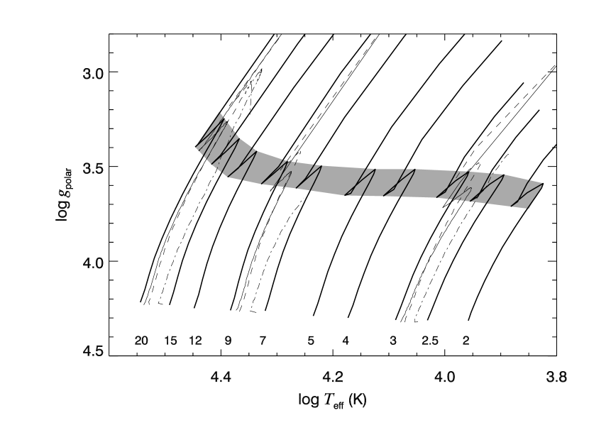
Figure 2: A comparison of the evolutionary tracks for non-rotating stellar models by Schaller et al. (1992) (thick solid lines) and for rotating models by Ekström et al. (2008) (thin lines: $\Omega/\Omega_{\rm crit}=0.1$; dashed lines: $\Omega/\Omega_{\rm crit}=0.5$; dash-dotted lines: $\Omega/\Omega_{\rm crit}=0.9$). The masses of the rotating models are 20, 9, and 3 $M_{\odot}$ from left to right, respectively. The masses (in $M_{\odot}$) of non-rotating models are marked by the numbers at the bottom.

We can approximately derive the stellar mass by assuming that the star follows a non-rotating star evolutionary track (Schaller et al., 1992) in the $(T_{\rm eff},\log g)$ plane with a current position at $(T_{\rm eff},\log g_{\rm polar}$). Here we assume that our derived hemisphere average $T_{\rm eff}$ is a reasonable choice for the whole surface average $T_{\rm eff}$. Any differences between model tracks for rotating and non-rotating stars will clearly influence the resulting mass estimate. We plot the evolutionary tracks for both non-rotating (Schaller et al., 1992) and rotating (Ekström et al., 2008) models in Figure 1. This comparison shows that the differences are minimal between the slow ($\Omega/\Omega_{\rm crit}=0.1$) and moderately fast ($\Omega/\Omega_{\rm crit}=0.5$) rotating models, while the evolutionary tracks of the very rapidly rotating models ($\Omega/\Omega_{\rm crit}=0.9$) are shifted to lower temperature regions occupied by the lower mass, non-rotating models. Our method may lead to a systematic underestimation of stellar mass by about 10% for such rapid rotators. Note that there is a significant shift in effective temperature between the non-rotating and slow rotating ($\Omega/\Omega_{\rm crit}=0.1$) tracks for a given mass that indicates that there are systematic model differences unrelated to rotation. One other error source for the estimated mass is related to the placement in the “zig-zag” portion of the evolutionary tracks that corresponds to the terminal age main sequence (TAMS; gray area in Fig. 2). Since stars spend more time on the cooler portion of the track compared to the hotter, advanced stage of evolution, we decided to use the low temperature segment of the tracks in the shadowed area to determine stellar mass. The derived mass values of those more evolved stars in this region could be overestimated by up to 10%, although the percentage of such stars is expected to be low.

Once we estimate stellar mass, we can derive the polar radius ($r_{\rm p}$), and then calculate the critical rotational velocity using the formula for the simple Roche model (point-source gravitational plus rotational potential fields),

$$V_{\rm crit}=\sqrt{\frac{2}{3}\frac{GM}{r_{\rm p}}}.$$ (1)

Here we can see how the mass errors propagate into $V_{\rm crit}$ errors. If mass were overestimated by 10%, then $r_{\rm p}$ would be overestimated by 5% (from $\log g_{\rm polar}$), and $V_{\rm crit}$ would be overestimated by only 2.5%. Thus, the errors in mass described in the previous paragraph will result in relative errors in $V_{\rm crit}$ of $<2.5\%$.

The final derived parameters of our newly measured sample B stars are given in Table 3 (cluster stars) and Table 4 (field stars) whose full contents are available only in the electric form. Table 3 lists the cluster name, stellar identification number from WEBDA, radial velocities, $V\sin i$, and the derived physical parameters. The heliocentric Julian dates (HJD) of observation are given for each cluster in the electronic table header. Table 4 lists the star identifications in the SAO and Henry Draper (HD) catalogs, HJD of observation, and then the other quantities as in Table 3. The total numbers of B stars in our complete sample are summarized in Table 5 according to cluster or field membership and radial velocity variability status. Combining both new (first two rows in Table 5) and prior data (last two rows in Table 5) gives us a large and homogeneous sample ($\approx 1000$ stars) for the statistical analyses presented in following sections.

4 Field and Cluster Star Rotation Properties

We argued above that the rotational properties of binary stars may not be representative of B-stars as a whole, and so we set aside the subsample of radial velocity variable stars (probably binaries). The next issue to resolve is whether B stars in the field and in clusters have such different rotational properties that the results for stars in the two categories need to be analyzed separately. Both Abt et al. (2002) and Huang & Gies (2006a) found that nearby field B stars appear to rotate slower on average than B stars in young open clusters. The authors argue that this difference results from evolutionary spin-down with time and the relatively greater age of the field stars. The same systematic difference in rotation rates was also demonstrated in a series of papers by Strom et al. (2005) and Wolff et al. (2007, 2008). These authors argue instead that the trend results from the variation in density of the birthplace environment. To settle this issue, we recently presented an analysis of spectra of 108 field B stars (Huang & Gies, 2008) that was done in the same way as our earlier cluster study (Huang & Gies, 2006b). This work showed that both the field and cluster stars exhibit a similar spin-down with advanced evolution (when the stars are grouped into common $\log g_{\rm polar}$ bins) and that field stars are generally more evolved than the those in clusters. Here we repeat this comparison strategy with much larger samples.

The fact that, on average, cluster B stars rotate faster than field B stars is clearly confirmed again with our new B star samples. We show in Figure 3 the cumulative distribution functions of $V\sin i$ for the total samples of 419 field and 524 cluster stars (all constant velocity stars). The mean $V\sin i$ is $110.7\pm 4.6$ km s^-1 for the field sample and $145.2\pm 4.1$ km s^-1 for the cluster sample. A Kolmogorov-Smirnov (K-S) test shows that there is a very low probability ($2\times 10^{-10}$) that the two samples are drawn from the same population.

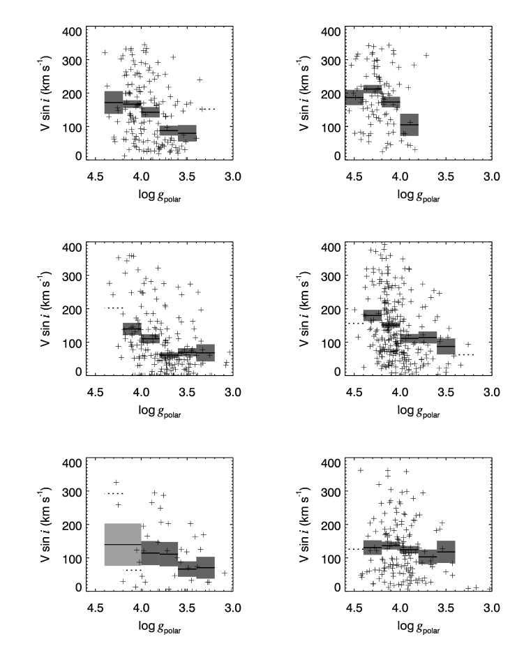
Figure 5: Scatter plots of $V\sin i$ as a function of $\log g_{\rm polar}$ for the field (left column) and cluster samples (right column) and for three mass ranges: $2<M/M_{\odot}<4$ (top), $4\leq M/M_{\odot}<8$ (middle), and $M/M_{\odot}\geq 8$ (bottom). The solid horizontal lines indicate the mean $V\sin i$ of each bin containing six or more stars while dotted lines indicate the same for the bins containing fewer. Shaded areas illustrate the standard deviation of the mean for each bin.

If we plot the $\log g_{\rm polar}$ histogram for both the cluster and field B stars (Fig. 4), we can clearly see the difference in evolutionary state of the two samples: the field B sample contains more stars with lower $\log g_{\rm polar}$. The mean $\log g_{\rm polar}$ is 3.80 for the field B star sample and is 4.11 for the cluster sample. Therefore, we suggest that the slower rotation of our field sample is due solely to the greater influence of evolutionary spin down in a relatively older population. This can be demonstrated by constructing diagrams of mean $V\sin i$ as a function of $\log g_{\rm polar}$ for different mass groups among both the field and cluster B stars. We show such plots in Figure 5 for the field (left) and cluster stars (right) for three mass groups: a low mass group ($2<M/M_{\odot}<4$; top), a moderate mass group ($4<M/M_{\odot}<8$; middle), and a high mass group ($M/M_{\odot}>8$; bottom). For each mass group, we calculate the mean of $V\sin i$ for stars that are binned according to $\log g_{\rm polar}$ (over a range of 0.2 dex for each bin). Note that since there are only six young ($\log g_{\rm polar}>4.0$) field stars in the high mass subgroup, we consolidate two high $\log g_{\rm polar}$ bins into one as shown in Figure 5. If the bin contains data for six or more stars, then we also calculate the standard deviation of the mean (shown as shaded areas in Figure 5). We find that the evolutionary spin down trend is present in all subgroups of both the field and cluster samples (although with shallower slope among the more massive stars). The results are also in qualitative agreement with those of Abt et al. (2002) and Abt (2003) who examined a similar number of B stars and found that between luminosity class V (unevolved) and class III (evolved) the mean projected rotational velocity declines by $\approx 15\%$ for early-B types and by $\approx 40\%$ for late-B types. If we compare the individual bins of the field stars with the corresponding ones of the cluster stars, we find that all of the matched pairs have similar mean $V\sin i$ (within one standard deviation) except for one set with $3.6<\log g_{\rm polar}<3.8$ in the mid-mass subgroup. Note, however, that the number of field B stars in the high mass group ($>8M_{\odot}$) is small (a total of only 46 field B stars), and a larger sample would help establish the details of the spin-down for this group. These results are very similar to our previous findings (Huang & Gies, 2008) which were based on a smaller sample of field stars. Thus, since the spin-down trends appear to be similar in the field and cluster stars and since the field stars tend to be more evolved (lower $\log g_{\rm polar}$), we again conclude that the lower rotation rates of the field stars are primarily the result of evolutionary spin-down changes.

In contrast to our results, Wolff et al. (2007) did not detect a significant evolutionary change in stellar rotation among their sample of stars, and they concluded that differences in initial conditions and mass densities of star forming regions are key to explaining the differences in rotational properties. Wolff et al. (2007) compared rotational properties of B0 – B3 stars (correponding to an approximate mass range of $6-12M_{\odot}$) in young and old clusters and associations in both low density ($\rho<1M_{\odot}~{}{\rm pc}^{-3}$) and high density ($\rho>1M_{\odot}~{}{\rm pc}^{-3}$) environments. They found that a small spin-down was evident when comparing the cumulative distribution functions of $V\sin i$ for young and old dense clusters (see their Fig. 3). This relatively small spin-down rate probably results in part because their sample consists mainly of more massive B-stars and because the spin-down rates may be slower (as a function of $\log g_{\rm polar}$) among massive B stars (see Fig. 5). Furthermore, some of the spin-down trend may be lost when samples are binned according to cluster age. The time scale of interest for evolutionary changes is the main sequence lifetime, which depends sensitively on stellar mass, $\tau_{\rm MS}\propto M^{-2}$. According to Schaller et al. (1992), a $6M_{\odot}$ star has $\tau_{\rm MS}=63$ Myr while a $12M_{\odot}$ star has $\tau_{\rm MS}=16$ Myr. Thus, while the young age group of cluster stars (1 – 6 Myr) considered by Wolff et al. consists of mainly unevolved stars, the group of older cluster stars (11 – 16 Myr) probably includes some evolved massive stars ($69-100\%~{}\tau_{\rm MS}$ for $M=12M_{\odot}$) and many unevolved, lower mass stars ($17-25\%~{}\tau_{\rm MS}$ for $M=6M_{\odot}$). Thus, depending on the mass distribution of stars, the rotational properties of the older group may show little or no evidence of evolutionary spin-down because of the mixture of evolutionary states represented within the sample.

Wolff et al. (2007) found much larger differences in the rotational properties between stars in high and low density environments. By their criterion, all the cluster stars that we observed will belong to the high density group (and all the field stars to the low density group). We estimated cluster densities (for both the clusters listed in Table 1 and those observed earlier that are listed in Table 4 of Huang & Gies 2006a) from the total masses derived by Piskunov et al. (2008; their $\log M_{\rm A}$) and from the cluster angular radii and distances from Kharchenko et al. (2005; using their $R_{\rm core}$). We have five clusters in common with the sample from Wolff et al.: NGC 869, 884, 2244, 7380, and IC 1805. The density comparison is difficult for NGC 869 and 884 because these clusters overlap in the sky, and their $\log M_{\rm A}$ values are overestimated (Piskunov et al., 2008). For NGC 2244, 7380, and IC 1805, the derived mass densities are 5, 18, and 15 $M_{\odot}$ pc^-3, respectively, which are comparable to the corresponding results of 11, 5, and 10 $M_{\odot}$ pc^-3 derived by Wolff et al. (2007) using somewhat different assumptions. The mass density range of our sample of clusters runs from 1 to 78 $M_{\odot}$ pc^-3 (and higher for NGC 869 and 884), and, thus, all the clusters we observed belong to the high density category defined by Wolff et al. (2007). However, the distributions of $V\sin i$ in our high (cluster) and low density (field) samples show no evidence of systematic differences when binned according to polar gravity (see Fig. 5). To make as best a comparison as possible with the mass range considered by Wolff et al., we selected a subset of stars in the mass range $6-12M_{\odot}$ and determined the rotational properties as a function of polar gravity. The results (summarized in Table 6) indicate that there are no significant differences (within the statistical errors) between the field and cluster mean values. Our results do not rule out the role of environmental factors (especially among the more massive B-stars where our sample contains fewer targets), but given that there is no evidence of systematic differences between the cluster and field stars within our sample, we will consider the combined set of field and cluster stars together in the following sections.

5 Young Main Sequence B Stars

When we study stellar rotation and its evolution, there is one key aspect that we want to glean from observations. That is how fast stars rotate when they just start off their main sequence journey at the ZAMS. These initial rates are important because they show us how fast stars rotate at one of the most important moments in their lifetime, ZAMS, representing both the starting point of the relatively simple (smoothly changing) MS stage and the end point of the extremely complicated pre-MS stage. Accurate stellar rotation data at the ZAMS can help us to understand the role of angular momentum in stellar evolution both before and after the ZAMS (cf. Wolff et al. 2004). Theoretically, the ZAMS only defines a moment when hydrogen fusion is ignited in the stellar core (the temporal boundary between “protostar” and “star”). The evolutionary change of stellar rotation after ZAMS is expected to be smooth and slow. Thus, by studying the rotational properties of the least evolved B stars in our single ($V_{\rm r}$ constant) star sample, we should be able to obtain a reliable picture about how fast the ZAMS stars rotate. Since the ZAMS line of theoretical stellar models in the mass range of B stars has basically the same surface gravity ($\log g\sim 4.2$; see Fig. 2), we decided to select all single B stars with $\log g_{\rm polar}>4.15$ to form a subsample that we will call the Young Main Sequence (YMS) stars.

We have a total of 220 B stars in our YMS sample. The stellar rotation distribution of $V\sin i/V_{\rm crit}$ for the entire YMS sample is shown in Figure 6. We made a simple polynomial fit of the histogram data of $V\sin i/V_{\rm crit}$ (thin line), and then we used the deconvolution algorithm from Lucy (1974) to derive the distribution of $V_{\rm eq}/V_{\rm crit}$ (thick line). Figure 6 indicates that B stars in our sample are born with various rotation rates. The highest probability density occurs around $V_{\rm eq}/V_{\rm crit}=0.49$. About 6% of newborn B stars are very slow rotators ($V_{\rm eq}/V_{\rm crit}<0.1$), while about 52% of the B stars are born with a value of $V_{\rm eq}/V_{\rm crit}$ between 0.4 and 0.8. Only 1.3% of B stars are born as very rapid rotators ($V_{\rm eq}/V_{\rm crit}>0.9$). Wolff et al. (2004) have already shown from their data that the specific angular momentum of very young B stars is spread well below the critical limit. Now we can see this more clearly in quantitative form in the $V_{\rm eq}/V_{\rm crit}$ distribution curve.

To investigate if these statistical data depend on stellar mass, we divided our YMS sample into three subgroups: low mass ($2\leq M/M_{\odot}<4$; 90 stars), middle mass ($4\leq M/M_{\odot}<8$; 92 stars), and high mass ($M/M_{\odot}\geq 8$; 38 stars). We would expect to see distribution curves similar to that in Figure 6 if YMS B stars in the different mass subgroups were born with a similar spin rate distribution. However, as shown in Figure 7, the statistics clearly reveal a different story: as stellar mass increases, more and more stars are born as slow rotators (with lower $V_{\rm eq}/V_{\rm crit}$ values). The fraction of slow rotators (say, $V_{\rm eq}/V_{\rm crit}<0.5$) in each subgroup are 37%, 53%, and 84% for the low, middle, and high mass subgroup, respectively.

The statistical results on the stellar rotation rates of the YMS B stars present some very interesting findings: 1) Even if we generally accept that most massive stars are born as rapid rotators, there does exist a significant fraction of newborn B stars that are very slow rotators (e.g., $V_{\rm eq}/V_{\rm crit}<0.1$). There must exist some processes that efficiently brake these slow rotators early on. 2) Compared to the less massive stars, the more massive stars tend to be born as slow rotators. Qualitatively, two factors may contribute to this. First, we know that stronger stellar winds occur in more massive stars, and these can effectively remove angular momentum (Meynet & Maeder, 2000). Secondly, we know that the binary frequency is high among the massive O-stars (Mason et al., 2009). It may be that star formation processes may tend to deposit angular momentum more in orbital motion and less in stellar spin among the more massive stars (Larson, 2007, 2010). Abt (2009), for example, found that stars in dense environments (usually where more massive stars are found) tend to have more binary systems and lower mean $V\sin i$ values.

6 Rotational Upper Limits and Be Stars

As discussed by Porter & Rivinius (2003), the “Be” phenomenon is associated with a wide range of B stars whose spectra have exhibited emission features in the Balmer line regions at some point in time. We focus here on the so-called classical Be stars, non-supergiant B stars whose spectra generally show broad, photospheric, absorption lines that are indicative of fast rotation. To form a gaseous disk around a star and generate the emission features, it is generally thought that the star has to rotate very fast so that the centrifugal force significantly cancels the gravitational force and makes it relatively easy to launch gas into orbit. How fast can a B star spin before it becomes a Be star? This is a controversial topic in the recent literature on Be stars, and the fact that there is still no widely accepted answer is partially due to the difficulty of obtaining reliable $V_{\rm eq}$ estimates for Be stars. Because we can only derive $V\sin i$ from observational data, we require measurements of a large sample of Be stars to deal with the $\sin i$ factor in a statistical way. Yudin (2001) carried out a large rotation survey of Be stars and, by assigning $V_{\rm crit}$ to each spectral subtype, he obtained values of $<V_{\rm eq}>/<V_{\rm crit}>$ ranging from 0.5 to 0.8. Porter (1996) investigated some Be-shell stars which are presumably edge-on Be stars ($\sin i\sim 1$), and his result suggests that the Be stars, if not different from his Be-shell star sample, should rotate at 70$\sim$80% of $V_{\rm crit}$. This range was confirmed by the study of Be stars in the open cluster NGC 3766 by McSwain et al. (2008), who compared the observational $V\sin i$ cumulative distribution function with the theoretical one. However, Townsend et al. (2004) point out that very rapidly rotating stars may experience strong gravitational darkening towards their equatorial zones that leads to an underestimate of the actual $V\sin i$ value. They applied a correction for this effect to the data available from Chauville et al. (2001), and their results imply that Be stars are spinning close to the critical rotation rate. On the other hand, some later studies that took the gravitational darkening effect into account (Frémat et al., 2005; Cranmer, 2005) still favored relatively low $V_{\rm eq}/V_{\rm crit}$ values for Be stars. Howarth (2007) points out that the high $V_{\rm eq}/V_{\rm crit}$ ratio (0.95 or higher) case only requires “weak” processes to lift the surface material into orbit, while the low ratio case needs much more energy to send gas into orbit (the velocity gap between surface and orbit can reach as much as 100 km s^-1 in this case). He suggests that, if Be stars can form in the low ratio situation, the signatures of “strong” processes in stellar photosphere (such as “large-amplitude pulsations”) should be easily detected. More recently, Cranmer (2009) developed a detailed theoretical pulsational model that suggests that a Keplerian disk could form around Be stars with $V_{\rm eq}/V_{\rm crit}$ as low as 0.6.

Although our survey was focused primarily on the rotational properties of normal B stars, we can use our sample to investigate this issue by considering the upper limit of $V_{\rm eq}/V_{\rm crit}$ for those stars that probably are rotating at rates slightly below that required to form a Be disk. To achieve this goal, we first removed all the Be stars from our single ($V_{\rm r}$ constant) star sample by excluding already known Be stars and those with Balmer emission or deep, narrow, absorption lines (a signature of Be-shell stars) in our spectra. This process led to a culling of 61 Be stars, leaving a total of 894 stars in the remaining sample (presumably all non-emission line B stars). These Be stars are identified in the last column of Tables 3 and 4. Note that our approach here makes the tacit assumption that the processes leading to disk formation require a certain minimum value of the ratio of equatorial velocity to critical rotation. Ideally, we could test this idea by finding a minimum value of this ratio among the Be stars, but unfortunately, it is difficult to apply our methods to Be stars because of emission contamination in the profiles and the small number of Be stars we observed. Instead, we will simply compare below our results on the fastest rotating, non-emission line stars with results on the Be stars from other investigations. Since the process of disk formation probably requires rapid rotation and some other mechanical energy source (possibly pulsation; Rivinius et al., 2003; Cranmer, 2009) and since the properties of the latter may vary from star to star, we caution that the $V_{\rm eq}/V_{\rm crit}$ criterion for disk formation will probably apply only in some average sense.

We can approach the problem of finding a nominal upper limit on $V_{\rm eq}/V_{\rm crit}$ in two ways. First, we can consider the observed upper limit in the distribution of $V\sin i/V_{\rm crit}$. One could simply adopt the largest derived value of this ratio as the upper limit for $V_{\rm eq}/V_{\rm crit}$, but because the errors associated with any given estimate are not negligible, we prefer to form a mean from a subset of stars with the largest observed ratios. Clearly, the larger the sample, the more well defined will be the upper limit boundary of the distribution. Those stars that help us set the upper limit will have a $V_{\rm eq}/V_{\rm crit}$ ratio close to the limit and will have an inclination angle close to 90^∘ (i.e., $\sin i\approx 1$). If we choose the top 4% of stars that have the highest $V_{\rm eq}/V_{\rm crit}$ values (the fastest rotators) and assume that their spin axes are randomly pointed in space, then about $1/4$ of these stars will have $\sin i>0.97$. Thus, we expect that those stars in the top 1% of the $V\sin i/V_{\rm crit}$ distribution probably correspond to very fast rotators (in the top 4%) with an edge-on orientation ($\sin i>0.97$). Therefore, for our sample of about 900 stars, the mean ratio from the top nine fast rotators of $V\sin i/V_{\rm crit}=0.91$ provides an initial estimate of the limit separating the non-emission line and emission-line stars. We list in the lower row of Table 7 this estimate plus the unique maximum and 3% subsample estimates for the upper limit from all the $V\sin i/V_{\rm crit}$ measurements.

A second approach is to use the deconvolution method of Lucy (1974) to derive the $V_{\rm eq}/V_{\rm crit}$ distribution from the $V\sin i/V_{\rm crit}$ distribution (as shown earlier in Fig. 6 and 7), and then determine the value of $V_{\rm eq}/V_{\rm crit}$ that marks the boundary for a given percentage of the distribution. The final row of Table 7 gives these boundaries for the top 4% and 0.2% of the reconstructed $V_{\rm eq}/V_{\rm crit}$ distribution for the full sample of non-emission line stars. The fact that the 4% boundary ratio ($V_{\rm eq}/V_{\rm crit}=0.88$) is quite similar to the estimate from the top 1% of the $V\sin i/V_{\rm crit}$ distribution ($<V\sin i/V_{\rm crit}>_{\rm 1\%}=0.91$) indicates that both methods leads to similar and presumably reliable results.

However, we found in §5 that the rotational properties of the youngest B stars in our sample are strongly dependent upon the mass subgroup (slower among the more massive stars; see Fig. 7), and thus, it is important to consider the upper limit of $V_{\rm eq}/V_{\rm crit}$ among samples of comparable mass. In order to obtain meaningful results from each mass subsample, we need to keep the population large enough so that 1% of their content comprises at least 2 stars. Thus, we divided our total of 894 stars into four subsamples based upon mass. The mass range of each subsample is given in the first column of Table 7. We made the same two statistical estimates for the upper limit of $V_{\rm eq}/V_{\rm crit}$ for each subsample. All the key statistical results are given in columns (2) to (7) of Table 7. The estimates based on the maximum value (from one star; column 3) and the mean value of $<V\sin i/V_{\rm crit}>$ for the top 1% of the stars (based on 2–3 stars; column 4) suffer from small number statistical errors. Instead, estimates from $<V\sin i/V_{\rm crit}>$ of the top 3% of stars (5–8 stars; column 5) and from the boundary of $V_{\rm eq}/V_{\rm crit}$ for the top 4% of the rapid rotators (6–10 stars; column 6) provide more reliable results.

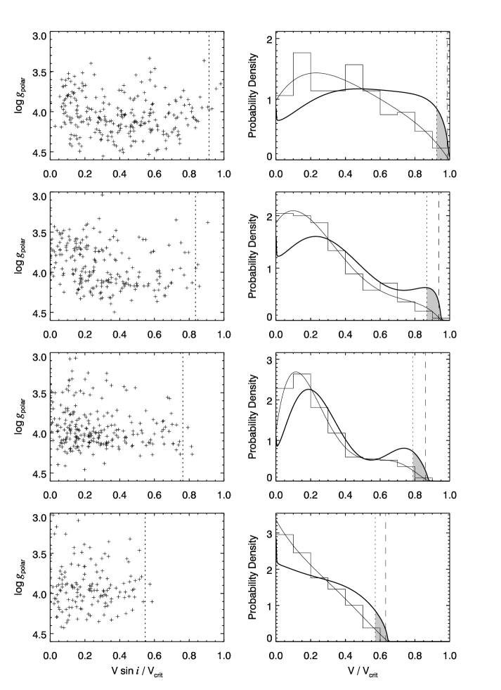
Figure 8: Scatter plots of $(V\sin i/V_{\rm crit},\log g_{\rm polar})$ and rotational distributions (in the same format as Fig. 7) for non-emission line stars. From top to bottom, each pair corresponds to mass ranges of $2.2\leq M/M_{\odot}<4.0$, $4.0\leq M/M_{\odot}<5.4$, $5.4\leq M/M_{\odot}<8.6$, and $M/M_{\odot}\geq 8.6$. The shaded areas indicate the top 4% stars in the $V_{\rm eq}/V_{\rm crit}$ distributions.

We illustrate the rotational properties of the fastest spinning, non-emission line stars in two sets of panels in Figure 8. The left hand panels show the distributions in the $(V\sin i/V_{\rm crit}$, $\log g_{\rm polar})$ plane with a dotted line marking the mean $<V\sin i/V_{\rm crit}>$ of the top 3% of stars, while the right hand panels show the histograms of $V\sin i/V_{\rm crit}$ and the deconvolved functions $V_{\rm eq}/V_{\rm crit}$ (format similar to Fig. 6 and 7). The dotted and dashed lines in the right hand panels indicate the boundaries in the $V_{\rm eq}/V_{\rm crit}$ distribution for the top 4% and 0.2% of the sample, respectively. These panels are arranged in four rows corresponding to the four mass subgroups (from low mass at the top to high mass at the bottom).

We can immediately see from Figure 8 that the rotational upper limit for non-emission line B stars does indeed depend on stellar mass. Estimates of the upper limit from both $<V\sin i/V_{\rm crit}>_{\rm 3\%}$ and $(V_{\rm eq}/V_{\rm crit})_{\rm 4\%}$ show a consistent drop from about 0.92 in the $3M_{\odot}$ subsample to about 0.56 in the $9M_{\odot}$ group. In principle, we might take the rotational upper limit as the value of $V_{\rm eq}/V_{\rm crit}$ where the deconvolved function reaches zero probability in Figure 8. However, the detailed shape of this function at the top end depends critically on the small numbers in the last few populated bins of $V\sin i/V_{\rm crit}$. Thus, we arbitrarily adopted upper limit as the boundary of $V_{\rm eq}/V_{\rm crit}$ for the top 0.2% of the deconvolved distribution, since this value is somewhat better constrained and corresponds to the case where we might find 0 or 1 star in our subsamples. It is hard to estimate the error bars of the adopted upper limit of $V_{\rm eq}/V_{\rm crit}$ from regular methods. However, since the $<V\sin i/V_{\rm crit}>_{3\%}$ and $(V_{\rm eq}/V_{\rm crit})_{4\%}$ statistical values in Table 7 are quite reliable and comparable, their mean can can serve as the lower boundary to the upper limit of $V_{\rm eq}/V_{\rm crit}$. Then a working estimate of the error in the upper limit can be formed by taking the difference between $(V_{\rm eq}/V_{\rm crit})_{\rm 0.2\%}$ and the mean of $<V\sin i/V_{\rm crit}>_{\rm 3\%}$ and $(V_{\rm eq}/V_{\rm crit})_{\rm 4\%}$. Our final estimates of the rotational upper limits are given in column 7 of Table 7.

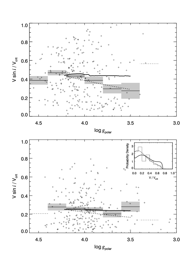
Figure 10: The $V\sin i/V_{\rm crit}$ vs. $\log g_{\rm polar}$ plots for B stars in mass range $2<M/M_{\odot}<4$ (top panel) and in the range $7\leq M/M_{\odot}<13$ (bottom panel), using the same format as in Fig. 5. The thick curves are theoretical predictions based on $3M_{\odot}$ (top panel) and 9 $M_{\odot}$ (bottom panel) models from Ekström et al. (2008). The predictions of the case B model are plotted as thick dotted lines. The embedded plot in the bottom panel shows the rotation distribution curves for the YMS stars with $7\leq M/M_{\odot}<13$ (same format as Fig. 6).

These results suggest that the rotational threshold required to create a Be star disk varies dramatically through the B star mass range. For example, we find that low mass B stars ($M<4M_{\odot}$, or spectral subtype later than B6 for MS stars) may rotate extremely fast ($V_{\rm eq}/V_{\rm crit}\sim 0.96$) without creating an outflowing disk. This may explain why the fast rotator, Regulus (below the threshold at $V_{\rm eq}/V_{\rm crit}=0.86$; McAlister et al. 2005), has never exhibited any Balmer line emission. For stellar masses $>8.6M_{\odot}$ (spectral subtype B2 or earlier for MS stars), the threshold drops to $V_{\rm eq}/V_{\rm crit}\sim 0.63$. This result may help resolve the controversy surrounding the massive Be star, Achernar ($\sim 7M_{\odot}$). Interferometric observations of Achernar by Domiciano de Souza et al. (2003) showed that the star has an exceptionally large rotational oblateness with $R_{\rm eq}/R_{\rm polar}=1.56$, which is above the value expected (1.5) for a star rotating at the critical rate. However, a recent spectroscopic analysis by Vinicius et al. (2006) indicates that Achernar may rotate at $\Omega/\Omega_{\rm crit}\sim 0.8$, which is equivalent to $V_{\rm eq}/V_{\rm crit}\sim 0.65$ (cf. Fig. 10 in Ekström et al. 2008). Note that this rate is probably near to the implied threshold we find for disk formation among the massive B stars, so Achernar’s rotation rate and status as a Be star are probably consistent with our results.

The mass dependence of the rotation limit was generally ignored in past with the notable exception of Cranmer (2005) who reported a very similar $V_{\rm eq}/V_{\rm crit}$ dependence on spectral-type. He applied Monte Carlo forward modeling to a sample of 462 classical Be stars to test various $V_{\rm eq}/V_{\rm crit}$ distribution functions against the observed $V\sin i/V_{\rm crit}$ distribution. His conclusion was that hot B stars ($T_{\rm eff}\gtrsim 21000$K) tend to have a low threshold of $V_{\rm eq}/V_{\rm crit}$ (“well below unity”) while cool B stars ($T_{\rm eff}\lesssim 21000$K) have an increasing threshold of $V_{\rm eq}/V_{\rm crit}$ (up to unity) as “$T_{\rm eff}$ decreases to the end of the B spectral range”. Howarth (2007) raised two concerns about these results: 1) they were based on very heterogeneous data sources, and 2) $V_{\rm crit}$ was assigned to individual stars according to spectral type. However, these concerns do not apply to our sample, and the overall good agreement between our result (based on normal B stars) and Cranmer’s (based on classical Be stars) convinces us that the rotational limit for Be star formation is indeed mass dependent.

We should note that most of the B stars in our sample were retained for this analysis based upon an examination of only a few spectra for Balmer line emission. However, Be stars are intrinsically variable in nature (Porter & Rivinius, 2003), and in some cases (“transient Be stars”) the disk emission may even disappear at times (cf. McSwain et al. 2009). It is possible that some of the fast rotators used in our analysis are transient Be stars that we observed during an emission-free epoch. If such Be stars do exist among those high $V\sin i/V_{\rm crit}$ stars that we used to determine the rotational upper limit, then we may have overestimated the limits. We list in Table 8 all the stars with high $V\sin i/V_{\rm crit}$ that helped define our derived upper limits, and we recommend spectroscopic H$\alpha$ monitoring of these targets to verify their status as normal (non-emission line) B stars.

7 Rotational Evolution of Main Sequence B Stars

Theoretical studies (Heger & Langer, 2000; Meynet & Maeder, 2000) demonstrate that the evolutionary paths of rapidly rotating, massive stars can be very different from those for non-rotating stars. Rapid rotation can trigger strong interior mixing, extend the core hydrogen-burning lifetime, significantly alter the luminosity, and change the chemical composition of the outer layers over time. The most detailed models to date are presented in a seminal paper by Ekström et al. (2008) (=EMMB), who show how the equatorial velocities and surface abundances change with time according to the initial rotation rate, metallicity, and mass. We have already shown in §4 (Fig. 5) that the mean rotational properties do vary with $\log g_{\rm polar}$, our measurement of evolutionary state. In this section, we re-sample our rotational data into two mass categories from the EMMB model grid, and we compare the observed changes with $\log g_{\rm polar}$ to predictions from the EMMB models that are based upon an initial rotational distribution derived from the youngest MS stars.

Our goal is to compare our rotational results with the EMMB models for solar metallicity (a reasonable assumption for nearby, Galactic, B stars). The EMMB models are presented for masses of 3, 9, 20, and $60M_{\odot}$, and since massive stars with $M>15M_{\odot}$ are sparse in our sample, we are limited to making the comparison with the EMMB models for $3M_{\odot}$ and $9M_{\odot}$. We selected stars with $2\leq M/M_{\odot}<4$ (262 stars; $<M>=3.2M_{\odot}$) for the $3M_{\odot}$ group and those with $7\leq M/M_{\odot}<13$ (241 stars; $<M>=9.2M_{\odot}$) for the $9M_{\odot}$ group. All the known and suspected Be stars were omitted from these samples because we cannot derive reliable $T_{\rm eff}$ and $\log g$ parameters from the emission-blended H$\gamma$ profile. For each group, we first derived the rotational distribution curve (probability density vs. $V_{\rm eq}/V_{\rm crit}$) of the YMS stars ($\log g_{\rm polar}>4.15$; 90 stars in the 3 $M_{\odot}$ group, and 49 stars in the 9 $M_{\odot}$ group) using the same method described in §5. These functions describe the initial distribution of $V_{\rm eq}/V_{\rm crit}$. Then the EMMB theoretical models can be used to show how these distributions should change with time and, consequently, how $<V\sin i/V_{\rm crit}>$ should change with time. This mean ratio can be directly compared to our observational results as a function of $\log g_{\rm polar}$ to investigate evolutionary changes.

The EMMB models provide the key data on how stellar rotation evolves with time for initial (ZAMS) values of angular rotational rate $\Omega/\Omega_{\rm crit}=$ 0.1, 0.3, 0.5, 0.7, 0.8, 0.9, and 0.99. Figure 9 shows how the $V_{\rm eq}/V_{\rm crit}$ ratio changes with $\log g_{\rm polar}$ in the models for each of these starting rotational rates. We see that the EMMB models predict that a sharp drop occurs at the outset for stars with higher initial $V_{\rm eq}/V_{\rm crit}$ values. This results from a rapid redistribution of angular momentum as the models transform from an assumed solid body rotation state at ZAMS into a differentially rotating configuration. Our YMS star sample is best compared to the models that have stabilized and that are characterized by a mean $\log g_{\rm polar}$ similar to that of our YMS samples. Thus, we adopted $\log g_{\rm polar}=4.22$ as the nominal starting point for the model calculations. Then the deconvolved distribution of $V_{\rm eq}/V_{\rm crit}$ derived from the YMS stars maps into a probability density for each of the EMMB tracks shown in Figure 9. Note, however, that at this stage of evolution ($\log g_{\rm polar}=4.22$), the EMMB tracks only sample a range from $V_{\rm eq}/V_{\rm crit}=0.0$ to 0.7, and we need to extrapolate beyond these tracks for the portion of the rotational distribution with the fastest spins.

We then performed a numerical integration in small steps of $\triangle\log g_{\rm polar}$ to find how the probability becomes redistributed in $V_{\rm eq}/V_{\rm crit}$ as evolution advances. From inspection of Figure 9, the part of the distribution for the slowly spinning stars will be shifted only slightly higher, while the portions of the distribution for the fastest rotators will be shifted to significantly higher $V_{\rm eq}/V_{\rm crit}$. Ekström et al. (2008) argue that these rapidly rotating stars will evolve towards the critical limit, where they may become Be stars and drain their angular momentum into a circumstellar disk. However, we purposely removed the Be stars from our observational sample, so we need to truncate the fastest portion of the evolved model distributions of $V_{\rm eq}/V_{\rm crit}$ in order to make a valid comparison with the observed distributions. From our results in §6 (see Table 7), we estimate that the upper limit boundary separating the non-emission line and Be stars occurs near $V_{\rm eq}/V_{\rm crit}=0.96$ for a $3M_{\odot}$ star and near $V_{\rm eq}/V_{\rm crit}=0.75$ for a $9M_{\odot}$ star. These limits are indicated by dotted, horizontal lines in Figure 9. Thus, we treated any part of the model $V_{\rm eq}/V_{\rm crit}$ distribution that was transformed above these limits as removed from the sample. We then determined the mean value of $<V_{\rm eq}/V_{\rm crit}>$ from the remaining model distribution at each increment of $\log g_{\rm polar}$ (over the range $4.22>\log g_{\rm polar}>3.5$; indicated by vertical dotted lines in Fig. 9). Finally, this statistic was multiplied by $\pi/4$ (assuming random orientation) to obtain a model prediction of $<V\sin i/V_{\rm crit}>$. These calculated, mean rotational rates are plotted as thick solid lines in Figure 10 for the $3M_{\odot}$ and $9M_{\odot}$ cases, and the predictions suggest that the sample means should be almost constant over the main sequence lifetime. This may appear somewhat surprising, given the general trend of increasing $<V_{\rm eq}/V_{\rm crit}>$ for the tracks shown in Figure 9, but recall that the rapid rotators are systematically removed from the sample distribution once they exceed the nominal Be star boundary. This removal of the high end part of the distribution tends to cancel the effect of the small increase in $<V_{\rm eq}/V_{\rm crit}>$ for the lower velocity portion and results in almost no change in the distribution mean value.

We also show in Figure 10 the observed distributions of $V\sin i/V_{\rm crit}$ for the two mass samples. The mean values of $V\sin i/V_{\rm crit}$ of the observed stars in each 0.2 dex bin of $\log g_{\rm polar}$ are plotted as horizontal bars, and their associated standard deviations of the mean are shown as gray shaded regions (as in Fig. 5). The differences between the two mass groups are striking. The lower mass B stars (top panel of Fig. 10) rotate much faster than do the higher mass B stars (lower panel of Fig. 10) at the beginning of the MS stage, but the lower mass stars spin down much “faster” with respect to $\log g_{\rm polar}$ than do the higher mass stars. At the end of the MS stage, both low and high mass B stars have roughly the same $<V\sin i/V_{\rm crit}>$. Our results are in qualitative agreement with those of Abt et al. (2002) and Abt (2003) who examined a similar number of B stars and found that between luminosity class V (unevolved) and class III (evolved) the mean projected rotational velocity $<V\sin i>$ changes little for early-B types and drops significantly for late-B types.

A visual appraisal of the predicted and observed evolutionary trends indicates that the EMMB model prediction makes a good match of the observational results for the high mass, B star group but fails to reproduce the observed spin-down of the lower mass group. The evolutionary trends in the EMMB models are directly related to their formulation of the angular momentum redistribution in the stellar interior caused by mixing. The EMMB models occupy the middle ground between two extreme cases discussed by Oke & Greenstein (1954). In case A of Oke & Greenstein (1954), the angular momentum is fully fixed mixed within the interior and the star rotates as a solid body. As the star evolves with time, it becomes more concentrated towards its center (and its moment of inertia gradually decreases), and consequently the outer layers spin up in terms of $V_{\rm eq}/V_{\rm crit}$. Case B, on the other hand, imagines the star as a sequence of spherical mass shells in which each shell maintains its angular momentum. Then the surface rotational velocity will drop in proportion to the increase in radius with advanced evolution. Case A models, with their greater spin up, would tend to increase faster with advancing evolution than the EMMB models shown in Figure 10, while case B models, with more spin down, would decrease faster with advancing age. Since the observations suggest more spin down for the $3M_{\odot}$ group than predicted by the EMMB model, it is worthwhile considering the case B alternative.

In case B, we suppose that angular momentum is conserved in the individual spherical shells of a rotating star. Then, conservation of angular momentum in the outermost layer (where we measure $V\sin i$) directly leads to $V_{\rm eq}\propto r^{-1}$. Since $V_{\rm crit}\propto r^{-1/2}$, the ratio will vary as $V_{\rm eq}/V_{\rm crit}\propto r^{-1/2}\propto g_{\rm polar}^{1/4}$. The predicted trends of spin-down with $\log g_{\rm polar}$ for the case B model are plotted as dashed lines in Figure 9. Then we can calculate how the distributions of $V_{\rm eq}/V_{\rm crit}$ will change with advanced evolution according to the case B model and determine the mean $<V\sin i/V_{\rm crit}>$ in the same way as we did for the EMMB models. The case B model predictions are plotted as thick, dotted lines in Figure 10.

Surprisingly, the prediction from the simple case B model makes a good fit of the spin-down trend observed for the low mass group. For the high mass group, the fits from the case B and EMMB models are both reasonably good (except for the lowest gravity bin at $\log g_{\rm polar}\sim 3.5$ where the EMMB model fit is better). The small difference in the predictions between the EMMB and case B models is due to the placement of most of the high mass stars in the lower $V_{\rm eq}/V_{\rm crit}$ region (bottom inset panel of Fig. 10) where the evolutionary changes of both models are modest (see Fig. 9). Note that the case B model ignores any angular momentum loss from the surface caused by stellar winds. Such loss is negligible for the weak winds of the lower mass stars, but inclusion of the influence of the stronger winds of the higher mass stars would cause a somewhat larger spin-down than illustrated in Figure 10 and might result in a more discrepant fit.

We suspect that the failure of the EMMB models to match the faster spin-down we observe in the lower mass stars is related to missing physical processes that involve magnetism. The transport of internal angular momentum is a complex process that involves mixing, magnetic fields, and possibly gravity waves (Talon, 2008; Decressin et al., 2009). For example, Maeder et al. (2009) describe how differential rotation, meridional circulation, and mixing can generate a magnetic dynamo in some circumstances. The magnetic braking associated with the magnetic field and mass loss may then lead to a significant spin down of the star. We speculate that such magnetic braking is more apparent in the lower mass stars because their MS lifetimes are relatively much longer and consequently magnetic braking has a greater cumulative effect.

8 Consequences for Be Star Formation

Our results offer some insight about the evolutionary stages where we might expect to find the rapid rotation associated with disk formation in Be stars. There are three broad explanations for the origin of the rapid rotating Be stars: 1) they were born as rapid rotators; 2) angular momentum redistribution with evolution causes their outer layers to spin up (Ekström et al., 2008); and 3) they are the mass gainers that were spun up by a past episode of Roche lobe overflow in an interacting binary system (Pols et al., 1991). We showed in §5 that most young B stars have rotational velocities that are well below the limit for Be star formation (compare Fig. 7 for the YMS stars with Fig. 8 for the upper limits of non-emission line stars). Consequently, we think that only a small fraction of Be stars were born as rapid rotators, and below we will confront the expectations from the other two explanations with our results.

We showed in the last section (see Fig. 10, lower panel) that the EMMB model predictions about evolutionary changes in $<V\sin i/V_{\rm crit}>$ are consistent with the observed means for the higher mass stars. The EMMB models suggest that many of the stars in the upper part of the rotational distribution will evolve towards critical rotation (Fig. 9, lower panel) and presumably become Be stars. McSwain & Gies (2005) found that the Be fraction increases as high mass B stars evolve. Their data show that the Be fraction of early B stars is 4.7% while that of the evolved B stars increases to 7.4%. Zorec et al. (2005) also found that the Be star fraction increases between the early to late MS stages in Galactic stars in the mass range from 5 to $12M_{\odot}$, and Martayan et al. (2006) confirmed a similar trend for Be stars in the Large Magellanic Cloud (LMC). All these results are consistent with the EMMB picture that rapid rotation develops through the angular momentum redistribution that occurs as the stars approach the TAMS.

Using the EMMB model shown in the bottom panel of Figure 9 and our YMS data in the embedded portion of Figure 10, we can calculate how the Be fraction might change with time. According to the EMMB models, $V_{\rm eq}/V_{\rm crit}$ will generally increase with decreasing $\log g_{\rm polar}$, and once a star reaches the critical limit, it will remain there until the completion of core H burning. Suppose that a fraction $x$ of the sample are Be stars at the outset of the YMS star distribution (i.e., born as rapid rotators). Then, we can use the EMMB tracks to determine the number of high mass stars that should cross the Be formation limit as a function of evolutionary $\log g_{\rm polar}$. The calculation indicates that at $\log g_{\rm polar}=4.1$, the Be fraction is only about $x+3\%$ (formed from all the YMS B stars with $V_{\rm eq}/V_{\rm crit}>0.7$, see the embedded plot of Fig. 10); at $\log g_{\rm polar}=3.9$, the Be fraction increases to $x+12\%$ (from the YMS B stars with $V_{\rm eq}/V_{\rm crit}>0.6$); and at $\log g_{\rm polar}=3.6$, the Be fraction increases to $x+22\%$ (from the YMS B stars with $V_{\rm eq}/V_{\rm crit}>0.5$). This final estimate is in reasonable agreement with the results from McSwain & Gies (2005) (Be fraction for evolved B stars of $7.4\%$), given that the Be detection efficiency may be as low as 25 – 50% (McSwain et al., 2008).

However, the situation is different for the lower mass B stars. We found that the mean spin rates of the lower mass stars decrease faster than predicted by the EMMB model (Fig. 10, upper panel), which probably indicates that these stars evolve to lower $V_{\rm eq}/V_{\rm crit}$ (dashed lines in Fig. 9, upper panel). This conclusion is supported by the statistics of late type Be stars. If the EMMB models did apply to the lower mass B stars, then we can calculate the Be star fraction with time in the same way as we did above for the higher mass stars. Since the lower mass star distribution has a higher mean velocity, a larger proportion of the sample are predicted to end up as Be stars (see Fig. 9, upper panel). For example, all the low mass stars with $V_{\rm eq}/V_{\rm crit}>0.6$ at $\log g_{\rm polar}=4.22$ will be transformed into Be stars during the MS stage even though the boundary for Be formation is very high. According to the top panel of Fig. 7, about 45% of low mass YMS stars have $V_{\rm eq}/V_{\rm crit}>0.6$, and all of them are predicted to become Be stars before they reach the end of the MS stage. McSwain & Gies (2005) found that the Be fraction of the late B stars is only about 0.9%, which is much lower than the prediction from the EMMB model. Thus, the low observed Be fraction among the lower mass stars offers indirect evidence that these stars spin down faster than predicted.

This line of reasoning suggests that lower mass stars spin down with time. If this is also true of low mass Be stars, then any such star must be in a state where it obtained its high spin very recently, i.e., it is one of the rare newborn stars with fast spin or it was spun up through binary mass transfer. We note, for example, that Regulus was recently discovered to be a spectroscopic binary with a low mass companion (Gies et al., 2008) that is probably the white dwarf remnant of a prior mass donor (Rappaport et al., 2009). We suspect that this past mass transfer did spin up Regulus to the critical rate and that Regulus may have been a Be star in the past. However, with the passage of time, it has now spun down to a level below the critical level and its rotational rate decline will likely continue. If this scenario for Regulus is correct, then we suspect that most of the low mass Be stars and other rapid rotators were formed through mass exchange. Their binary character may be tested through dedicated spectroscopy and radial velocity measurements.

9 Conclusions

Two recent observing campaigns on cluster and field B star provide us with new rotational data on about 600 targets. Combined with data obtained in our previous surveys, we now have a very large sample of B stars that is ideal to investigate many questions about the rotation of massive stars. Following the analysis methods we used in previous study, we derived $V\sin i$, $T_{\rm eff}$, and $\log g_{\rm polar}$ (considering rotational distortion and gravity darkening) and estimated the stellar mass and $V_{\rm crit}$ for each star. We summarize our findings below:

1) The radial velocity measurements allow us to identify the short period ($P<14$ d) spectroscopic binaries (SB). The fraction of SBs in our field and cluster samples are similar. Considering the efficiency of detection, we estimate that about 19% of B stars are short period SBs. This result is consistent with many previous studies of binary frequency of B stars (Wolff, 1978; Abt et al., 1990).

2) The mean $V\sin i$ for the field sample (441 stars) is slower than that for the cluster sample (557 stars), confirming results from previous studies. By comparing stars with similar evolutionary status, we find that the stars in these two samples have similar rotational properties when plotted as a function of $\log g_{\rm polar}$. The mean rotation rate of the field B sample is slower than that for the cluster sample because the former contains a larger fraction of evolved stars.

3) The rotation distribution curves based on young stars with $\log g_{\rm polar}>4.15$ suggest that massive stars are born at various rotation rates, including some very slow rotators ($V_{\rm eq}/V_{\rm crit}<0.1$). The mass dependence suggests that higher mass B stars may preferentially experience angular momentum loss processes during and after formation. The low mass stars are born with more rapid rotators than high mass stars if the stellar rotation rate is evaluated by $V_{\rm eq}/V_{\rm crit}$.

4) The statistics based on the normal B (non-Be) stars in our sample indicates that low mass B stars ($<4M_{\odot}$) may require a high threshold of $V_{\rm eq}/V_{\rm crit}>0.96$ to become Be stars. As stellar mass increases, this threshold decreases, dropping to 0.64 for B stars with $M>8.6M_{\odot}$. This implies that the mass loss processes leading to disk formation may be very different for low and high mass Be stars.

5) Comparing with modern evolutionary models of rotating stars (for 3 and $9M_{\odot}$ from Ekström et al. 2008), the apparent evolutionary trends of $<V\sin i/V_{\rm crit}>$ are in good agreement for the high mass B stars, but the data for low mass B stars shows a more pronounced spin-down trend than predicted.

6) Predictions for the fractions of rapid rotators and Be stars produced by the redistribution of angular momentum with evolution agree with observations for the higher mass B stars but vastly overestimate the Be population for the lower mass stars. The greater than expected spin-down of the lower mass stars explains this discrepancy and suggests that most of the low mass Be stars were probably spun up recently.

Table 1: Open Clusters Observed

	$\log$ Age	Number of
Name	(y)	Stars Observed
IC 4996	6.95	16
NGC 581	7.34	22
NGC 869	7.07	35
NGC 884	7.03	34
NGC 1893	7.03	22
NGC 1960	7.47	27
NGC 6871	6.96	25
NGC 7380	7.08	22
NGC 7654	7.76	31

Table 2: Spectroscopic Binaries Common to the Field B Star Sample and SB9

SB9								Our Measurements
SB9		$P$		$K_{1}$	$K_{2}$	$\gamma$		$V_{\rm r}$(N1)	$V_{\rm r}$(N2)	$|\Delta V_{\rm r}|$
Index	HD	(d)	$e$	(km s-1)	(km s-1)	(km s-1)		(km s-1)	(km s-1)	(km s-1)	Detected
131	16219	2.1	0.05	021	$\cdots$	+12		+04	+28	24	y
1353	209961	2.2	0.03	122	$\cdots$	$-$13		$-$14	$-$19	05	n
189	23466	2.4	0.0	023	$\cdots$	+17		0$-$7	+33	39	y
484	65041	2.8	0.30	034	$\cdots$	$-$13		+26	$-$29	55	y
1423	218407	3.3	0.24	086	$\cdots$	$-$10		0$-$2	$-$69	67	y
146	17543	3.9	0.04	025	$\cdots$	+08		0+7	$-$11	17	y
313	34762	5.4	0.08	027	$\cdots$	+06		0$-$1	$-$17	16	y
1424	218440	7.3	0.38	088	147	0$-$5		$-$22	$-$10	13	n
394	44172	8.2	0.0	025	048	0$-$6		$-$24	$-$17	07	n
1409	216916	12.1	0.05	024	$\cdots$	$-$12		$-$12	+03	15	y
375	41040	14.6	0.39	035	039	+13		+11	+09	02	n
17	1976	25.4	0.12	024	$\cdots$	$-$10		+12	+02	10	n
44	4382	33.8	0.41	016	$\cdots$	0$-$4		0+5	0$-$8	13	y
2401	20315	36.5	0.3	020	$\cdots$	+04		0$-$9	0$-$9	00	n
297	32990	58.3	0.19	037	$\cdots$	+16		+36	+34	02	n
19	2054	48.3	0.38	030	$\cdots$	+03		$-$14	0$-$7	07	n
95	11529	69.9	0.30	030	$\cdots$	$-$25		0+7	0+4	03	n
29	3322	399.6	0.57	008	$\cdots$	+04		+11	0+8	03	n
66	7374	800.9	0.31	004	$\cdots$	$-$15		$-$21	$-$16	04	n
36	3901	940.2	0.4	012	$\cdots$	$-$11		0$-$4	0$-$2	02	n

Table 3: Stellar Parameters of New Cluster B Stars

Cluster	WEBDA	$V_{\rm r}$(N1)	$V_{\rm r}$(N2)	$V\sin i$	$\Delta V\sin i$	$T_{\rm eff}$	$\Delta T_{\rm eff}$				Mass	$V_{\rm crit}$
Name	ID	(km s-1)	(km s-1)	(km s-1)	(km s-1)	(K)	(K)	$\log g$	$\Delta\log g$	$\log g_{\rm polar}$	($M_{\odot}$)	(km s-1)	Comment
IC4996	4	$-$6	$-$6	25	12	10508	50	4.183	0.022	4.193	2.6	392	$\cdots$
IC4996	6	$-$20	$-$26	156	7	10270	50	3.903	0.010	4.032	2.7	361	$\cdots$
IC4996	8	$-$5	$-$13	64	9	26014	550	4.262	0.062	4.273	10.4	582	$\cdots$
$\cdots$	$\cdots$	$\cdots$	$\cdots$	$\cdots$	$\cdots$	$\cdots$	$\cdots$	$\cdots$	$\cdots$	$\cdots$	$\cdots$	$\cdots$	$\cdots$

Table 4: Stellar Parameters of New Field B Stars

		HJD(N1)	$V_{\rm r}$(N1)	HJD(N2)	$V_{\rm r}$(N2)	$V\sin i$	$\Delta V\sin i$	$T_{\rm eff}$	$\Delta T_{\rm eff}$				Mass	$V_{\rm crit}$
SAO	HD	2454000$+$	(km s-1)	2454000$+$	(km s-1)	(km s-1)	(km s-1)	(K)	(K)	$\log g$	$\Delta\log g$	$\log g_{\rm polar}$	($M_{\odot}$)	(km s-1)	Comment
4080	1359	790.669	1.5	791.659	$-$2.3	203	12	12000	50	3.834	0.012	4.007	3.4	376	$\cdots$
4165	3366	790.671	2.8	791.662	$-$5.1	3	21	17729	250	3.886	0.027	3.887	6.3	411	$\cdots$
4226	4382	790.675	5.0	791.664	$-$8.3	72	31	12612	150	3.299	0.029	3.393	4.9	290	$\cdots$
$\cdots$	$\cdots$	$\cdots$	$\cdots$	$\cdots$	$\cdots$	$\cdots$	$\cdots$	$\cdots$	$\cdots$	$\cdots$	$\cdots$	$\cdots$	$\cdots$	$\cdots$	$\cdots$

Table 5: Summary of the B Star Samples

Sample	$N$($V_{\rm r}$ const.)	$N$($V_{\rm r}$ var.)	$N$(Total)
New Field	332	43	375
New Cluster	205	27	234
Prior Field	091	13	104
Prior Cluster	327	78	433

Table 6: Rotational Data for the Field and Cluster B Stars with $6<M/M_{\odot}<12$

		Field				Cluster
Range of		No. of	$<V\sin i>$	$\sigma_{\mu}$		No. of	$<V\sin i>$	$\sigma_{\mu}$
$\log g_{\rm polar}$		Stars	(km s-1)	(km s-1)		Stars	(km s-1)	(km s-1)
3.2$\sim$3.4		05	026.2	25.8		001	000.0	$\cdots$
3.4$\sim$3.6		17	076.5	18.6		010	102.1	27.9
3.6$\sim$3.8		19	077.4	19.8		017	095.5	17.6
3.8$\sim$4.0		18	107.7	26.5		082	115.1	09.6
4.0$\sim$4.4		15	163.3	34.5		136	135.1	09.1

Table 7: Statistical Results for the Fastest Rotating Normal B Stars

Mass Range		From $V\sin i/V_{\rm crit}$ distribution				From $V_{\rm eq}/V_{\rm crit}$ distribution		$(V_{\rm eq}/V_{\rm crit})_{\rm upper~{}limit}$
($M_{\odot}$)	$N$	($V\sin i/V_{\rm crit}$)max	$<V\sin i/V_{\rm crit}>_{\rm 1\%}$	$<V\sin i/V_{\rm crit}>_{\rm 3\%}$		$(V_{\rm eq}/V_{\rm crit})_{\rm 4\%}$	$(V_{\rm eq}/V_{\rm crit})_{\rm 0.2\%}$	for non-Be stars
(1)	(2)	(3)	(4)	(5)		(6)	(7)	(8)
2.2$\sim$4.0	255	0.98	0.96	0.91		0.93	0.99	0.99${}^{+0.01}_{-0.07}$
4.0$\sim$5.4	225	0.91	0.88	0.84		0.87	0.94	0.94${}^{+0.06}_{-0.08}$
5.4$\sim$8.6	255	0.82	0.81	0.76		0.79	0.86	0.86${}^{+0.08}_{-0.08}$
8.6$\sim$max	159	0.59	0.58	0.55		0.57	0.63	0.63${}^{+0.07}_{-0.07}$
all	894	0.98	0.91	0.85		0.88	0.95	$\cdots$

Table 8: The Highest $V\sin i/V_{\rm crit}$ Stars

Star	Mass ($M_{\odot}$)	$V\sin i/V_{\rm crit}$	$\log g_{\rm polar}$
HD236849	3.6	0.98	3.652
NGC7160-940	3.8	0.96	3.714
HD26793	3.4	0.93	3.965
HD12352	2.9	0.92	3.976
HD8053	3.5	0.91	3.942
HD9766	3.9	0.89	3.364
HD87901	3.5	0.87	3.950
HD53744	3.3	0.86	3.818
HD52860	4.0	0.91	3.380
NGC869-1417	4.3	0.86	4.175
NGC7654-1174	4.2	0.85	3.904
NGC7654-1272	4.1	0.84	3.949
HD5882	4.6	0.82	4.131
HD2626	4.3	0.80	3.753
NGC1960-91	4.2	0.79	4.195
NGC1893-256	5.5	0.82	4.267
NGC6871-14	6.2	0.81	4.170
NGC3293-28	8.3	0.79	3.933
NGC4755-139	5.6	0.75	4.266
NGC3293-29	7.2	0.74	4.108
NGC6871-16	6.1	0.74	4.151
NGC884-2255	7.8	0.73	3.901
NGC884-2622	6.3	0.73	4.212
NGC884-2190	9.8	0.59	4.102
HD52918	10.1	0.57	3.885
IC2944-122	8.7	0.54	4.103
HD184915	13.8	0.53	3.791
NGC869-1141	9.7	0.51	3.824

Figure 1: A plot of $V\sin i$ versus its fitting error in the low $V\sin i$ regime for our 2008 field B star sample. The solid lines indicate the mean value of $\Delta V\sin i$ of the stars in each 20 km s^-1 bin. The dashed lines mark the positions that are larger than the $\Delta V\sin i$ values of 90% of the stars in each bin.

Figure 3: Cumulative distribution functions of projected rotational velocity for field (solid line) and cluster B stars (dotted line).

Figure 4: The $\log g_{\rm polar}$ distributions of single field (solid line) and cluster (dashed line) B stars.

Figure 6: The $V\sin i/V_{\rm crit}$ histogram of all young B stars in our sample with $\log g_{\rm polar}>4.15$. Its polynomial fit is plotted as a thin solid line. The $V_{\rm eq}/V_{\rm crit}$ distribution curve deconvolved from the polynomial fit is plotted as a thick solid line.

Figure 7: Rotational velocity distributions (in the same format as Fig. 6) for three subgroups of very young B stars with $\log g_{\rm polar}>4.15$: $2<M/M_{\odot}<4$ (top panel), $4<M/M_{\odot}<8$ (middle panel), and $M/M_{\odot}>8$ (bottom panel).

Figure 9: Evolutionary changes in the EMMB models for $M=3M_{\odot}$ (top panel) and $9M_{\odot}$ (bottom panel). The solid curve lines are for models with the initial ratios of $\Omega/\Omega_{\rm crit}=0.1$, 0.3, 0.5, 0.7, 0.8, 0.9, and 0.99 from bottom to top, respectively. The two vertical dotted lines in each panel mark the range in evolutionary state for the calculation of the mean velocity. The horizontal dotted line in each panel marks the rotational upper limit for normal B stars. The dashed lines in both panels are based on our case B models.

References

- Abt et al. (1990) Abt, H. A., Gomez, A. E., &, Levy, S. G. 1990, ApJS, 74, 551
- Abt (2003) Abt, H. A. 2003, ApJ, 582, 420
- Abt (2009) Abt, H. A. 2009, PASP, 121, 1307
- Abt et al. (2002) Abt, H. A, Levato, H., & Grosso, M. 2002, ApJ, 573, 359
- Chauville et al. (2001) Chauville, J., Zorec, J., Ballereau, D., Morrell, N., Cidale, L., & Garcia, A. 2001, A&A, 378, 861
- Cranmer (2005) Cranmer, S. R. 2005, ApJ, 634, 585
- Cranmer (2009) Cranmer, S. R. 2009, ApJ, 701, 396
- Decressin et al. (2009) Decressin, T., Mathis, S., Palacios, A., Siess, L., Talon, S., Charbonnel, C., & Zahn, J.-P. 2009, A&A, 495, 271
- Domiciano de Souza et al. (2003) Domiciano de Souza, A., et al. 2003, A&A, 407, 47
- Ekström et al. (2008) Ekström, S., Meynet, G., Maeder, A., & Barblan, F. 2008, A&A, 478, 467 [EMMB]
- Frémat et al. (2005) Frémat, Y., Zorec, J., Hubert, A.-M., & Floquet, M. 2005, A&A, 440, 305
- Gies et al. (2008) Gies, D. R., et al. 2008, ApJ, 682, L117
- Heger & Langer (2000) Heger, A., & Langer, N. 2000, ApJ, 544, 1016
- Howarth (2007) Howarth, I. D. 2007, in Active OB-Stars: Laboratories for Stellar and Circumstellar Physics (ASP Conf. Ser. 361), ed. S. Štefl, S. P. Owocki, & A. T. Okazaki (San Francisco: ASP), 15
- Huang & Gies (2006a) Huang, W., & Gies, D. R. 2006a, ApJ, 648, 580
- Huang & Gies (2006b) Huang, W., & Gies, D. R. 2006b, ApJ, 648, 591
- Huang & Gies (2008) Huang, W., & Gies, D. R. 2008, ApJ, 683, 1045
- Hunter et al. (2009) Hunter, I., et al. 2009, A&A, 496, 841
- Kharchenko et al. (2005) Kharchenko, N. V., Piskunov, A. E., Röser, S., Schilbach, E., & Scholz, R.-D. 2005, A&A, 438, 1163
- Lanz & Hubeny (2007) Lanz, T., & Hubeny, I. 2007, ApJS, 169, 83
- Larson (2007) Larson, R. B. 2007, Rep. Prog. Phys., 70, 337
- Larson (2010) Larson, R. B. 2010, Rep. Prog. Phys., 73, 14901
- Lucy (1974) Lucy, L. B. 1974, AJ, 79, 745
- Maeder et al. (2009) Maeder, A., Meynet, G., Georgy, C., & Ekström, S. 2009, in Cosmic Magnetic Fields: From Planets, to Stars and Galaxies, IAU Symp. 259, Proc. IAU, 4, ed. K. G. Strassmeier, A. G. Kosovichev, & J. E. Beckman (Cambridge: Cambridge Univ. Press), 311
- Martayan et al. (2006) Martayan, C., Frémat, Y., Hubert, A.-M., Floquet, M., Zorec, J., & Neiner, C. 2006, A&A, 452, 273
- Mason et al. (2009) Mason, B. D., Hartkopf, W. I., Gies, D. R., Henry, T. J., & Helsel, J. W. 2009, AJ, 137, 3358
- McAlister et al. (2005) McAlister, H. A., et al. 2005, ApJ, 628, 439
- McSwain & Gies (2005) McSwain, M. V., & Gies, D. R. 2005, ApJS, 161, 118
- McSwain et al. (2008) McSwain, M. V., Huang, W., Gies, D. R., Grundstrom, E. D., & Townsend, R. H. D. 2008, ApJ, 672, 590
- McSwain et al. (2009) McSwain, M. V., Huang, W., & Gies, D. R. 2009, ApJ, 700, 1216
- Meynet & Maeder (2000) Meynet, G., & Maeder, A. 2000, A&A, 361, 101
- Oke & Greenstein (1954) Oke, J. B., & Greenstein, J. L. 1954, ApJ, 120, 384
- Piskunov et al. (2008) Piskunov, A. E., Schilbach, E., Kharchenko, N. V., Röser, S., & Scholz, R.-D. 2008, A&A, 477, 165
- Pols et al. (1991) Pols, O. R., Coté, J., Waters, L. B. F. M., & Heise, J. 1991, A&A, 241, 419
- Porter (1996) Porter, J. M. 1996, MNRAS, 280, L31
- Porter & Rivinius (2003) Porter, J. M., & Rivinius, T. 2003, PASP, 115, 1153
- Pourbaix et al. (2004) Pourbaix, D., et al. 2004, A&A, 424, 727
- Rappaport et al. (2009) Rappaport, S., Podsiadlowski, Ph., & Horev, I. 2009, ApJ, 698, 666
- Rivinius et al. (2003) Rivinius, Th., Baade, D., & Štefl, S. 2003, A&A, 411, 229
- Schaller et al. (1992) Schaller, G., Schaerer, D., Meynet, G., & Maeder, A. 1992, A&AS, 96, 269
- Strom et al. (2005) Strom, S. E., Wolff, S. C., & Dror, D. H. A. 2005, AJ, 129, 809
- Talon (2008) Talon, S. 2008, in Stellar Nucleosynthesis: 50 years after B2FH, ed. C. Charbonnel & J.-P. Zahn, EAS Publ. Ser., 32, 81
- Townsend et al. (2004) Townsend, R. H. D., Owocki, S. P., & Howarth, I. D. 2004, MNRAS, 350, 189
- Vinicius et al. (2006) Vinicius, M. M. F., Zorec, J., Leister, N. V., & Levenhagen, R. S. 2006, A&A, 446, 643
- Wolff (1978) Wolff, S. C. 1978, ApJ, 222, 556
- Wolff et al. (2004) Wolff, S. C., Strom, S. E., & Hillenbrand, L. A. 2004, ApJ, 601, 979
- Wolff et al. (2007) Wolff, S. C., Strom, S. E., Dror, D., & Venn, K. 2007, AJ, 133, 1092
- Wolff et al. (2008) Wolff, S. C., Strom, S. E., Cunha, K., Daflon, S., Olsen, K., & Dror, D. 2008, AJ, 136, 1049
- Yudin (2001) Yudin, R. V. 2001, A&A, 368, 912
- Zorec et al. (2005) Zorec, J., Frémat, Y., & Cidale, L. 2005, A&A, 441, 235