Multidimensional Conservation Laws:
Overview, Problems, and Perspective

Abstract.

Some of recent important developments are overviewed, several longstanding open problems are discussed, and a perspective is presented for the mathematical theory of multidimensional conservation laws. Some basic features and phenomena of multidimensional hyperbolic conservation laws are revealed, and some samples of multidimensional systems/models and related important problems are presented and analyzed with emphasis on the prototypes that have been solved or may be expected to be solved rigorously at least for some cases. In particular, multidimensional steady supersonic problems and transonic problems, shock reflection-diffraction problems, and related effective nonlinear approaches are analyzed. A theory of divergence-measure vector fields and related analytical frameworks for the analysis of entropy solutions are discussed.

1. Introduction

We overview some of recent important developments, discuss several longstanding open problems, and present a perspective for the mathematical theory of multidimensional (M-D, for short) conservation laws.

Hyperbolic Conservation Laws, quasilinear hyperbolic systems in divergence form, are one of the most important classes of nonlinear partial differential equations (PDEs for short). They typically take the form:

$$\partial_{t}{\bf u}+\nabla_{\bf x}\cdot{\bf f}({\bf u})=0,\qquad{\bf u}\in{\mathbb{R}}^{m},$$ (1.1)

for $(t,{\bf x})\in{\mathbb{R}}_{+}^{d+1}:={\mathbb{R}}_{+}\times{\mathbb{R}}^{d}:=[0,\infty)\times{\mathbb{R}}^{d}$, where $\nabla_{\bf x}=(\partial_{x_{1}},\dots,\partial_{x_{d}})$, and ${\bf f}=({\bf f}_{1},\dots,{\bf f}_{d}):\,\,{\mathbb{R}}^{m}\to({\mathbb{R}}^{m})^{d}$ is a nonlinear mapping with ${\bf f}_{i}:{\mathbb{R}}^{m}\to{\mathbb{R}}^{m}$ for $i=1,\dots,d$. Another prototypical form is

$$\partial_{t}A_{0}(u_{t},\nabla_{\bf x}u)+\nabla_{\bf x}\cdot{\bf A}(u_{t},\nabla_{\bf x}u)=0,$$ (1.2)

where $A_{0}(p_{0},{\bf p}):{\mathbb{R}}\times{\mathbb{R}}^{d}\to{\mathbb{R}}$ and ${\bf A}(p_{0},{\bf p}):{\mathbb{R}}\times{\mathbb{R}}^{d}\to{\mathbb{R}}^{d}$ with ${\bf p}=(p_{1},...,p_{d})\in{\mathbb{R}}^{d}$ are $C^{1}$ nonlinear mappings.

The hyperbolicity for (1.1) requires that, for any ${\bf n}\in{\mathcal{S}}^{d-1}$,

$$(\nabla_{\bf w}{\bf f}({\bf w})\cdot{{\bf n}})_{m\times m}\mbox{have $m$ real eigenvalues $\lambda_{i}({\bf w};{\bf n})$, $1\leq i\leq m$.}$$ (1.3)

We say that system (1.1) is hyperbolic in a state domain ${\mathcal{D}}$ if condition (1.3) holds for any ${\bf w}\in{\mathcal{D}}$ and ${\bf n}\in{\mathcal{S}}^{d-1}$.

The hyperbolicity for (1.2) requires that, rewriting (1.2) into second-order nondivergence form such that the terms $u_{x_{i}x_{j}}$ have corresponding coefficients $a_{ij},i,j=0,1,...,d$, all the eigenvalues of the matrix $(a_{ij})_{d\times d}$ are real, and one eigenvalue has a different sign from the other $d$ eigenvalues.

An archetype of nonlinear hyperbolic systems of conservation laws is the Euler equations for compressible fluids in ${\mathbb{R}}^{d}$, which are a system of $d+2$ conservation laws:

$$\left\{\begin{array}[]{l}\partial_{t}\rho+\nabla_{\bf x}\cdot{\bf m}=0,\\ \partial_{t}{\bf m}+\nabla_{\bf x}\cdot\big{(}\frac{{\bf m}\otimes{\bf m}}{\rho}\big{)}+\nabla_{\bf x}p=0,\\ \partial_{t}(\rho E)+\nabla_{\bf x}\cdot\big{(}{\bf m}(E+p/\rho)\big{)}=0.\end{array}\right.$$ (1.4)

System (1.4) is closed by the constitutive relations:

$$p=p(\rho,e),\qquad E=\frac{1}{2}\frac{|{\bf m}|^{2}}{\rho^{2}}+e.$$ (1.5)

In (1.4)–(1.5), $\tau={1}/{\rho}$ is the deformation gradient (the specific volume for fluids, the strain for solids), ${\bf m}=(m_{1},\dots,m_{d})^{\top}$ is the fluid momentum vector with ${\bf v}={{\bf m}}/{\rho}$ the fluid velocity, $p$ is the scalar pressure, and $E$ is the total energy with $e$ the internal energy, which is a given function of $(\tau,p)$ or $(\rho,p)$ defined through thermodynamical relations. The notation ${\bf a}\otimes{\bf b}$ denotes the tensor product of the vectors ${\bf a}$ and ${\bf b}$. The other two thermodynamic variables are the temperature $\theta$ and the entropy $S$. If $(\rho,S)$ are chosen as independent variables, then the constitutive relations can be written as $(e,p,\theta)=(e(\rho,S),p(\rho,S),\theta(\rho,S))$ governed by the Gibbs relation:

$$\theta dS=de+pd\tau=de-\frac{p}{\rho^{2}}d\rho.$$ (1.6)

For a polytropic gas,

$$p=R\rho\theta=\kappa\rho^{\gamma}e^{\frac{S}{c_{v}}},\quad e=c_{v}\theta=\frac{\kappa}{\gamma-1}\rho^{\gamma-1}e^{\frac{S}{c_{v}}},\qquad\gamma=1+\frac{R}{c_{v}},$$ (1.7)

where $R>0$ may be taken as the universal gas constant divided by the effective molecular weight of the particular gas, $c_{v}>0$ is the specific heat at constant volume, $\gamma>1$ is the adiabatic exponent, and $\kappa>0$ can be any positive constant by scaling. The sonic speed is $c:=\sqrt{p_{\rho}(\rho,S)}$. For polytropic gas, $c=\sqrt{\gamma p/\rho}$.

As indicated in §2.4 below, no matter how smooth the initial function is for the Cauchy problem, the solution of (1.4) generically develops singularities in a finite time. Then system (1.4) is complemented by the Clausius-Duhem inequality:

$$\partial_{t}(\rho S)+\nabla_{\bf x}\cdot({\bf m}S)\geq 0$$ (1.8)

in the sense of distributions in order to single out physical discontinuous solutions, so-called entropy solutions.

When a flow is isentropic (i.e., the entropy $S$ is a uniform constant $S_{0}$ in the flow), the Euler equations take the following simpler form:

$$\left\{\begin{array}[]{l}\partial_{t}\rho+\nabla_{\bf x}\cdot{\bf m}=0,\\ \partial_{t}{\bf m}+\nabla_{\bf x}\cdot\left(\frac{{\bf m}\otimes{\bf m}}{\rho}\right)+\nabla_{\bf x}p=0,\end{array}\right.$$ (1.9)

where the pressure is regarded as a function of density, $p=p(\rho,S_{0})$, with constant $S_{0}$. For a polytropic gas,

$$p(\rho)=\kappa\rho^{\gamma},\qquad\gamma>1,$$ (1.10)

where $\kappa>0$ can be any positive constant under scaling. When the entropy is initially a uniform constant, a smooth solution of (1.4) satisfies the equations in (1.9). Furthermore, it should be observed that the solutions of system (1.9) are also close to the solutions of system (1.4) even after shocks form, since the entropy increases across a shock to third-order in wave strength for solutions of (1.4), while in (1.9) the entropy $S$ is constant. Moreover, system (1.9) is an excellent model for the isothermal fluid flow with $\gamma=1$ and for the shallow water flow with $\gamma=2$.

An important example for (1.2) is the potential flow equation:

$$\partial_{t}\rho(\Phi_{t},\nabla_{\bf x}\Phi)+\nabla_{\bf x}\cdot\big{(}\rho(\Phi_{t},\nabla_{\bf x}\Phi)\nabla_{\bf x}\Phi\big{)}=0,$$ (1.11)

where $\rho(\Phi_{t},\nabla_{\bf x}\Phi)=h^{-1}\big{(}K-(\partial_{t}\Phi+\frac{1}{2}|\nabla_{\bf x}\Phi|^{2})\big{)},$ $h^{\prime}(\rho)=p^{\prime}(\rho)/\rho$, for the pressure function $p(\rho)$, which typically takes form (1.10) with $\gamma\geq 1$.

The importance of the potential flow equation (1.11) in the time-dependent Euler flows (1.4) with weak discontinuities was observed by Hadamard [123]. Also see Bers [16], Cole-Cook [81], Courant-Friedrichs [84], Majda-Thomas [159], and Morwawetz [165].

2. Basic Features and Phenomena

We first reveal some basic features and phenomena of M-D hyperbolic conservation laws with state domain ${\mathcal{D}}$, i.e., ${\bf u}\in{\mathcal{D}}$.

2.1. Convex Entropy and Symmetrization

A function $\eta:{\mathcal{D}}\to{\mathbb{R}}$ is called an entropy of system (1.1) if there exists a vector function ${\bf q}:{\mathcal{D}}\to{\mathbb{R}}^{d},{\bf q}=({\bf q}_{1},\dots,{\bf q}_{d}),$ satisfying

$$\nabla{\bf q}_{i}({\bf u})=\nabla\eta({\bf u})\nabla{\bf f}_{i}({\bf u}),\qquad i=1,\dots,d.$$ (2.1)

Then ${\bf q}$ is called the corresponding entropy flux, and $(\eta,{\bf q})$ is simply called an entropy pair. An entropy $\eta({\bf u})$ is called a convex entropy in ${\mathcal{D}}$ if $\nabla^{2}\eta({\bf u})\geq 0$ for any ${\bf u}\in{\mathcal{D}}$ and a strictly convex entropy in ${\mathcal{D}}$ if $\nabla^{2}\eta({\bf u})\geq c_{0}I$ with a constant $c_{0}>0$ uniform for ${\bf u}\in{\mathcal{D}}_{1}$ for any ${\mathcal{D}}_{1}\subset\bar{{\mathcal{D}}}_{1}\Subset{\mathcal{D}}$, where $I$ is the $m\times m$ identity matrix. Then the correspondence of the Clausius-Duhem inequality (1.8) in the context of hyperbolic conservation laws is the Lax entropy inequality:

$$\partial_{t}\eta({\bf u})+\nabla_{\bf x}\cdot{\bf q}({\bf u})\leq 0$$ (2.2)

in the sense of distributions for any $C^{2}$ convex entropy pair $(\eta,{\bf q})$.

The following important observation is due to Friedrich-Lax [109], Godunov [117], and Boillat [21] (also see Ruggeri-Strumia [179]).

Theorem 2.1.

A system in (1.1) endowed with a strictly convex entropy in ${\mathcal{D}}$ must be symmetrizable and hence hyperbolic in ${\mathcal{D}}$.

This theorem is particularly useful for determining whether a large physical system is symmetrizable and hence hyperbolic, since most of physical systems from continuum physics are endowed with a strictly convex entropy. In particular, for system (1.4),

$$(\eta_{*},{\bf q}_{*})=(-\rho S,-{\bf m}S)$$ (2.3)

is a strictly convex entropy pair when $\rho>0$ and $p>0$; while, for system (1.9), the mechanical energy and energy flux pair:

$$(\eta_{*},{\bf q}_{*})=(\rho(\frac{1}{2}\frac{|{\bf m}|^{2}}{\rho^{2}}+e),\,{\bf m}(\frac{1}{2}\frac{|{\bf m}|^{2}}{\rho^{2}}+e(\rho)+\frac{p(\rho)}{\rho}))$$ (2.4)

is a strictly convex entropy pair when $\rho>0$ for polytropic gases. For a hyperbolic system of conservation laws without a strictly convex entropy, it is possible to enlarge the system so that the enlarged system is endowed with a globally defined, strictly convex entropy. See Brenier [24], Dafermos [91], Demoulini-Stuart-Tzavaras [94], Qin [176], and Serre [185].

There are several direct, important applications of Theorem 2.1 based on the symmetry property of system (1.1) endowed with a strictly convex entropy. We list three of them below.

Local Existence of Classical Solutions. Consider the Cauchy problem for a general hyperbolic system (1.1) with a strictly convex entropy:

$${\bf u}|_{t=0}={\bf u}_{0}.$$ (2.5)

Theorem 2.2.

Assume that ${\bf u}_{0}:{\mathbb{R}}^{d}\to{\mathcal{D}}$ is in $H^{s}\cap L^{\infty}$ with $s>d/2+1$. Then, for the Cauchy problem (1.1) and (2.5), there exists a finite time $T=T(\|{\bf u}_{0}\|_{s},\|{\bf u}_{0}\|_{L^{\infty}})\in(0,\infty)$ such that there exists a unique bounded classical solution ${\bf u}\in C^{1}([0,T]\times{\mathbb{R}}^{d})$ with ${\bf u}(t,{\bf x})\in{\mathcal{D}}$ for $(t,{\bf x})\in[0,T]\times{\mathbb{R}}^{d}$ and ${\bf u}\in C([0,T];H^{s})\cap C^{1}([0,T];H^{s-1}).$

Kato [131] first formulated and applied a basic idea in the semigroup theory to yield the local existence of smooth solutions to (1.1). Majda in [157] provided a proof which relies solely on the elementary linear existence theory for symmetric hyperbolic systems with smooth coefficients via a classical iteration scheme (cf. [85]) by using the symmetry of system (1.1). Moreover, a sharp continuation principle was also provided: For ${\bf u}_{0}\in H^{s}$ with $s>d/2+1$, the interval $[0,T)$ with $T<\infty$ is the maximal interval of the classical $H^{s}$ existence for (1.1) if and only if either ${\bf u}(t,{\bf x})$ escapes every compact subset $K\Subset{\mathcal{D}}$ as $t\to T$, or $\|({\bf u}_{t},D{\bf u})(t,\cdot)\|_{L^{\infty}}\to\infty$ as $t\to T$. The first catastrophe is associated with a blow-up phenomenon such as focusing and concentration, and the second in this principle is associated with the formation of shocks and vorticity waves, among others, in the smooth solutions. Also see Makino-Ukai-Kawashima [160] and Chemin [37] for the local existence of classical solutions of the Cauchy problem for the M-D Euler equations.

2.1.2. Stability of Lipschitz Solutions, Rarefaction Waves, and Vacuum States in the Class of Entropy Solutions in $L^{\infty}$. Assume that system (1.1) is endowed with a strictly convex entropy on compact subsets of ${\mathcal{D}}$.

Theorem 2.3 (Dafermos [90, 91]).

Suppose that ${\bf w}$ is a Lipschitz solution of (1.1) on $[0,T)$, taking values in a convex compact subset $K$ of ${\mathcal{D}}$, with initial data ${\bf w}_{0}$. Let ${\bf u}$ be any entropy solution of (1.1) on $[0,T)$, taking values in $K$, with initial data ${\bf u}_{0}$. Then

$$\int_{|{\bf x}|<R}|{\bf u}(t,{\bf x})-{\bf w}(t,{\bf x})|^{2}d{\bf x}\leq C(T)\int_{|{\bf x}|<R+Lt}|{\bf u}_{0}({\bf x})-{\bf w}_{0}({\bf x})|^{2}d{\bf x}$$

holds for any $R>0$ and $t\in[0,T)$, with $L>0$ depending solely on $K$ and the Lipschitz constant of ${\bf w}$.

The results can be extended to M-D hyperbolic systems of conservation laws with partially convex entropies and involutions; see Dafermos [91] (also see [22]). Some further ideas have been developed [42] to show the stability of planar rarefaction waves and vacuum states in the class of entropy solutions in $L^{\infty}$ for the M-D Euler equations by using the theory of divergence-measure fields (see §7).

Theorem 2.4 (Chen-Chen [42]).

Let ${\bf n}\in{\mathcal{S}}^{d-1}$. Let ${\bf R}(t,{\bf x})=(\hat{\rho},\hat{{\bf m}})(\frac{{\bf x}\cdot{\bf n}}{t})$ be a planar solution, consisting of planar rarefaction waves and possible vacuum states, of the Riemann problem:

$${\bf R}|_{t=0}=(\rho_{\pm},{\bf m}_{\pm}),\qquad\pm{\bf x}\cdot{\bf n}\geq 0,$$

with constant states $(\rho_{\pm},{\bf m}_{\pm})$. Suppose that ${\bf u}(t,{\bf x})=(\rho,{\bf m})(t,{\bf x})$ is an entropy solution in $L^{\infty}$ of (1.9) that may contain vacuum. Then, for any $R>0$ and $t\in[0,\infty)$,

$$\int_{|{\bf x}|<R}\alpha({\bf u},{\bf R})(t,{\bf x})\,d{\bf x}\leq\int_{|{\bf x}|<R+Lt}\alpha({\bf u},{\bf R})(0,{\bf x})\,d{\bf x},$$

where $L>0$ depends solely on the bounds of the solutions ${\bf u}$ and ${\bf R}$, and $\alpha({\bf u},{\bf R})=({\bf u}-{\bf R})^{\top}(\int_{0}^{1}\nabla^{2}\eta_{*}({\bf R}+\tau({\bf u}-{\bf R}))d\tau)({\bf u}-{\bf R})$ with the mechanical energy $\eta_{*}({\bf u})$ in (2.4).

A similar theorem to Theorem 2.4 was also established for the adiabatic Euler equations (1.4) with appropriate chosen entropy function in Chen-Chen [42]; also cf. Chen [41] and Chen-Frid-Li [55]. Also see Perthame [174] for the time-decay of the internal energy and the density for entropy solutions to (1.4) for polytropic gases (also cf. [37]).

2.1.3. Local Existence of Shock-Front Solutions. Shock-front solutions, the simplest type of discontinuous solutions, are the most important discontinuous nonlinear progressing wave solutions of conservation laws (1.1). Shock-front solutions are discontinuous piecewise smooth entropy solutions with the following structure:

1. There exist a $C^{2}$ space-time hypersurface $\mathcal{S}(t)$ defined in $(t,{\bf x})$ for $0\leq t\leq T$ with space-time normal $({\bf n}_{t},{\bf n}_{{\bf x}})=({\bf n}_{t},{\bf n}_{1},\dots,{\bf n}_{d})$ and two $C^{1}$ vector-valued functions: ${\bf u}^{\pm}(t,{\bf x})$, defined on respective domains ${\mathcal{D}}^{\pm}$ on either side of the hypersurface ${\mathcal{S}}(t)$, and satisfying

   $$\partial_{t}{\bf u}^{\pm}+\nabla\cdot{\bf f}({\bf u}^{\pm})=0\qquad\,\mbox{in}\,\,{\mathcal{D}}^{\pm};$$ (2.6)

2. The jump across ${\mathcal{S}}(t)$ satisfies the Rankine-Hugoniot condition:

   $$\left.\big{(}{\bf n}_{t}({\bf u}^{+}-{\bf u}^{-})+{\bf n}_{{\bf x}}\cdot({\bf f}({\bf u}^{+})-{\bf f}({\bf u}^{-}))\big{)}\right|_{{\mathcal{S}}}=0.$$ (2.7)

Since (1.1) is nonlinear, the surface ${\mathcal{S}}$ is not known in advance and must be determined as a part of the solution of the problem; thus the equations in (2.6)–(2.7) describe a M-D free-boundary value problem for (1.1).

The initial functions yielding shock-front solutions are defined as follows. Let ${\mathcal{S}}_{0}$ be a smooth hypersurface parameterized by $\alpha$, and let ${\bf n}(\alpha)=({\bf n}_{1},\dots,{\bf n}_{d})(\alpha)$ be a unit normal to ${\mathcal{S}}_{0}$. Define the piecewise smooth initial functions ${\bf u}_{0}^{\pm}({\bf x})$ for respective domains ${\mathcal{D}}_{0}^{\pm}$ on either side of the hypersurface ${\mathcal{S}}_{0}$. It is assumed that the initial jump satisfies the Rankine-Hugoniot condition, i.e., there is a smooth scalar function $\sigma(\alpha)$ so that

$$-\sigma(\alpha)\big{(}{\bf u}_{0}^{+}(\alpha)-{\bf u}_{0}^{-}(\alpha)\big{)}+{\bf n}(\alpha)\cdot\big{(}{\bf f}({\bf u}_{0}^{+}(\alpha))-{\bf f}({\bf u}_{0}^{-}(\alpha))\big{)}=0$$ (2.8)

and that $\sigma(\alpha)$ does not define a characteristic direction, i.e.,

$$\sigma(\alpha)\neq\lambda_{i}({\bf u}_{0}^{\pm}),\qquad\alpha\in\overline{{\mathcal{S}}_{0}},\quad 1\leq i\leq m,$$ (2.9)

where $\lambda_{i}$, $i=1,\dots,m$, are the eigenvalues of (1.1). It is natural to require that ${\mathcal{S}}(0)={\mathcal{S}}_{0}$.

Consider the 3-D full Euler equations in (1.4) for ${\bf u}=(\rho,{\bf m},\rho E)$, away from vacuum, with piecewise smooth initial data:

$${\bf u}|_{t=0}={\bf u}_{0}^{\pm}({\bf x}),\qquad{\bf x}\in{\mathcal{D}}_{0}^{\pm}.$$ (2.10)

Theorem 2.5 (Majda [156]).

Assume that ${\mathcal{S}}_{0}$ is a smooth hypersurface in ${\mathbb{R}}^{3}$ and that ${\bf u}_{0}^{+}({\bf x})$ belongs to the uniform local Sobolev space $H^{s}_{ul}({\mathcal{D}}_{0}^{+})$, while ${\bf u}_{0}^{-}({\bf x})$ belongs to the Sobolev space $H^{s}({\mathcal{D}}_{0}^{-})$, for some fixed $s\geq 10$. Assume also that there is a function $\sigma(\alpha)\in H^{s}({\mathcal{S}}_{0})$ so that (2.8)–(2.9) hold, and the compatibility conditions up to order $s-1$ are satisfied on ${\mathcal{S}}_{0}$ by the initial data, together with the entropy condition:

$$\frac{{\bf m}_{0}^{+}}{\rho}\cdot{\bf n}(\alpha)+c(\rho_{0}^{+},S_{0}^{+})<\sigma(\alpha)<\frac{{\bf m}_{0}^{-}}{\rho}\cdot{\bf n}(\alpha)+c(\rho_{0}^{-},S_{0}^{-}),$$ (2.11)

and the Majda stability condition:

$$\Big{(}\frac{p_{S}(\rho^{+},S^{+})}{\rho^{+}\theta^{+}}+1\Big{)}\frac{p(\rho^{+},S^{+})-p(\rho^{-},S^{-})}{\rho^{+}c^{2}(\rho^{+},S^{+})}<1.$$ (2.12)

Then there exists $T>0$ and a $C^{2}$-hypersurface ${\mathcal{S}}(t)$ together with $C^{1}$–functions ${\bf u}^{\pm}(t,{\bf x})$ defined for $t\in[0,T]$ so that ${\bf u}(t,{\bf x})={\bf u}^{\pm}(t,{\bf x}),(t,{\bf x})\in{\mathcal{D}}^{\pm}$, is the discontinuous shock-front solution of the Cauchy problem (1.4) and (2.10) satisfying (2.6)–(2.7).

Condition in (2.12) is always satisfied for shocks of any strength for polytropic gas with $\gamma>1$ and for sufficiently weak shocks for general equation of state. In Theorem 2.5, $c=c(\rho,S)$ is the sonic speed. The Sobolev space $H^{s}_{ul}({\mathcal{D}}_{0}^{+})$ is defined as follows: A vector function ${\bf u}$ is in $H_{ul}^{s}$, provided that there exists some $r>0$ such that

$$\max_{{\bf y}\in{\mathbb{R}}^{d}}\|\omega_{r,{\bf y}}{\bf u}\|_{H^{s}}<\infty\qquad\mbox{with}\,\,\,\omega_{r,{\bf y}}({\bf x})=\omega(\frac{{\bf x}-{\bf y}}{r}),$$

where $\omega\in C_{0}^{\infty}({\mathbb{R}}^{d})$ is a function so that $\omega({\bf x})\geq 0$, $\omega({\bf x})=1$ when $|{\bf x}|\leq\frac{1}{2}$, and $\omega({\bf x})=0$ when $|{\bf x}|>1$.

The compatibility conditions in Theorem 2.5 are defined in [156] and needed in order to avoid the formation of discontinuities in higher derivatives along other characteristic surfaces emanating from ${\mathcal{S}}_{0}$: Once the main condition in (2.8) is satisfied, the compatibility conditions are automatically guaranteed for a wide class of initial functions. Further studies on the local existence and stability of shock-front solutions can be found in Majda [156, 157]. The existence of shock-front solutions whose lifespan is uniform with respect to the shock strength was obtained in Métivier [162]. Also see Blokhin-Trokhinin [20] for further discussions.

The idea of the proof is similar to that for Theorem 2.2 by using the existence of a strictly convex entropy and the symmetrization of (1.1), but the technical details are quite different due to the unusual features of the problem in Theorem 2.5. For more details, see [156].

The Navier-Stokes regularization of M-D shocks for the Euler equations has been established in Guès-Métiver-Williams-Zumbrun [120]. The local existence of rarefaction wave front-solutions for M-D hyperbolic systems of conservation laws has also been established in Alinhac [1]. Also see Benzoni-Gavage–Serre [14].

2.2. Hyperbolicity

There are many examples of $m\times m$ hyperbolic systems of conservation laws for $d=2$ which are strictly hyperbolic; that is, they have simple characteristics. However, for $d=3$, the situation is different. The following result for the case $m\equiv 2(mod\,4)$ is due to Lax [138] and for the more general case $m\equiv\pm 2,\pm 3,\pm 4(mod\,8)$ due to Friedland-Robin-Sylvester [107].

Theorem 2.6.

Let ${\bf A},{\bf B}$, and ${\bf C}$ be three $m\times m$ matrices such that $\alpha{\bf A}+\beta{\bf B}+\gamma{\bf C}$ has real eigenvalues for any real $\alpha,\beta$, and $\gamma$. If $m\equiv\pm 2,\pm 3,\pm 4\,(mod\,8)$, then there exist $\alpha_{0},\beta_{0},$ and $\gamma_{0}$ with $\alpha_{0}^{2}+\beta_{0}^{2}+\gamma_{0}^{2}\neq 0$ such that $\alpha_{0}{\bf A}+\beta_{0}{\bf B}+\gamma_{0}{\bf C}$ is degenerate, that is, there are at least two eigenvalues which coincide.

This implies that, for $d=3$, there are no strictly hyperbolic systems if $m\equiv\pm 2,\pm 3,\pm 4\,(mod\,8)$. Such multiple characteristics influence the propagation of singularities.

Consider the isentropic Euler equations (1.9). When $d=2$ and $m=3$, the system is strictly hyperbolic with three real eigenvalues $\lambda_{-}<\lambda_{0}<\lambda_{+}$:

$$\lambda_{0}=n_{1}v_{1}+n_{2}v_{2},\quad\lambda_{\pm}=n_{1}v_{1}+n_{2}v_{2}\pm c(\rho),\qquad\rho>0.$$

Strict hyperbolicity fails at the vacuum states $\rho=0$. However, when $d=3$ and $m=4$, the system is no longer strictly hyperbolic even when $\rho>0$ since the eigenvalue $\lambda_{0}=n_{1}v_{1}+n_{2}v_{2}+n_{3}v_{3}$ has double multiplicity, although the other eigenvalues $\lambda_{\pm}=n_{1}v_{1}+n_{2}v_{2}+n_{3}v_{3}\pm c(\rho)$ are simple when $\rho>0$.

Consider the adiabatic Euler equations (1.4). When $d=2$ and $m=4$, the system is nonstrictly hyperbolic, since the eigenvalue $\lambda_{0}=n_{1}v_{1}+n_{2}v_{2}$ has double multiplicity, although $\lambda_{\pm}=n_{1}v_{1}+n_{2}v_{2}\pm c(\rho,S)$ are simple when $\rho>0$. When $d=3$ and $m=5$, the system is again nonstrictly hyperbolic, since the eigenvalue $\lambda_{0}=n_{1}v_{1}+n_{2}v_{2}+n_{3}v_{3}$ has triple multiplicity, although $\lambda_{\pm}=n_{1}v_{1}+n_{2}v_{2}+n_{3}v_{3}\pm c(\rho,S)$ are simple when $\rho>0$.

2.3. Genuine Nonlinearity

The $j^{th}$-characteristic field of system (1.1) in ${\mathcal{D}}$ is called genuinely nonlinear if, for each fixed ${\bf n}\in S^{d-1}$, the $j^{th}$-eigenvalue $\lambda_{j}({\bf u};{\bf n})$ and the corresponding eigenvector ${\bf r}_{j}({\bf u};{\bf n})$ determined by $(\nabla{\bf f}({\bf u})\cdot{\bf n}){\bf r}_{j}({\bf u};{\bf n})=\lambda_{j}({\bf u};{\bf n}){\bf r}_{j}({\bf u};{\bf n})$ satisfy

$$\nabla_{{\bf u}}\lambda_{j}({\bf u};{\bf n})\cdot{\bf r}_{j}({\bf u};{\bf n})\neq 0\qquad\mbox{for any}\,\,{\bf u}\in{\mathcal{D}},\,{\bf n}\in{\mathcal{S}}^{d-1}.$$ (2.13)

The $j^{th}$-characteristic field of (1.1) in ${\mathcal{D}}$ is called linearly degenerate if

$$\nabla_{{\bf u}}\lambda_{j}({\bf u};{\bf n})\cdot{\bf r}_{j}({\bf u};{\bf n})\equiv 0\qquad\mbox{for any}\,\,{\bf u}\in{\mathcal{D}}.$$ (2.14)

Then any scalar quasilinear conservation law in ${\mathbb{R}}^{d},d\geq 2,$ is never genuinely nonlinear in all directions. This is because, in this case, $\lambda(u;{\bf n})={\bf f}^{\prime\prime}(u)\cdot{\bf n}$ and $r(u;{\bf n})=1$, and $\lambda^{\prime}(u;{\bf n})r(u;{\bf n})={\bf f}^{\prime\prime}(u)\cdot{\bf n},$ which is impossible to make this never equal to zero in all directions. A M-D version of genuine nonlinearity for scalar conservation laws is that the set

$\{u\,:\,\tau+{\bf f}^{\prime}(u)\cdot{\bf n}=0\}$ has zero Lebesgue measure for any $(\tau,{\bf n})\in{\mathcal{S}}^{d}$,

which is a generalization of (2.13). Under this generalized nonlinearity, the following have been established: (i) Solution operators are compact as $t>0$ in Lions-Perthame-Tadmor [152] (also see [53, 193]); (ii) Decay of periodic solutions (Chen-Frid [52]; also see Engquist-E [102]); (iii) Strong initial and boundary traces of entropy solutions (Chen-Rascle [60], Vasseur [202]; also see Panov [173]); (iv) $BV$-like structure of $L^{\infty}$ entropy solutions (De Lellis-Otto-Westdickenberg [92]). Furthermore, we have

Theorem 2.7 (Lax [138]).

Every real, strictly hyperbolic quasilinear system for $m=2k$, $k\geq 1$ odd, and $d=2$ is linearly degenerate in some direction.

Quite often, linear degeneracy results from the loss of strict hyperbolicity. For example, even in the 1-D case, if there exists $i\neq j$ such that $\lambda_{i}({\bf u})=\lambda_{j}({\bf u})$ for all ${\bf u}\in K$, then Boillat [22] proved that the $i^{th}$- and $j^{th}$-characteristic fields are linearly degenerate.

For the isentropic Euler equations (1.9) with $d=2$ and $m=3$ for polytropic gases with the eigenvalues:

$$\lambda_{0}=n_{1}v_{1}+n_{2}v_{2},\qquad\lambda_{\pm}=n_{1}v_{1}+n_{2}v_{2}\pm c(\rho),$$

and the corresponding eigenvectors ${\bf r}_{0}$ and ${\bf r}_{\pm}$, we have $\nabla\lambda_{0}\cdot{\bf r}_{0}\equiv 0,$ which is linearly degenerate, and $\nabla\lambda_{\pm}\cdot{\bf r}_{\pm}\neq 0$ for $\rho\in(0,\infty)$, which are genuinely nonlinear. For the adiabatic Euler equations (1.4) with $d=2$ and $m=4$ for polytropic gases with the eigenvalues:

$$\lambda_{0}=n_{1}v_{1}+n_{2}v_{2},\qquad\lambda_{\pm}=n_{1}v_{1}+n_{2}v_{2}\pm c(\rho,S),$$

and the corresponding eigenvectors ${\bf r}_{0}$ and ${\bf r}_{\pm}$, we have $\nabla\lambda_{0}\cdot{\bf r}_{0}\equiv 0,$ which is linearly degenerate, and $\nabla\lambda_{\pm}\cdot{\bf r}_{\pm}\neq 0$ for $\rho,S\in(0,\infty)$, which are genuinely nonlinear.

2.4. Singularities

For the 1-D case, singularities include the formation of shocks, contact discontinuities, and the development of vacuum states, at least for gas dynamics. For the M-D case, the situation is much more complicated: besides shocks, contact discontinuities, and vacuum states, singularities may include vorticity waves, focusing waves, concentration waves, complicated wave interactions, among others. Consider the Cauchy problem of the Euler equations in (1.4) in ${\mathbb{R}}^{3}$ for polytropic gases with smooth initial data:

$${\bf u}|_{t=0}={\bf u}_{0}({\bf x})\qquad\mbox{with}\,\,\rho_{0}({\bf x})>0,$$ (2.15)

satisfying $(\rho_{0},{\bf m}_{0},S_{0})({\bf x})=(\bar{\rho},0,\bar{S})$ for $|{\bf x}|\geq L$, where $\bar{\rho}>0$, $\bar{S}$, and $L$ are constants. The equations in (1.4) possess a unique local $C^{1}$-solution ${\bf u}(t,{\bf x})$ with $\rho(t,{\bf x})>0$ provided that the initial function (2.15) is sufficiently regular (Theorem 2.2). The support of the smooth disturbance $(\rho_{0}({\bf x})-\bar{\rho},\,{\bf m}_{0}({\bf x}),\,S_{0}({\bf x})-\bar{S})$ propagates with speed at most $\bar{c}=\sqrt{p_{\rho}(\bar{\rho},\bar{S})}$ (the sound speed) that is, $(\rho,{\bf m},S)(t,{\bf x})=(\bar{\rho},0,\bar{S})$ if $|{\bf x}|\geq L+\bar{c}t$. Take $\bar{p}=p(\bar{\rho},\bar{S})$. Define

$$P(t)=\int_{{{\mathbb{R}}}^{3}}\big{(}p(t,{\bf x})^{1/\gamma}-\bar{p}^{1/\gamma}\big{)}d{\bf x},\qquad F(t)=\int_{{{\mathbb{R}}}^{3}}{\bf m}(t,{\bf x})\cdot{\bf x}\,d{\bf x},$$

which measure the entropy and the radial component of momentum.

Theorem 2.8 (Sideris [190]).

Suppose that $(\rho,{\bf m},S)(t,{\bf x})$ is a $C^{1}$–solution of (1.4) and (2.15) for $0<t<T$ and

$$P(0)\geq 0,\qquad F(0)>\frac{16}{3}\pi\bar{c}L^{4}\max_{{\bf x}}\big{(}\rho_{0}({\bf x})\big{)}.$$ (2.16)

Then the lifespan $T$ of the $C^{1}$–solution is finite.

In particular, when $\rho_{0}=\bar{\rho}$ and $S_{0}=\bar{S}$, $P(0)=0$ and the second condition in (2.16) holds if the initial velocity ${\bf v}_{0}({\bf x})=\frac{{\bf m}_{0}({\bf x})}{\rho_{0}({\bf x})}$ satisfies $\int_{|{\bf x}|<L}{\bf v}_{0}(x)\cdot{\bf x}\,d{\bf x}>\bar{c}\sigma L^{4}.$ From this, one finds that the initial velocity must be supersonic in some region relative to $\bar{c}$. The formation of a singularity (presumably a shock) is detected as the disturbance overtakes the wave-front forcing the front to propagate with supersonic speed. The formation of singularities occurs even without condition of largeness such as (2.16). For more details, see [190].

In Christodoulou [79], the relativistic Euler equations for a perfect fluid with an arbitrary equation of state have been analyzed. The initial function is imposed on a given spacelike hyperplane and is constant outside a compact set. Attention is restricted to the evolution of the solution within a region limited by two concentric spheres. Given a smooth solution, the geometry of the boundary of its domain of definition is studied, that is, the locus where shocks may form. Furthermore, under certain smallness assumptions on the size of the initial data, a remarkable and complete picture of the formation of shocks in ${\mathbb{R}}^{3}$ has been obtained. In addition, sharp sufficient conditions on the initial data for the formation of shocks in the evolution have been identified, and sharp lower and upper bounds for the time of existence of a smooth solution have been derived. Also see Christodoulou [80] for the formation of black holes in general relativity.

2.5. $BV$ Bound

For 1-D strictly hyperbolic systems, Glimm’s theorem [113] indicates that, as long as $\|{\bf u}_{0}\|_{BV}$ is sufficiently small, the solution ${\bf u}(t,x)$ satisfies the following stability estimate:

$$\|{\bf u}(t,\cdot)\|_{BV}\leq C\,\|{\bf u}_{0}\|_{BV}.$$ (2.17)

Even more strongly, for two solutions ${\bf u}(t,x)$ and ${\bf w}(t,x)$ obtained by either the Glimm scheme, wave-front tracking method, or vanishing viscosity method with small total variation,

$$\|{\bf u}(t,\cdot)-{\bf w}(t,\cdot)\|_{L^{1}({\mathbb{R}})}\leq C\,\|{\bf w}(0,\cdot)-{\bf v}(0,\cdot)\|_{L^{1}({\mathbb{R}})}.$$

See Bianchini-Bressan [18] and Bressan [27]; also see Dafermos [91], Holden-Risebro [126], LeFloch [141], Liu-Yang [154], and the references cited therein.

The recent great progress for entropy solutions to 1-D hyperbolic conservation laws based on $BV$ estimates and trace theorems of $BV$ fields naturally arises the expectation that a similar approach may also be effective for M-D hyperbolic systems of conservation laws, that is, whether entropy solutions satisfy the relatively modest stability estimate (2.17). Unfortunately, this is not the case. Rauch [177] showed that the necessary condition for (2.17) to be held is

$$\nabla{\bf f}_{k}({\bf u})\nabla{\bf f}_{l}({\bf u})=\nabla{\bf f}_{l}({\bf u})\nabla{\bf f}_{k}({\bf u})\qquad\mbox{for all}\,\,k,l=1,2,\dots,d.$$ (2.18)

The analysis above suggests that only systems in which the commutativity relation (2.18) holds offer some hope for treatment in the $BV$ framework. This special case includes the scalar case $m=1$ and the 1-D case $d=1$. Beyond that, it contains very few systems of physical interest. An example is the system with fluxes: ${\bf f}_{k}({\bf u})=\phi_{k}(|{\bf u}|^{2}){\bf u}$, $k=1,2,\dots,d$, which governs the flow of a fluid in an anisotropic porous medium. However, the recent study in Bressan [28] and Ambrosio-DeLellis [4] shows that, even in this case, the space $BV$ is not a well-posed space (also cf. Jenssen [130]). Moreover, entropy solutions generally do not have even the relatively modest stability: $\|{\bf u}(t,\cdot)-\bar{{\bf u}}\|_{L^{p}}\leq C_{p}\|{\bf u}_{0}-\bar{{\bf u}}_{0}\|_{L^{p}}$, $p\neq 2$, based on the linear theory by Brenner [26].

In this regard, it is important to identify good analytical frameworks for the analysis of entropy solutions of M-D conservation laws (1.1), which are not in $BV$, or even in $L^{p}$. A general framework is the space of divergence-measure fields, formulated recently in [54, 64, 66], which is based on entropy solutions satisfying the Lax entropy inequality (2.2). See §7 for more details.

Another important notion of solutions is the notion of the measure-valued entropy solutions, based on the Young measure representation of a weak convergent sequence (cf. [195, 12]), proposed by DiPerna [97]. An effort has been made to establish the existence of measure-valued solutions to the M-D Euler equations for compressible fluids; see Ganbo-Westdickenberg [111].

2.6. Nonuniqueness

Another important feature is the nonuniqueness of entropy solutions in general. In particular, De Lellis-Székelyhidi [93] recently showed the following remarkable fact.

Theorem 2.9.

Let $d\geq 2$. Then, for any given function $p=p(\rho)$ with $p^{\prime}(\rho)>0$ when $\rho>0$, there exist bounded initial functions $(\rho_{0},{\bf v}_{0})=(\rho_{0},\frac{{\bf m}_{0}}{\rho_{0}})$ with $\rho_{0}({\bf x})\geq\delta_{0}>0$ for which there exist infinitely many bounded solutions $(\rho,{\bf m})$ of (1.9) with $\rho\geq\delta$ for some $\delta>0$, satisfying the energy identity in the sense of distributions:

$$\partial_{t}(\rho E)+\nabla_{\bf x}\cdot\big{(}{\bf m}(E+p/\rho)\big{)}=0.$$ (2.19)

In fact, the same result also holds for the full Euler system, since the solutions constructed satisfy the energy equality so that there is no energy production at all. The main point for the result is that the solutions constructed contain only vortex sheets and vorticity waves which keep the energy identity (2.19) even for weak solutions in the sense of distributions, while the vortex sheets do not appear in the 1-D case. The construction of the infinitely many solutions is based on a variant of the Baire category method for differential inclusions. Therefore, for the uniqueness issue, we have to narrow down further the class of entropy solutions to single out physical relevant solutions, at least for the Euler equations.

3. Multidimensional Systems and Models

M-D problems are extremely rich and complicated. Some great developments have been made in the recent decades through strong and close interdisciplinary interactions and diverse approaches, including

1. Experimental data;

2. Large and small scale computing by a search for effective numerical methods;

3. Asymptotic and qualitative modeling;

4. Rigorous proofs for prototype problems and an understanding of the solutions.

In some sense, the developments made by using approach (iv) are still behind those by using the other approaches (i)–(iii); however, most scientific problems are considered to be solved satisfactorily only after approach (iv) is achieved. In this section, together with Sections 4–7, we present some samples of M-D systems/models and related important problems with emphasis on those prototypes that have been solved or may be expected to be solved rigorously at least for some cases.

Since the M-D problems are so complicated in general, a natural strategy to attack these problems as a first step is to study (i) simpler nonlinear systems with strong physical motivations and (ii) special, concrete nonlinear physical problems. Meanwhile, extend the results and ideas from the first step to (i) study the Euler equations in gas dynamics and elasticity; (ii) study more general problems; (iii) study nonlinear systems that the Euler equations are the main subsystem or describe the dynamics of macroscopic variables such as Navier-Stokes equations, MHD equations, combustion equations, Euler-Poisson equations, kinetic equations especially including the Boltzmann equation, among others.

Now we first focus on some samples of M-D systems and models.

3.1. Unsteady Transonic Small Disturbance Equation

A simple model in transonic aerodynamics is the UTSD equation or so-called the 2-D inviscid Burgers equation (see Cole-Cook [81]):

$$\left\{\begin{array}[]{l}\partial_{t}u+\partial_{x}(\frac{1}{2}u^{2})+\partial_{y}v=0,\\ \partial_{y}u-\partial_{x}v=0,\end{array}\right.$$ (3.1)

or in the form of Zabolotskaya-Khokhlov equation [208]:

$$\partial_{t}(\partial_{t}u+u\partial_{x}u)+\partial_{yy}u=0.$$ (3.2)

The equations in (3.1) describe the potential flow field near the reflection point in weak shock reflection, which determines the leading order approximation of geometric optical expansions; and it can also be used to formulate asymptotic equations for the transition from regular to Mach reflection for weak shocks. See Morawetz [165], Hunter [128], and the references cited therein. Equation (3.2) also arises in many different situations; see [128, 199, 208].

3.2. Pressure-Gradient Equations and Nonlinear Wave Equations

The inviscid fluid motions are driven mainly by the pressure gradient and the fluid convection (i.e., transport). As for modeling, it is natural to study first the effect of the two driving factors separately.

Separating the pressure gradient from the Euler equations (1.4), we first have the pressure-gradient system:

$$\partial_{t}\rho=0,\quad\partial_{t}(\rho{\bf v})+\nabla_{\bf x}p=0,\quad\partial_{t}(\rho e)+p\nabla_{\bf x}\cdot{\bf v}=0.$$ (3.3)

We may choose $\rho=1$. Setting $p=(\gamma-1)P$ and $t=\frac{s}{\gamma-1}$, and eliminating the velocity ${\bf v}$, we obtain the following nonlinear wave equation for $P$:

$$\partial_{ss}(\ln P)-\Delta_{\bf x}P=0.$$ (3.4)

Although system (3.3) is obtained from the splitting idea, it is a good approximation to the full Euler equations, especially when the velocity ${\bf v}$ is small and the adiabatic exponent $\gamma>1$ is large. See Zheng [215].

Another related model is the following nonlinear wave equation proposed by Canic-Keyfitz-Kim [32]:

$$\partial_{tt}\rho-\Delta_{\bf x}p(\rho)=0,$$ (3.5)

where $p=p(\rho)$ is the pressure-density relation for fluids. Equation (3.5) is obtained from (1.9) by neglecting the inertial terms, i.e., the quadratic terms in ${\bf m}$. This yields the following system:

$$\partial_{t}\rho+\nabla_{\bf x}\cdot{\bf m}=0,\quad\partial_{t}{\bf m}+\nabla_{\bf x}p(\rho)=0,$$ (3.6)

which leads to (3.5) by eliminating ${\bf m}$ in the system.

3.3. Pressureless Euler Equations

   With the pressure-gradient equations (3.3), the convection (i.e., transport) part of fluid flow forms the pressureless Euler equations:

$$\left\{\begin{array}[]{ll}\partial_{t}\rho+\nabla_{\bf x}\cdot(\rho{\bf v})=0,\\ \partial_{t}(\rho{\bf v})+\nabla_{\bf x}\cdot(\rho{\bf v}\otimes{\bf v})=0,\\ \partial_{t}(\rho E)+\nabla_{\bf x}\cdot(\rho E{\bf v})=0.\end{array}\right.$$ (3.7)

This system also models the motion of free particles which stick under collision; see Brenier-Grenier [25], E-Rykov-Sinai [99], and Zeldovich [210]. In general, solutions of (3.7) become measure solutions.

System (3.7) has been analyzed extensively; cf. [23, 25, 59, 99, 118, 127, 142, 188, 204] and the references cited therein. In particular, the existence of measure solutions of the Riemann problem was first presented in Bouchut [23] for the 1-D case. It has been shown that $\delta$-shocks and vacuum states do occur in the Riemann solutions even in the 1-D case. Since the two eigenvalues of the transport equations coincide, the occurrence as $t>0$ can be regarded as a result of resonance between the two characteristic fields. Such phenomena can also be regarded as the phenomena of concentration and cavitation in solutions as the pressure vanishes. It has been rigorously shown in Chen-Liu [59] for $\gamma>1$ and Li [142] for $\gamma=1$ that, as the pressure vanishes, any two-shock Riemann solution to the Euler equations tends to a $\delta$-shock solution to (3.7) and the intermediate densities between the two shocks tend to a weighted $\delta$-measure that forms the $\delta$-shock. By contrast, any two-rarefaction-wave Riemann solution of the Euler equations has been shown in [59] to tend to a two-contact-discontinuity solution to (3.7), whose intermediate state between the two contact discontinuities is a vacuum state, even when the initial density stays away from the vacuum.

3.4. Incompressible Euler Equations

The incompressible Euler equations take the form:

$$\left\{\begin{array}[]{ll}\partial_{t}{\bf v}+\nabla\cdot({\bf v}\otimes{\bf v})+\nabla p=0,\\ \nabla\cdot{\bf v}=0\end{array}\right.$$ (3.8)

for the density-independent case, and

$$\left\{\begin{array}[]{ll}\partial_{t}\rho+\nabla\cdot(\rho{\bf v})=0,\\ \partial_{t}(\rho{\bf v})+\nabla\cdot(\rho{\bf v}\otimes{\bf v})+\nabla p=0,\\ \nabla\cdot{\bf v}=0\end{array}\right.$$ (3.9)

for the density-dependent case, where $p$ should be regarded as an unknown. These systems can be obtained by formal asymptotics for low Mach number expansions from the Euler equations (1.4). For more details, see Chorin [78], Constantin [82], Hoff [125], Lions [150], Lions-Masmoudi [151], Majda-Bertozzi [158], and the references cited therein.

System (3.8) or (3.9) is an excellent model to capture M-D vorticity waves by ignoring the shocks in fluid flow, while system (1.11) is an excellent model to capture M-D shocks by ignoring the vorticity waves.

3.5. Euler Equations in Nonlinear Elastodynamics

The equations of nonlinear elastodynamics provide another excellent example of the rich special structure one encounters when dealing with hyperbolic conservation laws. In ${\mathbb{R}}^{3}$, the state vector is $({\bf v},{\bf F})$, where ${\bf v}\in{\mathbb{R}}^{3}$ is the velocity vector and ${\bf F}$ is the $3\times 3$ matrix-valued deformation gradient constrained by the requirement that $\det{\bf F}>0$. The system of conservation laws, which express the integrability conditions between ${\bf v}$ and ${\bf F}$ and the balance of linear momentum, reads

$$\left\{\begin{array}[]{ll}\partial_{t}F_{i\alpha}-\partial_{x_{\alpha}}v_{i}=0,\qquad\qquad\quad\,i,\alpha=1,2,3,\\ \partial_{t}v_{j}-\sum_{\beta=1}^{3}\partial_{x_{\beta}}S_{j\beta}(F)=0,\quad j=1,2,3.\end{array}\right.$$ (3.10)

The symbol ${\bf S}$ stands for the Piola-Kirchhoff stress tensor, which is determined by the (scalar-valued) strain energy function $\sigma({\bf F})$: $S_{j\beta}({\bf F})=\frac{\partial\sigma({\bf F})}{\partial F_{j\beta}}.$ System (3.10) is hyperbolic if and only if, for any vectors ${\bf\xi},{\bf n}\in{\bf S}^{3}$,

$$\sum_{1\leq i,j,\alpha,\beta\leq 3}\;\frac{\partial^{2}\sigma({\bf F})}{\partial F_{i\alpha}\partial F_{j\beta}}\;\xi_{i}\xi_{j}n_{\alpha}n_{\beta}>0.$$ (3.11)

System (3.10) is endowed with an entropy pair:

$$\eta=\sigma({\bf F})+\frac{1}{2}|{\bf v}|^{2},\qquad q_{\alpha}=-\sum_{1\leq j\leq 3}v_{j}S_{j\alpha}({\bf F}).$$

However, the laws of physics do not allow $\sigma({\bf F})$, and thereby $\eta$, to be convex functions. Indeed, the convexity of $\sigma$ would violate the principle of material frame indifference $\sigma({\bf O}{\bf F})=\sigma({\bf F})$ for all ${\bf O}\in SO(3)$ and would also be incompatible with the natural requirement that $\sigma({\bf F})\to\infty$ as $\det{\bf F}\downarrow 0$ or $\det{\bf F}\uparrow\infty$ (see Dafermos [89]).

The failure of $\sigma$ to be convex is also the main source of complication in elastostatics, where one is seeking to determine equilibrium configurations of the body by minimizing the total strain energy $\int\sigma({\bf F})d{\bf x}$. The following alternative conditions, weaker than convexity and physically reasonable, are relevant in that context:

1. Polyconvexity in the sense of Ball [11]: $\sigma({\bf F})=g({\bf F},{\bf F}^{\ast},\det{\bf F}),$ where ${\bf F}^{\ast}=(\det{\bf F}){\bf F}^{-1}$ is the adjugate of ${\bf F}$ (the matrix of cofactors of ${\bf F}$) and $g({\bf F},{\bf G},w)$ is a convex function of $19$ variables;

2. Quasiconvexity in the sense of Morrey [167];

3. Rank-one convexity, expressed by (3.11).

It is known that convexity $\Rightarrow$ polyconvexity $\Rightarrow$ quasiconvexity $\Rightarrow$ rank-one convexity, however, none of the converse statements is generally valid.

It is important to investigate the relevance of the above conditions in elastodynamics. A first start was made in Dafermos [89] where it was shown that rank-one convexity suffices for the local existence of classical solutions, quasiconvexity yields the uniqueness of classical solutions in the class of entropy solutions in $L^{\infty}$, and polyconvexity renders the system symmetrizable (also see [176]). To achieve this for polyconvexity, one of the main ideas is to enlarge system (3.10) into a large, albeit equivalent, system for the new state vector $({\bf v},{\bf F},{\bf F}^{*},w)$ with $w={\rm det}\,{\bf F}$:

$$\partial_{t}w=\sum_{1\leq\alpha,i\leq 3}\partial_{x_{\alpha}}(F^{*}_{\alpha i}v_{i}),$$ (3.12)

$$\partial_{t}F^{*}_{\gamma k}=\sum_{1\leq\alpha,\beta,i,j\leq 3}\partial_{x_{\alpha}}(\epsilon_{\alpha\beta\gamma}\epsilon_{ijk}F_{j\beta}v_{i}),\quad\gamma,k=1,2,3,$$ (3.13)

where $\epsilon_{\alpha\beta\gamma}$ and $\epsilon_{ijk}$ denote the standard permutation symbols. Then the enlarged system (3.10) and (3.12)–(3.13) with $21$ equations is endowed a uniformly convex entropy $\eta=\sigma({\bf F},{\bf F}^{*},w)+\frac{1}{2}|{\bf v}|^{2}$ so that the local existence of classical solutions and the stability of Lipschitz solutions may be inferred directly from Theorem 2.3. See Dafermos [91], Demoulini-Stuart-Tzavaras [94], and Qin [176] for more details.

3.6. Born-Infeld System in Electromagnetism

The Born-Infeld system is a nonlinear version of the Maxwell equations:

$$\partial_{t}B+{\rm curl}\big{(}\frac{\partial W}{\partial D}\big{)}=0,\quad\partial_{t}D-{\rm curl}\big{(}\frac{\partial W}{\partial B}\big{)}=0,$$ (3.14)

where $W:{\mathbb{R}}^{3}\times{\mathbb{R}}^{3}\rightarrow{\mathbb{R}}$ is the given energy density. The Born–Infeld model corresponds to the special case

$$W_{BI}(B,D)=\sqrt{1+|B|^{2}+|D|^{2}+|P|^{2}}.$$

When $W$ is strongly convex (i.e., $D^{2}W>0$), system (3.15) is endowed with a strictly convex entropy. However, $W_{\rm BI}$ is not convex for a large enough field. As in §3.5, the Born-Infeld model is enlarged from $6$ to $10$ equations in Brenier [24], by an adjunction of the conservation laws satisfied by $P:=B\times D$ and $W$ so that the augmented system turns out to be a set of conservation laws in the unknowns $(h,B,D,P)\in{\mathbb{R}}\times{\mathbb{R}}^{3}\times{\mathbb{R}}^{3}\times{\mathbb{R}}^{3},$ which is in the physical region:

$$\{(h,B,D,P)\,:\,P=D\times B,h=\sqrt{1+|B|^{2}+|D|^{2}+|P|^{2}}>0\}.$$

Then the enlarged system is

$$\left\{\begin{array}[]{ll}\partial_{t}h+{\rm div}P=0,\\ \vskip 3.0pt plus 1.0pt minus 1.0pt\partial_{t}B+{\rm curl}\left(\frac{P\times B+D}{h}\right)=0,\\ \vskip 3.0pt plus 1.0pt minus 1.0pt\partial_{t}D+{\rm curl}\left(\frac{P\times D-B}{h}\right)=0,\\ \vskip 3.0pt plus 1.0pt minus 1.0pt\partial_{t}P+{\rm Div}\left(\frac{P\otimes P-B\otimes B-D\otimes D-I}{h}\right)=0,\end{array}\right.$$ (3.15)

which is endowed with a strongly convex entropy, where $I$ is the $3\times 3$ identity matrix. Also see Serre [185] for another enlarged system consisting of 9 scalar evolution equations in 9 unknowns $(B,D,P)$, where $P$ stands for the relaxation of the expression $D\times B$.

3.7. Lax Systems

Let $f({\bf u})$ be an analytic function of a single complex variable ${\bf u}=u+vi$. We impose on the complex-valued function ${\bf u}={\bf u}(t,z),z=x+yi,$ and the real variable $t$ the following nonlinear PDE:

$$\partial_{t}\bar{{\bf u}}+\partial_{z}f({\bf u})=0,$$ (3.16)

where the bar denotes the complex conjugate and $\partial_{z}=\frac{1}{2}(\partial_{x}-i\partial_{y})$. We may express this equation in terms of the real and imaginary parts of ${\bf u}$ and $\frac{1}{2}f({\bf u})=a(u,v)+b(u,v)i.$ Then (3.16) gives

$$\left\{\begin{array}[]{ll}\partial_{t}u+\partial_{x}a(u,v)+\partial_{y}b(u,v)=0,\\ \vskip 3.0pt plus 1.0pt minus 1.0pt\partial_{t}v-\partial_{x}b(u,v)+\partial_{y}a(u,v)=0.\end{array}\right.$$ (3.17)

In particular, when $f({\bf u})={\bf u}^{2}=u^{2}+v^{2}+2uvi$, system (3.16) is called the complex Burger equation, which becomes

$$\left\{\begin{array}[]{ll}\partial_{t}u+\frac{1}{2}\partial_{x}(u^{2}+v^{2})+\partial_{y}(uv)=0,\\ \vskip 3.0pt plus 1.0pt minus 1.0pt\partial_{t}v-\partial_{x}(uv)+\frac{1}{2}\partial_{y}(u^{2}+v^{2})=0.\end{array}\right.$$ (3.18)

System (3.17) is a symmetric hyperbolic system of conservation laws with a strictly convex entropy $\eta(u,v)=u^{2}+v^{2};$ see Lax [139] for more details. For the 1-D case, this system is an archetype of hyperbolic conservation laws with umbilic degeneracy, which has been analyzed in Chen-Kan [56], Schaeffer-Shearer [181], and the references cited therein.

3.8. Gauss-Codazzi System for Isometric Embedding

A fundamental problem in differential geometry is to characterize intrinsic metrics on a 2-D Riemannian manifold ${\mathcal{M}}^{2}$ which can be realized as isometric immersions into ${\mathbb{R}}^{3}$ (cf. Yau [207]; also see [124]). For this, it suffices to solve the Gauss-Codazzi system, which can be written as (cf. [62, 124])

$$\left\{\begin{split}\partial_{x}{M}-\partial_{y}{L}&=\Gamma^{(2)}_{22}L-2\Gamma^{(2)}_{12}M+\Gamma^{(2)}_{11}N,\\ \partial_{x}{N}-\partial_{y}{M}&=-\Gamma^{(1)}_{22}L+2\Gamma^{(1)}_{12}M-\Gamma^{(1)}_{11}N,\end{split}\right.$$ (3.19)

and

$$LN-M^{2}=K.$$ (3.20)

Here $K(x,y)$ is the given Gauss curvature, and $\Gamma_{ij}^{(k)}$ is the given Christoffel symbol. We now follow Chen-Slemrod-Wang [62] to present the fluid dynamical formulation of system (3.19)–(3.20). Set $L=\rho v^{2}+p,M=-\rho uv,N=\rho u^{2}+p,$ and set $q^{2}=u^{2}+v^{2}$ as usual. Then the Codazzi equations (3.19) become the familiar balance laws of momentum:

$$\left\{\begin{split}&\partial_{x}(\rho uv)+\partial_{y}(\rho v^{2}+p)=-\Gamma^{(2)}_{22}(\rho v^{2}+p)-2\Gamma^{(2)}_{12}\rho uv-\Gamma^{(2)}_{11}(\rho u^{2}+p),\\ &\partial_{x}(\rho u^{2}+p)+\partial_{y}(\rho uv)=-\Gamma^{(1)}_{22}(\rho v^{2}+p)-2\Gamma^{(1)}_{12}\rho uv-\Gamma^{(1)}_{11}(\rho u^{2}+p),\end{split}\right.$$ (3.21)

and the Gauss equation (3.20) becomes $\rho pq^{2}+p^{2}=K.$ We choose $p$ to be the Chaplygin gas-type to allow the Gauss curvature $K$ to change sign: $p=-\frac{1}{\rho}$. Then we obtain the “Bernoulli” relation:

$$\rho=\frac{1}{\sqrt{q^{2}+K}},\qquad\mbox{or}\qquad p=-\sqrt{q^{2}+K}.$$ (3.22)

In general, system (3.21)–(3.22) for unknown $(u,v)$ is of mixed hyperbolic-elliptic type determined by the sign of Gauss curvature (hyperbolic when $K<0$ and elliptic when $K>0$).

For the Gauss-Codazzi-Ricci equations for isometric embedding of higher dimensional Riemannian manifolds, see Chen-Slemrod-Wang [63].

4. Multidimensional Steady Supersonic Problems

M-D steady problems for the Euler equations are fundamental in fluid mechanics. In particular, understanding of these problems helps us to understand the asymptotic behavior of evolution solutions for large time, especially global attractors. One of the excellent sources of steady problems is Courant-Friedrichs’s book [84]. In this section we first discuss some of recent developments in the analysis of M-D steady supersonic problems. The M-D steady Euler flows are governed by

$$\left\{\begin{array}[]{ll}\nabla_{\bf x}\cdot(\rho{\bf v})=0,\\ \vskip 3.0pt plus 1.0pt minus 1.0pt\nabla_{\bf x}(\rho{\bf v}\otimes{\bf v})+\nabla_{\bf x}p=0,\\ \nabla_{\bf x}\cdot(\rho(E+\frac{p}{\rho}){\bf v})=0,\end{array}\right.$$ (4.1)

where ${\bf v}$ is the velocity, $E$ is the total energy, and the constitutive relations among the thermodynamical variables $\rho,p,e,\theta$, and $S$ are determined by (1.5)–(1.7).

For the barotropic (isentropic or isothermal) case, $p=p(\rho)$ is determined by (1.10) with $\gamma\geq 1$, and then the first $d+1$ equations in (4.1) form a self-contained system, the Euler system for steady barotropic fluids.

System (4.1) governing a supersonic flow (i.e., $|{\bf v}|^{2}>c^{2}$) has all real eigenvalues and is hyperbolic, while system (4.1) governing a subsonic flow (i.e., $|{\bf v}|^{2}<c^{2}$) has complex eigenvalues and is elliptic-hyperbolic mixed and composite.

4.1. Wedge Problems Involving Supersonic Shock-Fronts

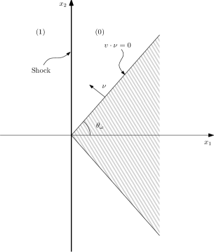
The analysis of 2-D steady supersonic flows past wedges whose vertex angles are less than the critical angle can date back to the 1940s since the stability of such flows is fundamental in applications (cf. [84, 205]). Local solutions around the wedge vertex were first constructed in Gu [119], Li [146], and Schaeffer [180]. Also see Zhang [212] and the references cited therein for global potential solutions when the wedges are a small perturbation of the straight-sided wedge. For the wedge problem, when the vertex angle is suitably large, the flow contains a large shock-front and, for this case, the full Euler equations (4.1) are required to describe the physical flow. When a wedge is straight and its vertex angle is less than the critical angle $\omega_{c}$, there exists a supersonic shock-front emanating from the wedge vertex so that the constant states on both sides of the shock are supersonic; the critical angle condition is necessary and sufficient for the existence of the supersonic shock (also see [69, 84]).

Consider 2-D steady supersonic Euler flows past a 2-D Lipschitz curved wedge $|x_{2}|\leq g(x_{1}),x_{1}>0$, with $g\in Lip({\mathbb{R}}_{+})$ and $g(0)=0$, whose vertex angle $\omega_{0}:=\arctan(g^{\prime}(0+))$ is less than the critical angle $\omega_{c}$, along which $TV\{g^{\prime}(\cdot);\,{\mathbb{R}}_{+}\}\leq\varepsilon$ for some constant $\varepsilon>0$. Denote

$$\Omega:=\{{\bf x}\,:\,x_{2}>g(x_{1}),\,x_{1}\geq 0\},\quad\Gamma:=\{{\bf x}\,:\,x_{2}=g(x_{1}),\,x_{1}\geq 0\},$$

and ${\bf n}(x_{1}\pm)=\frac{(-g^{\prime}(x_{1}\pm),1)}{\sqrt{(g^{\prime}(x_{1}\pm))^{2}+1}}$ are the outer normal vectors to $\Gamma$ at points $x_{1}\pm$, respectively. The uniform upstream flow ${\bf u}_{-}=(\rho_{-},\rho_{-}u_{-},0,\rho_{-}E_{-})$ satisfies $u_{-}>c(\rho_{-},S_{-})$ so that a strong supersonic shock-front emanates from the wedge vertex. Since the problem is symmetric with respect to the $x_{2}$-axis, the wedge problem can be formulated into the following problem of initial-boundary value type for system (4.1) in $\Omega$:

Cauchy Condition: $${\bf u}|_{x_{1}=0}={\bf u}_{-};\qquad\qquad\qquad$$ (4.2)

$$\mbox{\it Boundary Condition}:\qquad\qquad {\bf v}\cdot{\bf n}=0\qquad\mbox{ on }\,\Gamma.\qquad\qquad\qquad$$ (4.3)

In Chen-Zhang-Zhu [69], it has been established that there exist ${\varepsilon}_{0}>0$ and $C>0$ such that, when ${\varepsilon}\leq{\varepsilon}_{0}$, there exists a pair of functions

$${\bf u}=(\rho,{\bf v},\rho E)\in BV({\mathbb{R}};{\mathbb{R}}^{2}\times{\mathbb{R}}_{+}\times{\mathbb{R}}_{+}),\qquad\sigma\in BV({\mathbb{R}}_{+};{\mathbb{R}})$$

with $\chi=\int_{0}^{x_{1}}\sigma(s)ds\in Lip({\mathbb{R}}_{+};{\mathbb{R}}_{+})$ such that ${\bf u}$ is a global entropy solution of problem (4.1)–(4.3) in $\Omega$ with

$$TV\{{\bf u}(x_{1},\cdot)\,:\,[g(x_{1}),-\infty)\}\leq C\,TV\{g^{\prime}(\cdot)\}\quad\mbox{for every}\,\,\,x_{1}\in{\mathbb{R}}_{+},$$ (4.4)

and the strong shock-front $x_{2}=\chi(x_{1})$ emanating from the wedge vertex is nonlinearly stable in structure. Furthermore, the global $L^{1}$-stability of entropy solutions with respect to the incoming flow at $x_{1}=0$ in $L^{1}$ has also been established in Chen-Li [58]. This asserts that any supersonic shock-front for the wedge problem is nonlinearly $L^{1}$–stable with respect to the $BV$ perturbation of the incoming flow and the wedge boundary.

In order to achieve this, we have first developed an adaptation of the Glimm scheme whose mesh grids are designed to follow the slope of the Lipschitz wedge boundary so that the lateral Riemann building blocks contain only one shock or rarefaction wave emanating from the mesh points on the boundary. Such a design makes the $BV$ estimates more convenient for the Glimm approximate solutions. Then careful interaction estimates have been made. One of the essential estimates is the estimate of the strength $\delta_{1}$ of the reflected 1-waves in the interaction between the 4-strong shock-front and weak waves $(\alpha_{1},\beta_{2},\beta_{3},\beta_{4})$, that is,

$$\delta_{1}=\alpha_{1}+K_{s1}\beta_{4}+O(1)|\alpha_{1}|(|\beta_{2}|+|\beta_{3}|)\qquad\mbox{with}\,\,\,\,|K_{s1}|<1.$$

The second essential estimate is the interaction estimate between the wedge boundary and weak waves. Based on the construction of the approximation solutions and interaction estimates, we have successfully identified a Glimm-type functional to incorporate the curved wedge boundary and the strong shock-front naturally and to trace the interactions not only between the wedge boundary and weak waves, but also between the strong shock-front and weak waves. With the aid of the important fact that $|K_{s1}|<1$, we have showed that the identified Glimm functional monotonically decreases in the flow direction. Another essential estimate is to trace the approximate strong shock-fronts in order to establish the nonlinear stability and asymptotic behavior of the strong shock-front emanating from the wedge vertex under the $BV$ wedge perturbation.

For the 3-D cone problem, the nonlinear stability of a self-similar 3-D full gas flow past an infinite cone is another important problem. See Lien-Liu [140] for the cones with small vertex angle. Also see [71, 77] for the construction of piecewise smooth potential flows under smooth perturbation of the straight-sided cone.

In Elling-Liu [101], an evidence has been provided that the steady supersonic weak shock solution is dynamically stable, in the sense that it describes the long-time behavior of an unsteady flow.

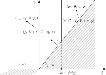
4.2. Stability of Supersonic Vortex Sheets

Another natural problem is the stability of supersonic vortex sheets above the Lipschitz wall $x_{2}=g(x_{1}),x_{1}\geq 0,$ with

$$g\in Lip({\mathbb{R}}_{+};{\mathbb{R}}),\,\,\,g(0)=g^{\prime}(0+)=0,\,\,\,\lim\limits_{x_{1}\to\infty}\arctan(g^{\prime}(x_{1}+))=0,$$

and $g^{\prime}\in BV({\mathbb{R}}_{+};{\mathbb{R}})$ such that $TV\{g^{\prime}(\cdot)\}\leq\varepsilon$ for some $\varepsilon>0$. Denote again $\Omega=\{{\bf x}\,:\,x_{2}>g(x_{1}),\,x_{1}\geq 0\}$ and $\Gamma=\{{\bf x}\,:\,x_{2}=g(x_{1}),\,x_{1}\geq 0\}$. The upstream flow consists of one supersonic straight vortex sheet $x_{2}=y_{0}>0$ and two constant vectors ${\bf u}_{0}=(\rho_{0},\rho_{0}u_{0},0,\rho_{0}E_{0})$ when $x_{2}>y_{0}>0$ and ${\bf u}_{1}=(\rho_{1},\rho_{1}u_{1},0,\rho_{1}E_{1})$ when $0<x_{2}<y_{0}$ satisfying $u_{1}>u_{0}>0$ and $u_{i}>c(\rho_{i},S_{i})$ for $i=0,1$. Then the vortex sheet problem can be formulated into the following problem of initial-boundary value type for system (4.1):

Cauchy Condition: $${\bf u}|_{x_{1}=0}=\left\{\begin{array}[]{ll}{\bf u}_{0},\quad 0<x_{2}<y_{0},\\ {\bf u}_{1},\quad x_{2}>y_{0};\end{array}\right.\qquad$$ (4.7)

$$\mbox{\it Slip Boundary Condition}:\qquad {\bf v}\cdot{\bf n}=0\qquad\mbox{ on }\,\Gamma.\qquad$$ (4.8)

It has been proved that steady supersonic vortex sheets, as time-asymptotics, are stable in structure globally, even under the $BV$ perturbation of the Lipschitz walls in Chen-Zhang-Zhu [70]. The result indicates that the strong supersonic vortex sheets are nonlinearly stable in structure globally under the $BV$ perturbation of the Lipschitz wall, although there may be weak shocks and supersonic vortex sheets away from the strong vortex sheet. In order to establish this theorem, as in §4.1, we first developed an adaption of the Glimm scheme whose mesh grids are designed to follow the slope of the Lipschitz boundary. For this case, one of the essential estimates is the estimate of the strength $\delta_{1}$ of the reflected 1-wave in the interaction between the 4-weak wave $\alpha_{4}$ and the strong vortex sheet from below is less than one: $\delta_{1}=K_{01}\alpha_{4}$ and $|K_{01}|<1$. The second new essential estimate is the estimate of the strength $\delta_{4}$ of the reflected 4-wave in the interaction between the 1-weak wave $\beta_{1}$ and the strong vortex sheet from above is also less than one: $\delta_{4}=K_{11}\beta_{1}$ and $|K_{11}|<1$. Another essential estimate is to trace the approximate supersonic vortex sheets under the $BV$ boundary perturbation. For more details, see Chen-Zhang-Zhu [70]. The nonlinear $L^{1}$-stability of entropy solutions with respect to the incoming flow at $x_{1}=0$ is under current investigation.

5. Multidimensional Steady Transonic Problems

In this section we discuss another important class of M-D steady problems: transonic problems. In the last decade, a program has been initiated on the existence and stability of M-D transonic shock-fronts, and some new analytical approaches including techniques, methods, and ideas have been developed. For clear presentation, we focus mainly on the celebrated steady potential flow equation of aerodynamics for the velocity potential $\varphi:\Omega\subset{{\mathbb{R}}}^{d}\rightarrow{{\mathbb{R}}}$, which is a second-order nonlinear PDE of mixed elliptic-hyperbolic type:

$$\nabla_{\bf x}\cdot(\rho(|\nabla_{\bf x}\varphi|^{2})\nabla_{\bf x}\varphi)=0,\qquad{\bf x}\in\Omega\subset{{\mathbb{R}}}^{d},$$ (5.1)

where the density $\rho(q^{2})$ by scaling is

$$\rho(q^{2})=\big{(}1-\frac{\gamma-1}{2}q^{2}\big{)}^{\frac{1}{\gamma-1}}$$ (5.2)

with adiabatic exponent $\gamma>1$. Equation (5.1) is elliptic at $\nabla_{\bf x}\varphi$ with $|\nabla_{\bf x}\varphi|=q$ if $\rho(q^{2})+2q^{2}\rho^{\prime}(q^{2})>0,$ which is equivalent to

$$q<q_{*}:=\sqrt{2/(\gamma+1)},$$

i.e., the flow is subsonic. Equation (5.1) is hyperbolic if $\rho(q^{2})+2q^{2}\rho^{\prime}(q^{2})<0,$ i.e., $q>q_{*}$, that is, the flow is supersonic.

Let $\Omega^{+}$ and $\Omega^{-}$ be open subsets of $\Omega$ such that $\Omega^{+}\cap\Omega^{-}=\emptyset$, $\overline{\Omega^{+}}\cup\overline{\Omega^{-}}=\overline{\Omega}$, and ${\mathcal{S}}=\partial\Omega^{+}\cap\Omega$. Let $\varphi\in C^{0,1}(\Omega)\cap C^{1}(\overline{\Omega^{\pm}})$ be a weak solution of (5.1), which satisfies $\displaystyle|\nabla_{\bf x}\varphi|\leq q_{cav}:=\sqrt{2/(\gamma-1)}$, so that $\nabla_{\bf x}\varphi$ experiences a jump across ${\mathcal{S}}$ that is a $(d-1)$-D smooth surface. Set $\varphi^{\pm}=\varphi|_{\Omega^{\pm}}$. Then $\varphi$ satisfies the following Rankine-Hugoniot conditions on ${\mathcal{S}}$:

$$\varphi^{+}=\varphi^{-},$$ (5.3)

$$\rho(|\nabla_{\bf x}\varphi^{+}|^{2})\nabla_{\bf x}\varphi^{+}\cdot{\bf n}=\rho(|\nabla_{\bf x}\varphi^{-}|^{2})\nabla_{\bf x}\varphi^{-}\cdot{\bf n}.$$ (5.4)

Suppose that $\varphi\in C^{1}(\overline{\Omega^{\pm}})$ is a weak solution satisfying

$$|\nabla_{\bf x}\varphi|<q_{*}\,\,\mbox{in }\,\Omega^{+},\;\;\quad|\nabla_{\bf x}\varphi|>q_{*}\,\,\mbox{in }\;\Omega^{-},\;\;\quad\nabla_{\bf x}\varphi^{\pm}\cdot{\bf n}|_{\mathcal{S}}>0.$$ (5.5)

Then $\varphi$ is a transonic shock-front solution with transonic shock-front ${\mathcal{S}}$ dividing $\Omega$ into the subsonic region $\Omega^{+}$ and the supersonic region $\Omega^{-}$ and satisfying the physical entropy condition (see Courant-Friedrichs [84]):

$$\rho(|\nabla_{\bf x}\varphi^{-}|^{2})<\rho(|\nabla_{\bf x}\varphi^{+}|^{2})\qquad\mbox{along}\,\,{\mathcal{S}}.$$ (5.6)

Note that equation (5.1) is elliptic in the subsonic region and hyperbolic in the supersonic region.

As an example, let $(x_{1},{\bf x}^{\prime})$ be the coordinates in ${{\mathbb{R}}}^{d}$, where $x_{1}\in{{\mathbb{R}}}$ and ${\bf x}^{\prime}=(x_{2},\dots,x_{d})\in{{\mathbb{R}}}^{d-1}$. Fix ${\bf V}_{0}\in{{\mathbb{R}}}^{d}$, and let $\varphi_{0}({\bf x}):={\bf V}_{0}\cdot{\bf x}$, ${\bf x}\in{{\mathbb{R}}}^{d}$. If $\displaystyle|{\bf V}_{0}|\in(0,q_{*})$ (resp. $\displaystyle|{\bf V}_{0}|\in(q_{*},q_{cav})$), then $\varphi_{0}({\bf x})$ is a subsonic (resp. supersonic) solution in ${{\mathbb{R}}}^{d}$, and ${\bf V}_{0}=\nabla_{\bf x}\varphi_{0}$ is its velocity.

Let $q^{-}_{0}>0$ and ${\bf V}^{\prime}_{0}\in{{\mathbb{R}}}^{d-1}$ be such that the vector ${\bf V}^{-}_{0}:=(q^{-}_{0},{\bf V}^{\prime}_{0})$ satisfies $|{\bf V}^{-}_{0}|>q_{*}$. Then there exists a unique $q^{+}_{0}>0$ such that

$$\big{(}1-\frac{\gamma-1}{2}(|q^{+}_{0}|^{2}+|{\bf V}^{\prime}_{0}|^{2})\big{)}^{\frac{1}{\gamma-1}}q^{+}_{0}=\big{(}1-\frac{\gamma-1}{2}(|q^{-}_{0}|^{2}+|{\bf V}^{\prime}_{0}|^{2})\big{)}^{\frac{1}{\gamma-1}}q^{-}_{0}.$$ (5.7)

The entropy condition (5.6) implies $q^{+}_{0}<q^{-}_{0}$. By denoting ${\bf V}^{+}_{0}:=(q^{+}_{0},{\bf V}^{\prime}_{0})$ and defining the functions $\varphi_{0}^{\pm}({\bf x}):=V^{\pm}_{0}\cdot{\bf x}$ on ${{\mathbb{R}}}^{d}$, then $\varphi_{0}^{+}$ (resp. $\varphi_{0}^{-}$) is a subsonic (resp. supersonic) solution. Furthermore, from (5.4) and (5.7), the function

$$\varphi_{0}({\bf x}):=\min(\varphi_{0}^{-}({\bf x}),\varphi_{0}^{+}({\bf x}))=V^{\pm}_{0}\cdot{\bf x},\,\,\,\,\,\,{\bf x}\in\Omega^{\pm}_{0}:=\{\pm x_{1}>0\},$$ (5.8)

is a plane transonic shock-front solution in ${{\mathbb{R}}}^{d}$, $\Omega^{-}_{0}$ and $\Omega^{+}_{0}$ are respectively its supersonic and subsonic regions, and ${\mathcal{S}}=\{x_{1}=0\}$ is a transonic shock-front. Note that, if ${\bf V}^{\prime}_{0}=0$, the velocities $V^{\pm}_{0}$ are orthogonal to the shock-front ${\mathcal{S}}$ and, if ${\bf V}^{\prime}_{0}\neq 0$, the velocities are not orthogonal to ${\mathcal{S}}$.

5.1. Transonic Shock-Front Problems in ${\mathbb{R}}^{d}$

Consider M-D perturbations of the uniform transonic shock-front solution (5.8) in ${{\mathbb{R}}}^{d}$ with $d\geq 3$. Since it suffices to specify the supersonic perturbation $\varphi^{-}$ only in a neighborhood of the unperturbed shock-front $\{x_{1}=0\}$, we introduce domains $\Omega:=(-1,\infty)\times{{\mathbb{R}}}^{d-1},\Omega_{1}:=(-1,1)\times{{\mathbb{R}}}^{d-1}.$ Note that we expect the subsonic region $\Omega^{+}$ to be close to the half-space $\Omega^{+}_{0}=\{x_{1}>0\}$.

Problem 5.1. Given a supersonic solution $\varphi^{-}({\bf x})$ of (5.1) in $\Omega_{1}$, find a transonic shock-front solution $\varphi({\bf x})$ in $\Omega$ such that

$$\Omega^{-}\subset\Omega_{1},\qquad\varphi({\bf x})=\varphi^{-}({\bf x})\,\,\,\,\,\mbox{ in}\,\,\Omega^{-},$$

where $\Omega^{-}:=\Omega\setminus\Omega^{+}$ and $\Omega^{+}:=\{{\bf x}\in\Omega\;:\;|\nabla_{\bf x}\varphi({\bf x})|<q_{*}\}$, and

$$\varphi=\varphi^{-},\quad\partial_{x_{1}}\varphi=\partial_{x_{1}}\varphi^{-}\qquad\mbox{on }\{x_{1}=-1\},$$ (5.9)

$$\lim_{R\to\infty}\|\varphi-\varphi^{+}_{0}\|_{C^{1}(\Omega^{+}\setminus B_{R}(0))}=0.$$ (5.10)

Condition (5.9) determines that the solution has supersonic upstream, while condition (5.10) especially determines that the uniform velocity state at infinity in the downstream direction is equal to the unperturbed downstream velocity state. The additional requirement in (5.10) that $\varphi\to\varphi^{+}_{0}$ at infinity within $\Omega^{+}$ fixes the position of shock-front at infinity. This allows us to determine the solution of Problem 5.1 uniquely. In Chen-Feldman [47], we have employed the free boundary approach first developed for the potential flow equation (5.1) to solve the stability problem, Problem 5.1. This existence result can be extended to the case that the regularity of the steady perturbation $\varphi^{-}$ is only $C^{1,1}$. It would be interesting to establish similar results for the full Euler equations (1.4).

5.2. Nozzle Problems Involving Transonic Shock-Fronts

We now consider M-D transonic shock-fronts in the following infinite nozzle ${\Omega}$ with arbitrary smooth cross-sections: ${\Omega}={\Psi}({\Lambda}\times{\mathbb{R}})\cap\{x_{1}>-1\}$, where ${\Lambda}\subset{{\mathbb{R}}}^{d-1}$ is an open bounded connected set with a smooth boundary, and ${\Psi}:{{\mathbb{R}}}^{d}\to{{\mathbb{R}}}^{d}$ is a smooth map, which is close to the identity map. For simplicity, we assume that $\partial{\Lambda}$ is in $\displaystyle C^{[\frac{d}{2}]+3,\alpha}$ and $\|{\Psi}-I\|_{[\frac{d}{2}]+3,\alpha,{{\mathbb{R}}}^{d}}\leq\sigma$ for some $\alpha\in(0,1)$ and small $\sigma>0$, where $[s]$ is the integer part of $s$, $I:{{\mathbb{R}}}^{d}\to{{\mathbb{R}}}^{d}$ is the identity map, and $\partial_{l}{\Omega}:={\Psi}({\mathbb{R}}\times\partial{\Lambda})\cap\{x_{1}>-1\}$. For concreteness, we also assume that there exists $L>1$ such that ${\Psi}({\bf x})={\bf x}$ for any ${\bf x}=(x_{1},{\bf x}^{\prime})$ with $x_{1}>L$.

In the 2-D case, ${\Omega}=\{(x_{1},x_{2})\;:\;x_{1}>-1,\;b^{-}(x_{2})<x_{2}<b^{+}(x_{2})\},$ where $\|b^{\pm}-b^{\pm}_{\infty}\|_{4,\alpha,{{\mathbb{R}}}}\leq\sigma$ and $b^{\pm}\equiv b^{\pm}_{\infty}$ on $[L,\infty)$ for some constants $b^{\pm}_{\infty}$ satisfying $b^{+}_{\infty}>b^{-}_{\infty}$. For the M-D case, the geometry of the nozzles is much richer. Note that our setup implies that $\partial{\Omega}=\overline{\partial_{o}{\Omega}}\cup\partial_{l}{\Omega}$ with

$$\partial_{l}{\Omega}:={\Psi}[(-\infty,\infty)\times\partial{\Lambda}]\cap\{(x_{1},{\bf x}^{\prime})\;:\;x_{1}>-1\},$$

$$\partial_{o}{\Omega}:={\Psi}((-\infty,\infty)\times{\Lambda})\cap\{(x_{1},{\bf x}^{\prime})\;:\;x_{1}=-1\}.$$

Then our transonic nozzle problem can be formulated as

Problem 5.2: Transonic Nozzle Problem. Given the supersonic upstream flow at the entrance $\partial_{o}\Omega$:

$$\varphi=\varphi^{-}_{e},\,\,\,\,\varphi_{x_{1}}=\psi^{-}_{e}\qquad\mbox{on }\partial_{o}{\Omega},$$ (5.11)

the slip boundary condition on the nozzle boundary $\partial_{l}{\Omega}$:

$$\nabla_{\bf x}\varphi\cdot{\bf n}=0\qquad\mbox{on }\mbox{$\partial_{l}{\Omega}$},$$ (5.12)

and the uniform subsonic flow condition at the infinite exit $x_{1}=\infty$:

$$\|\varphi(\cdot)-q_{\infty}x_{1}\|_{C^{1}({\Omega}\cap\{x_{1}>R\})}\to 0\qquad\,\mbox{as }R\to\infty\,\,\mbox{for some }q_{\infty}\in(0,q_{*}),$$ (5.13)

find a M-D transonic flow $\varphi$ of problem (5.1) and (5.11)–(5.13) in $\Omega$.

The standard local existence theory of smooth solutions for the initial-boundary value problem (5.11)–(5.12) for second-order quasilinear hyperbolic equations implies that, as $\sigma$ is sufficiently small, there exists a supersonic solution $\varphi^{-}$ of (5.1) in $\Omega_{2}:=\{-1\leq x_{1}\leq 1\},$ which is a $C^{l+1}$ perturbation of $\varphi_{0}^{-}=q_{0}^{-}x_{1}$: For any $\alpha\in(0,1]$,

$$\|\varphi^{-}-\varphi_{0}^{-}\|_{l,\alpha,{\Omega}_{2}}\leq C_{0}\sigma,\qquad l=1,2,$$ (5.14)

for some constant $C_{0}>0$, and satisfies $\nabla\varphi^{-}\cdot{\bf n}=0$ on $\partial_{l}{\Omega}_{2}$, provided that $(\varphi^{-}_{e},\psi^{-}_{e})$ on $\partial_{o}\Omega$ satisfying

$$\|\varphi_{e}^{-}-q_{0}^{-}x_{1}\|_{H^{s+l}}+\|\psi_{e}^{-}-q_{0}^{-}\|_{H^{s+l-1}}\leq\sigma,\qquad l=1,2,$$ (5.15)

for some integer $s>{d}/{2}+1$ and the compatibility conditions up to order $s+1$, where the norm $\|\cdot\|_{H^{s}}$ is the Sobolev norm with $H^{s}=W^{s,2}$.

In Chen-Feldman [48], Problem 5.2 has been solved. More precisely, let $\displaystyle q^{-}_{0}\in(q_{*},q_{cav})$ and $\displaystyle q^{+}_{0}\in(0,q_{*})$ satisfy (5.7), and let $\varphi_{0}$ be the transonic shock-front solution (5.8) with ${\bf V}^{\prime}=0$. Then there exist $\sigma_{0}>0$ and $C$, depending only on $d$, $\alpha$, $\gamma$, $q^{-}_{0}$, ${\Lambda}$, and $L$, such that, for every $\sigma\in(0,\sigma_{0})$, any map ${\Psi}$ introduced above, and any supersonic upstream flow $(\varphi^{-}_{e},\psi^{-}_{e})$ on $\partial_{o}\Omega$ satisfying (5.15) with $l=1$, there exists a solution $\varphi\in C^{0,1}({\Omega})\cap C^{1,\alpha}(\overline{\Omega^{+}})$ satisfying

$$\Omega^{+}(\varphi)=\{x_{1}>f({\bf x}^{\prime})\},\qquad\Omega^{-}(\varphi)=\{x_{1}<f({\bf x}^{\prime})\},$$

$$\|\varphi-q^{\pm}x_{1}\|_{1,\alpha,\Omega^{\pm}}\leq C\sigma,\qquad\|\varphi-q_{\infty}x_{1}\|_{C^{1}({\Omega}\cap\{x_{1}>R\})}\to 0\,\,\mbox{as $R\to\infty$},$$

where $q_{\infty}\in(0,q_{*})$ is the unique solution of the equation

$$\rho((q^{+})^{2})q^{+}=Q^{+}:=\frac{1}{|{\Lambda}|}\int_{\partial_{o}{\Omega}}\rho(|\nabla_{{\bf x}^{\prime}}\varphi_{e}^{-}|^{2}+(\psi_{e}^{-})^{2})\psi_{e}^{-}\,d{{\mathcal{H}}^{d-1}}.$$ (5.16)

In addition, if the supersonic uniform flow $(\varphi_{e}^{-},\psi_{e}^{-})$ on $\partial_{o}\Omega$ satisfies (5.15) with $l=2$, then $\varphi\in C^{2,\alpha}(\overline{\Omega^{+}})$ with $\|\varphi-q^{+}x_{1}\|_{2,\alpha,\Omega_{+}}\leq C\sigma,$ and the solution with a transonic shock-front is unique and stable with respect to the nozzle boundary and the smooth supersonic upstream flow at the entrance. The techniques have been extended to solving the nozzle problem for the 2-D full Euler equations first in Chen-Chen-Feldman [43].

In the previous setting, the location of the transonic shock-front in the solution is not unique in general if we prescribe only the pressure at the nozzle exit, since the flat shock-front between uniform states can be translated along the flat nozzle which does not change the flow parameters at the entrance and the pressure at the exit. The analysis of the relation among the unique shock-front location, the flow parameters, and the geometry of the diverging nozzle has been made for various Euler systems in different dimensions; see Chen [73] and Lin-Yuan [153] for the 2-D full Euler equations, Li-Xin-Yin [145] for the 2-D and 3-D axisymmetric Euler systems with narrow divergent nozzles, and Bae-Feldman [9] for perturbed diverging cone-shaped nozzle of arbitrary cross-section for the non-isentropic potential flow system in any dimension.

A major open problem is the physical de Laval nozzle problem: Consider a nozzle $\Omega$ which is flat (i.e., $\Psi=I$) between $-2\leq x_{1}\leq-1$ and $1\leq x_{1}\leq\infty$, and has some special geometry between $-1\leq x_{1}\leq 1$ to make the part $\{-1\leq x_{1}\leq 0\}$ convergent and the part $\{0\leq x_{1}\leq 1\}$ divergent. Given certain incoming subsonic flow at $x_{1}=-2$, find a transonic flow containing transonic shock-fronts in the nozzle such that the downstream at $x_{1}=\infty$ is subsonic. A related reference is Kuz’min’s book [135].

5.3. Wedge/Cone Problems Involving Transonic Shock-Fronts

The existence and stability of transonic flows past infinite wedges or cones are further long-standing open transonic problems. Some progress has been made for the wedge case in 2-D steady flow in Chen-Fang [75], Fang [104], and Chen-Chen-Feldman [44]. In [104], it was proved that the transonic shock-front is conditionally stable under perturbation of the upstream flow and/or the wedge boundary in some weak Sobolev norms. In [44], the existence and stability of transonic flows past the curved wedge have been established in the strong Hölder norms for the full Euler equations.

Conical flow (i.e. cylindrically symmetric flow with respect to an axis, say, the $x_{1}$-axis) in ${\mathbb{R}}^{3}$ occurs in many physical situations (cf. [84]). Unlike the 2-D case, the governing equations for the 3-D conical case have a singularity at the cone vertex and the flow past the straight-sided cone is self-similar, but is no longer piecewise constant. These have resulted in additional difficulties for the stability problem. In Chen-Fang [46], we have developed techniques to handle the singular terms in the equations and the singularity of the solutions. Our main results indicate that the self-similar transonic shock-front is conditionally stable with respect to the conical perturbation of the cone boundary and the upstream flow in appropriate function spaces. That is, the transonic shock-front and downstream flow in our solutions are close to the unperturbed self-similar transonic shock-front and downstream flow under the conical perturbation, and the slope of the shock-front asymptotically tends to the slope of the unperturbed self-similar shock-front at infinity.

In order to achieve these results, we have first formulated the stability problem as a free boundary problem and have then introduced a coordinate transformation to reduce the free boundary problem into a fixed boundary value problem for a singular nonlinear elliptic system. We have developed an iteration scheme that consists of two iteration mappings: one is for an iteration of approximate transonic shock-fronts; and the other is for an iteration of the corresponding boundary value problems for the singular nonlinear systems for given approximate shock-fronts. To ensure the well-definedness and contraction property of the iteration mappings, it is essential to establish the well-posedness for a corresponding singular linearized elliptic equation, especially the stability with respect to the coefficients of the equation, and to obtain the estimates of its solutions reflecting their singularity at the cone vertex and decay at infinity. The approach is to employ key features of the equation, introduce appropriate solution spaces, and apply a Fredholm-type theorem in Maz’ya-Plamenevskivı [161] to establish the existence of solutions by showing the uniqueness in the solution spaces. Also see Cui-Yin [87] for related results.

5.4. Airfoil/Obstacle Problems: Subsonic Flows past an Airfoil or an Obstacle

The Euler equations for potential flows (5.1)–(5.2) in ${\mathbb{R}}^{2}$ can be rewritten as

$$\begin{cases}\partial_{x_{1}}v-\partial_{x_{2}}u=0,\\ \partial_{x_{1}}(\rho u)+\partial_{x_{2}}(\rho v)=0,\end{cases}$$ (5.17)

with $(u,v)=\nabla_{\bf x}\varphi$ and $q=|\nabla_{\bf x}\varphi|$, where $\rho$ is again determined by the Bernoulli relation (5.1). An important problem is subsonic flows past an airfoil or an obstacle. Shiffman [189], Bers [15], Finn-Gilbarg [106], and Dong [98] studied subsonic (elliptic) solutions of (5.1) outside an obstacle when the upstream flows are sufficiently subsonic; also see Chen-Dafermos-Slemrod-Wang [45] via compensated compactness argument. Morawetz in [166] first showed that the flows of (5.17) past an obstacle may contain transonic shocks in general. A further problem is to construct global entropy solutions of the airfoil problem (see [163, 110]).

In Chen-Slemrod-Wang [61], we have introduced the usual flow angle $\theta=\tan^{-1}(\frac{v}{u})$ and written the irrotationality and mass conservation equation as an artificially viscous problem:

$$\begin{cases}\partial_{x_{1}}v^{\varepsilon}-\partial_{x_{2}}u^{\varepsilon}=\varepsilon\Delta\theta^{\varepsilon},\\ \partial_{x_{1}}(\rho^{\varepsilon}u^{\varepsilon})+\partial_{x_{2}}(\rho^{\varepsilon}v^{\varepsilon})=\varepsilon\nabla\cdot(\sigma(\rho^{\varepsilon})\nabla\rho^{\varepsilon}),\end{cases}$$ (5.18)

where $\sigma(\rho)$ is suitably chosen, and appropriate boundary conditions are imposed for this regularized “viscous” problem. The crucial new discovery is that a uniformly $L^{\infty}$ bound in $q^{\varepsilon}$ can be obtained when $1\leq\gamma<3$ which uniformly prevents cavitation. However, in this formulation, a uniform bound in the flow angle $\theta^{\varepsilon}$ and a uniform lower bound in $q^{\varepsilon}$ in any fixed region disjoint from the profile must be assumed apriori. By making further careful energy estimates, Morawetz’s argument [163] then applies, and the strong convergence in $L^{1}_{\rm loc}(\Omega)$ of our approximating sequence is achieved.

An important open problem is whether two remaining conditions on $(q^{\varepsilon},\theta^{\varepsilon})$ can be removed. See Chen-Slemrod-Wang [61] for more details.

5.5. Nonlinear Approaches

We now discuss several nonlinear approaches to deal with steady transonic problems.

5.5.1. Free Boundary Approaches

We first describe two of the free boundary approaches for Problems 5.1–5.2, developed in [47, 48].

Free Boundary Problems. The transonic shock-front problems can be formulated into a one-phase free boundary problem for a nonlinear elliptic PDE: Given $\varphi^{-}\in C^{1,\alpha}(\overline{\Omega})$, find a function $\varphi$ that is continuous in $\Omega$ and satisfies

$$\varphi\leq\varphi^{-}\qquad\hbox{in}\,\,\bar{\Omega},$$ (5.19)

equation (5.1), the ellipticity condition in the non-coincidence set $\Omega^{+}=\{\varphi<\varphi^{-}\}$, the free boundary condition (5.4) on the boundary $\mathcal{S}=\partial\Omega^{+}\cap\Omega$, as well as the prescribed conditions on the fixed boundary $\partial\Omega$ and at infinity. These conditions are different in different problems, for example, conditions (5.9)–(5.10) for Problem 5.1 and (5.11)–(5.13) for Problem 5.2.

The free boundary is the location of the shock-front, and the free boundary conditions (5.3)–(5.4) are the Rankine-Hugoniot conditions. Note that condition (5.19) is motivated by the similar property (5.8) of unperturbed shock-fronts; and (5.19), locally on the shock-front, is equivalent to the entropy condition (5.6). Condition (5.19) transforms the transonic shock-front problem, in which the subsonic region $\Omega^{+}$ is determined by the gradient condition $|\nabla_{\bf x}\varphi({\bf x})|<q_{*}$, into a free boundary problem in which $\Omega^{+}$ is the non-coincidence set. In order to solve this free boundary problem, equation (5.1) is modified to be uniformly elliptic and then the free boundary condition (5.4) is correspondingly modified. The problem becomes a one-phase free boundary problem for the uniformly elliptic equation which we can solve. Since $\varphi^{-}$ is a small $C^{1,\alpha}$–perturbation of $\varphi^{-}_{0}$, the solution $\varphi$ of the free boundary problem is shown to be a small $C^{1,\alpha}$–perturbation of the given subsonic shock-front solution $\varphi^{+}_{0}$ in $\Omega^{+}$. In particular, the gradient estimate implies that $\varphi$ in fact satisfies the original free boundary problem, hence the transonic shock-front problem, Problem 5.1 (Problem 5.2, respectively).

The modified free boundary problem does not directly fit into the variational framework of Alt-Caffarelli [2] and Alt-Caffarelli-Friedman [3], and the regularization framework of Berestycki-Caffarelli-Nirenberg [17]. Also, the nonlinearity of the free boundary problem makes it difficult to apply the Harnack inequality approach of Caffarelli [30]. In particular, a boundary comparison principle for positive solutions of nonlinear elliptic equations in Lipschitz domains is not available yet for the equations that are not homogeneous with respect to $(\nabla^{2}_{\bf x}u,\nabla_{\bf x}u,u)$, which is our case.

Iteration Approach. The first approach we developed in Chen-Feldman [47, 48] for the steady potential flow equation is an iteration scheme based on the non-degeneracy of the free boundary condition: the jump of the normal derivative of a solution across the free boundary has a strictly positive lower bound. Our iteration process is as follows. Suppose that the domain $\Omega^{+}_{k}$ is given so that $S_{k}:=\partial\Omega^{+}_{k}\setminus\partial\Omega$ is $C^{1,\alpha}$. Consider the oblique derivative problem in $\Omega^{+}_{k}$ obtained by rewriting the (modified) equation (5.1) and free boundary condition (5.4) in terms of the function $u:=\varphi-\varphi^{+}_{0}$. Then the problem has the following form:

$$\begin{array}[]{ll}\displaystyle\mbox{div\,}_{\bf x}{\bf A}({\bf x},\nabla_{\bf x}u)=F({\bf x})&\mbox{ in }\;\Omega^{+}_{k}:=\{u>0\},\\ \displaystyle{\bf A}({\bf x},\nabla_{\bf x}u)\cdot{\bf n}=G({\bf x},{\bf n})&\mbox{ on }\;{\mathcal{S}}:=\partial\Omega^{+}_{k}\setminus\partial\Omega,\end{array}$$ (5.20)

plus the fixed boundary conditions on $\partial\Omega^{+}_{k}\cap\partial\Omega$ and the conditions at infinity. The equation is quasilinear, uniformly elliptic, ${\bf A}({\bf x},0)\equiv 0$, while $G({\bf x},{\bf n})$ has a certain structure. Let $u_{k}\in C^{1,\alpha}(\overline{\Omega_{k}^{+}})$ be the solution of (5.20). Then $\|u_{k}\|_{1,\alpha,\Omega^{+}_{k}}$ is estimated to be small if the perturbation is small, where appropriate weighted Hölder norms are actually needed in the unbounded domains. The function $\varphi_{k}:=\varphi^{+}_{0}+u_{k}$ from $\Omega^{+}_{k}$ is extended to $\Omega$ so that the $C^{1,\alpha}$–norm of $\varphi_{k}-\varphi^{+}_{0}$ in $\Omega$ is controlled by $\|u_{k}\|_{1,\alpha,\Omega_{k}^{+}}$. For the next step, define $\Omega^{+}_{k+1}:=\{{\bf x}\in\Omega\,:\,\varphi_{k}({\bf x})<\varphi^{-}({\bf x})\}.$ Note that, since $\|\varphi_{k}-\varphi^{+}_{0}\|_{1,\alpha,\Omega}$ and $\|\varphi^{-}-\varphi^{-}_{0}\|_{1,\alpha,\Omega}$ are small, we have $|\nabla_{\bf x}\varphi^{-}|-|\nabla_{\bf x}\varphi_{k}|\geq\delta>0$ in $\Omega$, and this nondegeneracy implies that $S_{k+1}:=\partial\Omega^{+}_{k+1}\setminus\partial\Omega$ is $C^{1,\alpha}$ and its norm is estimated in terms of the data of the problem.

The fixed point $\Omega^{+}$ of this process determines a solution of the free boundary problem since the corresponding solution $\varphi$ satisfies $\Omega^{+}=\{\varphi<\varphi^{-}\}$ and the Rankine-Hugoniot condition (5.4) holds on ${\mathcal{S}}:=\partial\Omega^{+}\cap\Omega$. On the other hand, the elliptic estimates alone are not sufficient to get the existence of a fixed point, because the right-hand side of the boundary condition in problem (5.20) depends on the unit normal ${\bf n}$ of the free boundary. One way is to require the orthogonality of the flat shock-fronts so that $\rho(|\nabla_{\bf x}\varphi_{0}^{+}|^{2})\nabla_{\bf x}\varphi_{0}^{+}=\rho(|\nabla_{\bf x}\varphi_{0}^{-}|^{2})\nabla_{\bf x}\varphi_{0}^{-}$ in $\Omega$ to obtain better estimates for the iteration and prove the existence of a fixed point. For more details, see Chen-Feldman [47, 48].

Partial Hodograph Approach. The second approach we have developed in [47] is a partial hodograph procedure, with which we can handle the existence and stability of M-D transonic shock-fronts that are not nearly orthogonal to the flow direction. One of the main ingredients in this new approach is to employ a partial hodograph transform to reduce the free boundary problem to a conormal boundary value problem for the corresponding nonlinear second-order elliptic equation of divergence form and then to develop techniques to solve the conormal boundary value problem. To achieve this, the strategy is to construct first solutions in the intersection domains between the physical unbounded domain under consideration and a series of half balls with radius $R$, then make uniform estimates in $R$, and finally send $R\to\infty$. It requires delicate apriori estimates to achieve this. A uniform bound in a weighted $L^{\infty}$-norm can be achieved by both employing a comparison principle and identifying a global function with the same decay rate as the fundamental solution of the elliptic equation with constant coefficients which controls the solutions. Then, by scaling arguments, the uniform estimates can be obtained in a weighted Hölder norm for the solutions, which lead to the existence of a solution in the unbounded domain with some decay rate at infinity. For such decaying solutions, a comparison principle holds, which implies the uniqueness for the conormal problem. Finally, by the gradient estimate, the limit function can be shown to be a solution of the M-D transonic shock problem, and then the existence result can be extended to the case that the regularity of the steady perturbation is only $C^{1,1}$. We can further prove that the M-D transonic shock-front solution is stable with respect to the $C^{2,\alpha}$ supersonic perturbation.

When the regularity of the steady perturbation is $C^{3,\alpha}$ or higher: $\|\varphi^{-}-\varphi_{0}^{-}\|^{(d-1)}_{3,\alpha,\Omega_{1}}\leq\sigma,$ we have introduced another simpler approach, the implicit function approach, to deal with the existence and stability problem in Chen-Feldman [47].

Other approaches can be found in Canic-Keyfitz-Lieberman [31], Canic-Keyfitz-Kim [33], Chen-Chen-Feldman [43], Chen [72, 73], Zheng [215], and the references cited therein.

5.5.2. Weak Convergence Approaches

Recent investigations on conservation laws based on weak convergence methods suggested that the method of compensated compactness be amenable to flows which exhibit both elliptic and hyperbolic regimes. In [163] (also see [164]), Morawetz layed out a program for proving the existence of the steady transonic flow problem about a bump profile in the upper half plane (which is equivalent to a symmetric profile in the whole plane). It was shown that, if the key hypotheses of the method of compensated compactness could be satisfied, now known as a “compactness framework” (see Chen [39]), then indeed there would exist a weak solution to the problem of flow over a bump which is exhibited by subsonic and supersonic regimes, i.e., transonic flow.

The compactness framework for system (5.17) can be formulated as follows. Let a sequence of functions ${\bf w}^{\varepsilon}({\bf x})=(u^{\varepsilon},v^{\varepsilon})({\bf x})$ defined on an open set $\Omega\subset{\mathbb{R}}^{2}$ satisfy the following set of conditions:

(A.1)  $q^{\varepsilon}({\bf x})=|{\bf w}^{\varepsilon}({\bf x})|\leq q_{\sharp}\;\;\hbox{a.e. in}\;\;\Omega$ for some positive constant $q_{\sharp}<q_{cav}$;

(A.2)   $\nabla_{\bf x}\cdot{\bf Q}_{\pm}({\bf w}^{\varepsilon})$   are confined in a compact set in $H^{-1}_{\rm loc}(\Omega)$ for entropy pairs ${\bf Q}_{\pm}=(Q_{1\pm},Q_{2\pm})$, where ${\bf Q}_{\pm}({\bf w}^{\varepsilon})$ are confined to a bounded set uniformly in $L_{\rm loc}^{\infty}(\Omega)$.

When (A.1) and (A.2) hold, the Young measure $\nu_{{\bf x}}({\bf w}),{\bf w}=(u,v)$, determined by the uniformly bounded sequence of functions ${\bf w}^{\varepsilon}$ is constrained by the following commutator relation:

$$\langle\nu_{\bf x},\;Q_{1+}Q_{2-}-Q_{1-}Q_{2+}\rangle=\langle\nu_{\bf x},\;Q_{1+}\rangle\langle\nu_{\bf x},\;Q_{2-}\rangle-\langle\nu_{\bf x},\;Q_{1-}\rangle\langle\nu_{\bf x},\;Q_{2+}\rangle.$$ (5.21)

The main point for the compensated compactness framework is to prove that $\nu_{{\bf x}}$ is a Dirac mass by using entropy pairs, which implies the compactness of the sequence ${\bf w}^{\varepsilon}({\bf x})=(u^{\varepsilon},v^{\varepsilon})({\bf x})$ in $L^{1}_{\rm loc}(\Omega)$. In this context, It is needed Morawetz [163] to presume the existence of an approximating sequence parameterized by $\varepsilon$ to their problems satisfying (A.1) and (A.2) so that they could exploit the commutator identity and obtain the strong convergence in $L^{1}_{\rm loc}(\Omega)$ to a weak solution of their problems.

As it turns out, there is a classical problem where (A.1) and (A.2) hold trivially, i.e., the sonic limit of subsonic flows. In that case, we return to the result by Bers [15] and Shiffman [189], which says that, if the speed at infinity, $q_{\infty}$, is less than some $\hat{q}$, there is a smooth unique solution of the problem and ask what happens as $q_{\infty}\nearrow\hat{q}$. In this case, the flow develops sonic points and the governing equations become degenerate elliptic. Thus, if we set $\varepsilon=\hat{q}-q_{\infty}$ and examine a sequence of exact smooth solutions to our system, we see trivially that (A.1) is satisfied since $|q^{\varepsilon}|\leq q_{*}$, and (A.2) is also satisfied since $\nabla_{\bf x}\cdot{\bf Q}_{\pm}({\bf w}^{\varepsilon})=0$ along our solution sequence. The effort is in finding entropy pairs which guarantee the Young measure $\nu_{{\bf x}}$ reduces to a Dirac mass. Ironically, the original conservation equations of momentum in fact provide two sets of entropy pairs, while the irrotationality and mass conservation equations provide another two sets. This observation has been explored in detail in Chen-Dafermos-Slemrod-Wang [45].

What then about the fully transonic problem of flow past an obstacle or bump where $q_{\infty}>\hat{q}$? In Chen-Slemrod-Wang [61], we have provided some of the ingredients to satisfying (A.1) and (A.2) as explained in §5.4. On the other hand, (A.2) is easily obtained from the viscous formulation by using a special entropy pair of Osher-Hafez-Whitlow [172]. In fact, this entropy pair is very important: It guarantees that the inviscid limit of the above viscous system satisfies a physically meaningful “entropy” condition (Theorem 2 of [172]). With (A.1) and (A.2) satisfied, the compensated compactness argument then applies, to yield the strong convergence in $L^{1}_{\rm loc}(\Omega)$ of our approximate solutions.

Some further compensated compactness frameworks have been developed for solving the weak continuity of solutions to the Gauss-Codazzi-Ricci equations in Chen-Slemrod-Wang [62, 63]. Also see Dacorogna [88], Evans [103], and the references cited therein for various weak convergence methods and techniques.

6. Shock Reflection-Diffraction and Self-Similar Solutions

One of the most challenging problems is to study solutions with data that give rise to self-similar solutions (such solutions include Riemann solutions). For the Euler equations (1.4) for ${\bf x}\in{\mathbb{R}}^{2}$, the self-similar solutions

$$(\rho,{\bf v},p)=(\rho,{\bf v},p)(\xi,\eta),\qquad(\xi,\eta)={\bf x}/{t},$$ (6.1)

are determined by

$$\left\{\begin{array}[]{l}\partial_{\xi}(\rho U)+\partial_{\eta}(\rho V)=-2\rho,\\ \partial_{\xi}(\rho U^{2}+p)+\partial_{\eta}(\rho UV)=-3\rho U,\\ \partial_{\xi}(\rho UV)+\partial_{\eta}(\rho V^{2}+p)=-3\rho V,\\ \partial_{\xi}(\rho U(E+p/\rho))+\partial_{\eta}(\rho V(E+p/\rho))=-2\rho(E+p/\rho),\end{array}\right.$$ (6.2)

where $(U,V)={\bf v}-(\xi,\eta)$ is the pseudo-velocity and $E=e+\frac{1}{2}(U^{2}+V^{2})$.

The four eigenvalues are

$$\lambda_{0}=\frac{V}{U}\,\,\,\mbox{(2-multiplicity)},\qquad\lambda_{\pm}=\frac{UV\pm c\sqrt{U^{2}+V^{2}-c^{2}}}{U^{2}-c^{2}},$$

where $c=\sqrt{p_{\rho}(\rho,S)}$ is the sonic speed. When $U^{2}+V^{2}>c^{2}$, system (6.2) is hyperbolic with four real eigenvalues and the flow is called pseudo-supersonic, simply called supersonic without confusion. When $U^{2}+V^{2}<c^{2}$, system (6.2) is hyperbolic-elliptic composite type (two repeated eigenvalues are real and the other two are complex): two equations are hyperbolic and the other two are elliptic. The region $U^{2}+V^{2}=c^{2}$ in the $(\xi,\eta)$-plane is simply called the sonic region in the flow. In general, system (6.2) is hyperbolic-elliptic mixed and composite type, and the flow is transonic. For a bounded solution $(\rho,{\bf v},p)$, the flow must be supersonic when $\xi^{2}+\eta^{2}\to\infty$.

An important prototype problem for both practical applications and the theory of M-D complex wave patterns is the problem of diffraction of a shock-front which is incident along an inclined ramp. When a plane shock-front hits a wedge head on, a self-similar reflected shock-front moves outward as the original shock-front moves forward (cf. [13, 34, 84, 116, 165, 183, 201]). Then the problem of shock reflection-diffraction by a wedge can be formulated as follows:

Problem 6.1 (Initial-boundary value problem). Seek a solution of system (1.4) satisfying the initial condition at $t=0$:

$$(\rho,{\bf v},p)=\begin{cases}(\rho_{0},0,0,p_{0}),&\,\quad|x_{2}|>x_{1}\tan\theta_{w},x_{1}>0,\\ (\rho_{0},u_{1},0,p_{1}),&\,\quad x_{1}<0;\end{cases}$$ (6.3)

and the slip boundary condition along the wedge boundary:

$${\bf v}\cdot{\bf n}=0,$$ (6.4)

where ${\bf n}$ is the exterior unit normal to the wedge boundary, and state $(0)$ and $(1)$ satisfy

$$u_{1}=\sqrt{\frac{(p_{1}-p_{0})(\rho_{1}-\rho_{0})}{\rho_{0}\rho_{1}}},\,\,\frac{p_{1}}{p_{0}}=\frac{(\gamma+1)\rho_{1}-(\gamma-1)\rho_{0}}{(\gamma+1)\rho_{0}-(\gamma-1)\rho_{1}},\,\,\,\rho_{1}>\rho_{0}.$$ (6.5)

Given $\rho_{0},p_{0},\rho_{1}$, and $\gamma>1$, the other variables $u_{1}$ and $p_{1}$ are determined by (6.5). In particular, the Mach number $M_{1}=\frac{u_{1}}{c_{1}}$ for state (1) is determined by $M_{1}^{2}=\frac{2(\rho_{1}-\rho_{0})^{2}}{\rho_{0}((\gamma+1)\rho_{1}-(\gamma-1)\rho_{0})}$.

Figure 1. Initial-boundary value problem

Since the initial-boundary value problem, Problem 6.1, is invariant under the self-similar scaling, we seek self-similar solutions (6.1) governed by system (6.2). Since the problem is symmetric with respect to the axis $\eta=0$, it suffices to consider the problem in the half-plane $\eta>0$ outside the half-wedge:

$$\Lambda:=\{\xi<0,\eta>0\}\cup\{\eta>\xi\tan\theta_{w},\,\xi>0\}.$$

Then Problem 6.1 in the $(t,{\bf x})$–coordinates can be formulated as the following boundary value problem in the self-similar coordinates $(\xi,\eta)$:

Problem 6.2 (Boundary value problem in the unbounded domain). Seek a solution to system (6.2) satisfying the slip boundary condition on the wedge boundary: $(U,V)\cdot{\bf n}=0$ on $\partial\Lambda=\{\xi\leq 0,\eta=0\}\cup\{\xi>0,\eta\geq\xi\tan\theta_{w}\}$, the asymptotic boundary condition as $\xi^{2}+\eta^{2}\to\infty$:

$${(\rho,U+\xi,V+\eta,p)\longrightarrow{\begin{cases}(\rho_{0},0,0,p_{0}),\qquad\xi>\xi_{0},\eta>\xi\tan\theta_{w},\\ (\rho_{1},u_{1},0,p_{1}),\qquad\xi<\xi_{0},\eta>0.\end{cases}}}$$

Figure 2. Boundary value problem in the unbounded domain $\Lambda$

For our problem, since $\varphi_{1}$ does not satisfy the slip boundary condition (6.11), the solution must differ from $\varphi_{1}$ in $\{\xi<\xi_{0}\}\cap\Lambda$, thus a shock diffraction-diffraction by the wedge vertex occurs. The experimental, computational, and asymptotic analysis shows that various patterns of reflected shock-fronts may occur, including the regular and Mach reflections (cf. [13, 84, 116, 121, 128, 129, 132, 133, 148, 155, 165, 191, 192, 197, 198, 199, 201, 209]). It is expected that the solutions of Problem 6.2 contain all possible patterns of shock reflection-diffraction configurations as observed. For a wedge angle $\theta_{w}\in(0,\frac{\pi}{2})$, different reflection-diffraction patterns may occur. Various criteria and conjectures have been proposed for the existence of configurations for the patterns (cf. Ben-Dor [13]). One of the most important conjectures made by von Neumann [170, 171] in 1943 is the detachment conjecture, which states that the regular reflection-diffraction configuration may exist globally whenever the two-shock configuration (one is the incident shock-front and the other the reflected shock-front) exists locally around the point $P_{0}$ (see Fig. 3). The following theorem was rigorously shown in Chang-Chen [34] (also see Sheng-Yin [187], Bleakney-Taub [20], Neumann [170, 171]).

Theorem 6.1 (Local theory).

There exists $\theta_{d}=\theta_{d}(\rho_{0},\rho_{1},\gamma)\in(0,\frac{\pi}{2})$ such that, when $\theta_{w}\in(\theta_{d},\frac{\pi}{2})$, there are two states $(2)$:$(\rho_{2}^{a},U_{2}^{a},V_{2}^{a},p_{2}^{a})$ and $(\rho_{2}^{b},U_{2}^{b},V_{2}^{b},p_{2}^{b})$ such that $|(U_{2}^{a},V_{2}^{a})|>|(U_{2}^{b},V_{2}^{b})|$ and $|(U_{2}^{b},V_{2}^{b})|<c(\rho_{2}^{b},S_{2}^{b})$.

The von Neumann Detachment Conjecture ([170, 171]): There exists a global regular reflection-diffraction configuration whenever the wedge angle $\theta_{w}$ is in $(\theta_{d},\frac{\pi}{2})$.

It is clear that the regular reflection-diffraction configuration is not possible without a local two-shock configuration at the reflection point on the wedge, so this is the weakest possible criterion. In this case, the local theory indicates that there are two possible choices for state (2). There had been a long debate to determine which one is more physical for the local theory; see Courant-Friedrichs [84], Ben-Dor [13], and the references cited therein. Since the reflection-diffraction problem is not a local problem, we take a different point of view that the selection of state (2) should be determined by the global features of the problem, more precisely, by the stability of the configuration with respect to the wedge angle $\theta_{w}$, rather than the local features of the problem.

Stability Criterion to Select the Correct State (2) (Chen-Feldman [49]): Since the solution is unique when the wedge angle $\theta_{w}=\frac{\pi}{2}$, it is required that the global regular reflection-diffraction configuration be stable and converge to the unique normal reflection solution when $\theta_{w}\to\frac{\pi}{2}$, provided that such a global configuration can be constructed.

We employ this stability criterion to conclude that our choice for state (2) must be $(\rho_{2}^{a},U_{2}^{a},V_{2}^{a},p_{2}^{a})$. In general, $(\rho_{2}^{a},U_{2}^{a},V_{2}^{a},p_{2}^{a})$ may be supersonic or subsonic. If it is supersonic, the propagation speeds are finite and state (2) is completely determined by the local information: state (1), state (0), and the location of the point $P_{0}$. This is, any information from the reflected region, especially the disturbance at the corner $P_{3}$, cannot travel towards the reflection point $P_{0}$. However, if it is subsonic, the information can reach $P_{0}$ and interact with it, potentially altering the reflection-diffraction type. This argument motivated the following conjecture:

The von Neumann Sonic Conjecture [170, 171]: There exists a regular reflection-diffraction configuration when $\theta_{w}\in(\theta_{s},\frac{\pi}{2})$ for $\theta_{s}>\theta_{d}$ such that $|(U_{2}^{a},V_{2}^{a})|>c_{2}^{a}$ at $P_{0}$.

Figure 3. Regular reflection-diffraction configuration

If state (2) is sonic when $\theta_{w}=\theta_{s}$, then $|(U^{a}_{2},V^{a}_{2})|>c_{2}^{a}$ for any $\theta_{w}\in(\theta_{s},\frac{\pi}{2})$. This sonic conjecture is stronger than the detachment one. In fact, the regime between the angles $\theta_{s}$ and $\theta_{d}$ is very narrow and is only fraction of a degree apart; see Sheng-Yin [187].

Following the argument in Chen-Feldman [50], we have

Theorem 6.2 (Chen-Feldman [50]).

Let $(\rho,U,V,p)$ be a solution of Problem 6.2 such that $(\rho,U,V,p)$ is $C^{0,1}$ in the open region $P_{0}P_{1}P_{2}P_{3}$ and the gradient of the tangential component of $(U,V)$ is continuous across the sonic arc $\Gamma_{sonic}$. Let $\Omega_{1}$ be the subregion of $\Omega$ formed by the fluid trajectories past the sonic arc $\Gamma_{sonic}$. Then, in $\Omega_{1}$, the potential flow equation for self-similar solutions:

$$\nabla\cdot\big{(}\rho(\nabla\varphi,\varphi)\nabla\varphi\big{)}+2\rho(\nabla\varphi,\varphi)=0,$$ (6.6)

with $\rho(|\nabla\varphi|^{2},\varphi)=\big{(}\rho_{0}^{\gamma-1}-(\gamma-1)(\varphi+\frac{1}{2}|\nabla\varphi|^{2})\big{)}^{\frac{1}{\gamma-1}}$, coincides with the full Euler equations (6.2), that is, equation (6.6) is exact in the domain $\Omega_{1}$.

The regions such as $\Omega_{1}$ also exist in various Mach reflection-diffraction configurations. Theorem 6.2 applies to such regions whenever the solution $(\rho,U,V,p)$ is $C^{0,1}$ and the gradient of the tangential component of $(U,V)$ is continuous. In fact, Theorem 6.2 indicates that, for the solutions $\varphi$ of (6.6), the $C^{1,1}$–regularity of $\varphi$ and the continuity of the tangential component of the velocity field $(U,V)=\nabla\varphi$ are optimal across the sonic arc $\Gamma_{sonic}$.

Equation (6.6) is a nonlinear equation of mixed elliptic-hyperbolic type. It is elliptic if and only if $|\nabla\varphi|<c(|\nabla\varphi|^{2},\varphi,\rho_{0}^{\gamma-1})$, which is equivalent to

$$|\nabla\varphi|<q_{*}(\varphi,\rho_{0},\gamma):=\sqrt{\frac{2}{\gamma+1}\big{(}\rho_{0}^{\gamma-1}-(\gamma-1)\varphi\big{)}}.$$ (6.7)

For the potential equation (6.6), shock-fronts are discontinuities in the pseudo-velocity $\nabla\varphi$. That is, if $D^{+}$ and $D^{-}:=D\setminus\overline{D^{+}}$ are two nonempty open subsets of $D\subset{\mathbb{R}}^{2}$, and $\mathcal{S}:=\partial D^{+}\cap D$ is a $C^{1}$–curve where $D\varphi$ has a jump, then $\varphi\in W^{1,1}_{loc}(D)\cap C^{1}(D^{\pm}\cup S)\cap C^{2}(D^{\pm})$ is a global weak solution of (6.6) in $D$ if and only if $\varphi$ is in $W^{1,\infty}_{loc}(D)$ and satisfies equation (6.6) in $D^{\pm}$ and the Rankine-Hugoniot condition on $\mathcal{S}$:

$$\left[\rho(|\nabla\varphi|^{2},\varphi)\nabla\varphi\cdot{\bf n}\right]_{\mathcal{S}}=0.$$ (6.8)

Then the plane incident shock-front solution in the $(t,{\bf x})$–coordinates with states $(\rho,\nabla_{\bf x}\Phi)=(\rho_{0},0,0)$ and $(\rho_{1},u_{1},0)$ corresponds to a continuous weak solution $\varphi$ of (6.6) in the self-similar coordinates $(\xi,\eta)$ with the following form:

$$\varphi_{0}(\xi,\eta)=-\frac{1}{2}(\xi^{2}+\eta^{2})\qquad\hbox{for }\,\,\xi>\xi_{0},$$ (6.9)

$$\varphi_{1}(\xi,\eta)=-\frac{1}{2}(\xi^{2}+\eta^{2})+u_{1}(\xi-\xi_{0})\qquad\hbox{for }\,\,\xi<\xi_{0},$$ (6.10)

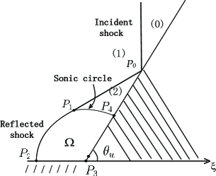
respectively, where $u_{1}=\sqrt{\frac{2(\rho_{1}-\rho_{0})(\rho_{1}^{\gamma-1}-\rho_{0}^{\gamma-1})}{(\gamma-1)(\rho_{1}+\rho_{0})}}>0$ and $\xi_{0}=\frac{\rho_{1}u_{1}}{\rho_{1}-\rho_{0}}>0$ are the velocity of state (1) and the location of the incident shock-front, uniquely determined by $(\rho_{0},\rho_{1},\gamma)$ through (6.8). Then $P_{0}=(\xi_{0},\xi_{0}\tan\theta_{w})$ in Fig. 2, and Problem 6.2 in the context of the potential flow equation can be formulated as

Problem 6.3 (Boundary value problem) (cf. Fig. 2). Seek a solution $\varphi$ of (6.6) in the self-similar domain $\Lambda$ with the boundary condition on $\partial\Lambda$:

$$\nabla\varphi\cdot{\bf n}|_{\partial\Lambda}=0,$$ (6.11)

and the asymptotic boundary condition at infinity:

$$\varphi\to\bar{\varphi}:=\begin{cases}\varphi_{0}\qquad\mbox{for}\,\,\,\xi>\xi_{0},\eta>\xi\tan\theta_{w},\\ \varphi_{1}\qquad\mbox{for}\,\,\,\xi<\xi_{0},\eta>0,\end{cases}\qquad\mbox{when $\xi^{2}+\eta^{2}\to\infty$},$$ (6.12)

where (6.12) holds in the sense that $\displaystyle\lim_{R\to\infty}\|\varphi-\overline{\varphi}\|_{C(\Lambda\setminus B_{R}(0))}=0.$

In Chen-Feldman [49], we first followed the von Neumann criterion and the stability criterion introduced above to establish a local existence theory of regular shock reflection near the reflection point $P_{0}$ in the level of potential flow, when the wedge angle is large and close to $\frac{\pi}{2}$. In this case, the vertical line is the incident shock-front that hits the wedge at $P_{0}=(\xi_{0},\xi_{0}\tan\theta_{w})$, and state (0) and state (1) ahead of and behind $S$ are given by $\varphi_{0}$ and $\varphi_{1}$ defined in (6.9) and (6.10), respectively. The solutions $\varphi$ and $\varphi_{1}$ differ only in the domain $P_{0}{P_{1}}{P_{2}}{P_{3}}$ because of shock diffraction by the wedge, where the curve $P_{0}{P_{1}}{P_{2}}$ is the reflected shock-front with the straight segment $P_{0}{P_{1}}$. State (2) behind $P_{0}{P_{1}}$ can be computed explicitly with the form:

$$\varphi_{2}(\xi,\eta)=-\frac{1}{2}(\xi^{2}+\eta^{2})+u_{2}(\xi-\xi_{0})+(\eta-\xi_{0}\tan\theta_{w})u_{2}\tan\theta_{w},$$ (6.13)

which satisfies $\nabla\varphi\cdot{\bf n}=0$ on $\partial\Lambda\cap\{\xi>0\}$; the constant velocity $u_{2}$ and the angle $\theta_{s}$ between $P_{0}{P_{1}}$ and the $\xi$–axis are determined by $(\theta_{w},\rho_{0},\rho_{1},\gamma)$ from the two algebraic equations expressing (6.8) and continuous matching of states (1) and (2) across $P_{0}{P_{1}}$ as in Theorem 6.1. Moreover, $\varphi_{2}$ is the unique solution in the domain $P_{0}{P_{1}}{P_{4}}$, as argued in [34, 183]. Hence $P_{1}P_{4}:=\Gamma_{sonic}=\partial\Omega\cap\partial B_{c_{2}}(u_{2},u_{2}\tan\theta_{w})$ is the sonic arc of state $(2)$ with center $(u_{2},u_{2}\tan\theta_{w})$ and radius $c_{2}$.

It should be noted that, in order that the solution $\varphi$ in the domain $\Omega$ is a part of the global solution to Problem 6.3, that is, $\varphi$ satisfies the equation in the sense of distributions in $\Lambda$, especially across the sonic arc $P_{1}P_{4}$, it is required that $\nabla(\varphi-\varphi_{2})\cdot{\bf n}|_{P_{1}P_{4}}=0.$ That is, we have to match our solution with state (2), which is the necessary condition for our solution in the domain $\Omega$ to be a part of the global solution. To achieve this, we have to show that our solution is at least $C^{1}$ with $\nabla(\varphi-\varphi_{2})=0$ across $P_{1}P_{4}$. Then Problem 6.3 can be reformulated as the following free boundary problem:

Problem 6.4 (Free boundary problem). Seek a solution $\varphi$ and a free boundary $P_{1}P_{2}=\{\xi=f(\eta)\}$ such that

• $f\in C^{1,\alpha}$ and

  $$\Omega:=\{\xi>f(\eta)\}\cap\Lambda{=\{\varphi<\varphi_{1}\}\cap\Lambda};$$ (6.14)

• $\varphi$ satisfies the free boundary condition (6.8) along $P_{1}P_{2}$;

• $\varphi\in C^{1,\alpha}(\overline{\Omega})\cap C^{2}(\Omega)$ solves (6.6) in $\Omega$, is subsonic in $\Omega$, and satisfies

  $$(\varphi-\varphi_{2},\nabla(\varphi-\varphi_{2})\cdot{\bf n})|_{P_{1}P_{2}}=0,$$ (6.15)

  $$\nabla\varphi\cdot{\bf n}|_{P_{3}P_{4}\cup\Gamma_{symm}}=0.$$ (6.16)

The boundary condition on $\Gamma_{symm}$ implies that $f^{\prime}(0)=0$ and thus ensures the orthogonality of the free boundary with the $\xi$-axis. Formulation (6.14) implies that the free boundary is determined by the level set $\varphi=\varphi_{1}$. The free boundary condition (6.8) along $P_{1}P_{2}$ is the conormal boundary condition on $P_{1}P_{2}$. Condition (6.15) ensures that the solution of the free boundary problem in $\Omega$ is a part of the global solution. Condition (6.16) is the slip boundary condition. Problem 6.4 involves two types of transonic flow: one is a continuous transition through the sonic arc $P_{1}P_{4}$ as a fixed boundary from the supersonic region (2) to the subsonic region $\Omega$; the other is a jump transition through the transonic shock-front as a free boundary from the supersonic region (1) to the subsonic region $\Omega$.

In Chen-Feldman [49, 50, 51], we have developed a rigorous mathematical approach to solve the von Neumann sonic conjecture, Problem 6.4, and established a global theory for solutions of regular reflection-diffraction up to the sonic angle, which converge to the unique solution of the normal shock reflection when $\theta_{w}$ tends to ${\pi}/{2}$. For more details, see Chen-Feldman [49, 50, 51].

The mathematical existence of Mach reflection-diffraction configurations is still open; see [13, 74, 84]. Some progress has been made in the recent years in the study of the 2-D Riemann problem for hyperbolic conservation laws; see [35, 36, 39, 114, 115, 116, 122, 134, 140, 143, 144, 182, 184, 186, 188, 194, 213, 214] and the references cited therein.

Some recent developments in the study of the local nonlinear stability of multidimensional compressible vortex sheets can be found in Coulombel-Secchi [83], Bolkhin-Trakhinin [20], Trakhinin [200], Chen-Wang [68], and the references cited therein. Also see Artola-Majda [7]. For the construction of the non-self-similar global solutions for some multidimensional systems, see Chen-Wang-Yang [67] and the references cited therein.

7. Divergence-Measure Vector Fields and Multidimensional Conservation Laws

Naturally, we want to approach the questions of existence, stability, uniqueness, and long-time behavior of entropy solutions for M-D hyperbolic conservation laws with neither specific reference to any particular method for constructing the solutions nor additional regularity assumptions. Some recent efforts have been in developing a theory of divergence-measure fields to construct a global framework for the analysis of solutions of M-D hyperbolic systems of conservation laws.

Consider system (1.1) in ${\mathbb{R}}^{d}$. As discussed in §2.5, the $BV$ bound generically fails for the M-D case. In general, for M-D conservation laws, especially the Euler equations, solutions of (1.1) are expected to be in the following class of entropy solutions:

1. ${\bf u}(t,{\bf x})\in{\mathcal{M}}({\mathbb{R}}_{+}^{d+1})$, or $L^{p}({\mathbb{R}}_{+}^{d+1}),\,1\leq p\leq\infty$;

2. ${\bf u}(t,{\bf x})$ satisfies the Lax entropy inequality:

   $$\mu_{\eta}:=\partial_{t}\eta({\bf u}(t,{\bf x}))+\nabla_{\bf x}\cdot{\bf q}({\bf u}(t,{\bf x}))\leq 0$$ (7.1)

   in the sense of distributions for any convex entropy pair $(\eta,{\bf q}):{\mathbb{R}}^{n}\to{\mathbb{R}}\times{\mathbb{R}}^{d}$ so that $\eta({\bf u}(t,{\bf x}))$ and ${\bf q}({\bf u}(t,{\bf x}))$ are distributions.

The Schwartz Lemma infers from (7.1) that the distribution $\mu_{\eta}$ is in fact a Radon measure: $\hbox{div}_{(t,{\bf x})}(\eta({\bf u}(t,{\bf x})),{\bf q}({\bf u}(t,{\bf x})))\in{\mathcal{M}}({\mathbb{R}}_{+}^{d+1}).$ Furthermore, when ${\bf u}\in L^{\infty}$, this is also true for any $C^{2}$ entropy-entropy flux pair $(\eta,{\bf q})$ ($\eta$ not necessarily convex) if (1.1) has a strictly convex entropy, which was first observed in Chen [38]. More generally, we have

Definition. Let ${\mathcal{D}}\subset{{\mathbb{R}}}^{N}$ be open. For $1\leq p\leq\infty$, ${\bf F}$ is called a ${\mathcal{D}M}^{p}({\mathcal{D}})$–field if ${\bf F}\in L^{p}({\mathcal{D}};{{\mathbb{R}}}^{N})$ and

$$\|{\bf F}\|_{{\mathcal{D}M}^{p}({\mathcal{D}})}:=\|{\bf F}\|_{L^{p}({\mathcal{D}};{\mathbb{R}}^{N})}+\|\hbox{div}{\bf F}\|_{{\mathcal{M}}({\mathcal{D}})}<\infty;$$ (7.2)

and the field ${\bf F}$ is called a ${{\mathcal{D}M}}^{ext}({\mathcal{D}})$–field if ${\bf F}\in{\mathcal{M}}({\mathcal{D}};{\mathbb{R}}^{N})$ and

$$\|{\bf F}\|_{{\mathcal{D}M}^{ext}({\mathcal{D}})}:=\|({\bf F},\hbox{div}{\bf F})\|_{{\mathcal{M}}({\mathcal{D}})}<\infty.$$ (7.3)

Furthermore, for any bounded open set ${\mathcal{D}}\subset{{\mathbb{R}}}^{N}$, ${\bf F}$ is called a ${{\mathcal{D}M}}^{p}_{loc}({{\mathbb{R}}}^{N})$–field if ${\bf F}\in{{\mathcal{D}M}}^{p}({\mathcal{D}})$; and ${\bf F}$ is called a ${{\mathcal{D}M}}^{ext}_{loc}({{\mathbb{R}}}^{N})$–field if ${\bf F}\in{{\mathcal{D}M}}^{ext}({\mathcal{D}})$. A field ${\bf F}$ is simply called a ${\mathcal{D}M}$–field in ${\mathcal{D}}$ if ${\bf F}\in{\mathcal{D}M}^{p}({\mathcal{D}}),1\leq p\leq\infty$, or ${\bf F}\in{\mathcal{D}M}^{ext}({\mathcal{D}})$.

It is easy to check that these spaces, under the respective norms $\|{\bf F}\|_{{\mathcal{D}M}^{p}({\mathcal{D}})}$ and $\|{\bf F}\|_{{\mathcal{D}M}^{ext}({\mathcal{D}})}$, are Banach spaces. These spaces are larger than the space of $BV$-fields. The establishment of the Gauss-Green theorem, traces, and other properties of $BV$ functions in the 1950s (cf. Federer [105]; also Ambrosio-Fusco-Pallara [5], Giusti [112], and Volpert [203]) has significantly advanced our understanding of solutions of nonlinear PDEs and related problems in the calculus of variations, differential geometry, and other areas, especially for the 1-D theory of hyperbolic conservation laws. A natural question is whether the ${\mathcal{D}M}$–fields have similar properties, especially the normal traces and the Gauss-Green formula to deal with entropy solutions for M-D conservation laws.

On the other hand, motivated by various nonlinear problems from conservation laws, as well as for rigorous derivation of systems of balance laws with measure source terms from the physical principle of balance law and the recovery of Cauchy entropy flux through the Lax entropy inequality for entropy solutions of hyperbolic conservation laws by capturing the entropy dissipation, a suitable notion of normal traces and corresponding Gauss-Green formula for divergence-measure fields are required.

Some earlier efforts were made on generalizing the Gauss-Green theorem for some special situations, and relevant results can be found in Anzellotti [6] for an abstract formulation for ${\bf F}\in L^{\infty}$, Rodrigues [178] for ${\bf F}\in L^{2}$, and Ziemer [216] for a related problem for $\hbox{div}{\bf F}\in L^{1}$; also see Baiocchi-Capelo [10] and Brezzi-Fortin [29]. In Chen-Frid [54], an explicit way to calculate the suitable normal traces was first observed for ${\bf F}\in{\mathcal{D}M}^{\infty}$, under which a generalized Gauss-Green theorem was shown to hold, which has motivated the development of a theory of divergence-measure fields in [54, 64, 66].

Some entropy methods based on the theory of divergence-measure fields presented above have been developed and applied for solving various nonlinear problems for hyperbolic conservation laws and related nonlinear PDEs. These problems especially include (i) Stability of Riemann solutions, which may contain rarefaction waves, contact discontinuities, and/or vacuum states, in the class of entropy solutions of the Euler equations in [42, 54, 55]; (ii) Decay of periodic entropy solutions in [52]; (iii) Initial and boundary layer problems in [54, 60, 64, 202]; (iv) Rigorous derivation of systems of balance laws from the physical principle of balance law and the recovery of Cauchy entropy flux through the Lax entropy inequality for entropy solutions of hyperbolic conservation laws by capturing the entropy dissipation in [66];

It would be interesting to develop further the theory of divergence-measure fields and more efficient entropy methods for solving more various problems in PDEs and related areas whose solutions are only measures or $L^{p}$ functions. For more details, see [54, 64, 66].

We also refer the reader to the related papers on other aspects of multidimensional conservation laws in this volume.

Acknowledgements. The work of Gui-Qiang G. Chen was supported in part by NSF grants DMS-0935967, DMS-0807551, the Royal Society–Wolfson Research Merit Award (UK), and the EPSRC Science and Innovation award to the Oxford Centre for Nonlinear PDE (EP/E035027/1).

References

- [1] S. Alinhac, Existence of rarefaction waves for multidimensional hyperbolic quasilinear systems, Comm. Partial Diff. Eqs. 14 (1989), pp. 173–230.
- [2] H. W. Alt and L. A. Caffarelli, Existence and regularity for a minimum problem with free boundary, J. Reine Angew. Math. 325 (1981), pp. 105–144.
- [3] H. W. Alt, L. A. Caffarelli, and A. Friedman, A free-boundary problem for quasilinear elliptic equations, Ann. Scuola Norm. Sup. Pisa Cl. Sci. (4), 11 (1984), pp. 1–44.
- [4] L. Ambrosio and C. De Lellis, Existence of solutions for a class of hyperbolic systems of conservation laws in several space dimensions, Int. Math. Res. Not. 2003 (2003), pp. 2205–2220.
- [5] L. Ambrosio, N. Fusco, and D. Pallara, Functions of Bounded Variation and Free Discontinuity Problems, Oxford Mathematical Monographs, The Clarendon Press, Oxford University Press: New York, 2000.
- [6] G. Anzellotti, Pairings between measures and bounded functions and compensated compactness, Ann. Mat. Pura Appl. (4) 135 (1983), pp. 293–318.
- [7] M. Artola and A. Majda, Nonlinear development of instabilities in supersonic vortex sheets, I: the basic kink modes, Phys. D. 28 (1987), pp. 253–281; II: Resonant interaction among kink modes, SIAM J. Appl. Math. 49 (1989), pp. 1310–1349; Nonlinear kink modes for supersonic vortex sheets, Phys. Fluids A, 1 (1989), pp. 583–596.
- [8] M.-J. Bae, G.-Q. Chen, and M. Feldman, Regularity of solutions to regular shock reflection for potential flow, Invent. Math. 175 (2009), pp. 505–543.
- [9] M.-J. Bae and M. Feldman, Transonic shocks in multidimensional divergent nozzles, Preprint, 2010.
- [10] C. Baiocchi and A. Capelo, Variational and Quasi-Variational Inequalities, Applications to Free-Boundary Problems, Vols. 1,2, John Wiley: New York, 1984.
- [11] J. M. Ball, Convexity conditions and existence theorems in nonlinear elasticity, Arch. Ration. Mech. Anal. 63 (1977), pp. 337–403.
- [12] J. M. Ball, A version of the fundamental theorem for Young measures, In: PDEs and Continuum Models of Phase Transitions (Nice, 1988), Lecture Notes in Phys. 344 (1989), pp. 207–215, Springer-Verlag: Berlin-New York.
- [13] G. Ben-Dor, Shock Wave Reflection Phenomena, 2nd Edition, Springer-Verlag: New York, 2007.
- [14] S. Benzoni-Gavage and D. Serre, Multidimensional Hyperbolic Partial Differential Equations. First-Order Systems and Applications, The Clarendon Press and Oxford University Press: Oxford, 2007.
- [15] L. Bers, Existence and uniqueness of subsonic flows past a given profile, Comm. Pure Appl. Math. 7 (1954), pp. 441–504.
- [16] L. Bers, Mathematical Aspects of Subsonic and Transonic Gas Dynamics, John Wiley & Sons, Inc.: New York; Chapman & Hall, Ltd.: London 1958.
- [17] H. Berestycki, L. Caffarelli, and L. Nirenberg, Uniform estimates for regularization of free boundary problems, In: Analysis and Partial Differential Equations, pp. 567–619, Dekker: New York, 1990.
- [18] S. Bianchini and A. Bressan, Vanshing viscosity solutions of nonlinear hyperbolic systems, Ann. Math. (2), 161 (2005), 223–342.
- [19] W. Bleakney and A. H. Taub, Interaction of shock waves, Rev. Modern Phys. 21 (1949), pp. 584–605.
- [20] A. Blokhin, and Y. Trakhinin, Stability of strong discontinuities in fluids and MHD, In: Handbook of Mathematical Fluid Dynamics, Vol. 1, pp. 545–652, Elsevier Science B. V.: Amsterdam, The Netherlands, 2002.
- [21] G. Boillat, La Propagation des Ondes, Gauthier-Villars: Paris, 1965.
- [22] G. Boillat, Chocs caractéristiques, C. R. Acad. Sci. Paris Sér. A-B, 274A (1972), pp. 1018–1021; Involutions des systèmes conservatifs, C. R. Acad. Sci. Paris, Sèrie I, 307 (1988), pp. 891–894.
- [23] F. Bouchut, On zero pressure gas dynamics, In: Advances in Kinetic Theory and Computing, pp. 171–190, World Sci. Publishing: River Edge, NJ, 1994.
- [24] Y. Brenier, Hydrodynamic structure of the augmented Born–Infeld equations, Arch. Ration. Mech. Anal. 172 (2004), pp. 65–91.
- [25] Y. Brenier and E. Grenier, Sticky particles and scalar conservation laws, SIAM J. Numer. Anal. 35 (1998), pp. 2317–2328.
- [26] P. Brenner, The Cauchy problem for the symmetric hyperbolic systems in , Math. Scand. 19 (1966), pp. 27–37.
- [27] A. Bressan, Hyperbolic Systems of Conservation Laws: The One Dimensional Cauchy Problem, Oxford University Press: Oxford, 2000.
- [28] A. Bressan, An ill-posed Cauchy problem for a hyperbolic system in two space dimensions, Rend. Sem. Mat. Univ. Padova, 110 (2003), pp. 103–117.
- [29] F. Brezzi and M. Fortin, Mixed and Hydrid Finite Element Methods, Springer-Verlag: New York, 1991.
- [30] L. A. Caffarelli, A Harnack inequality approach to the regularity of free boundaries, I. Lipschitz free boundaries are , Rev. Mat. Iberoamericana, 3 (1987), pp. 139–162; II. Flat free boundaries are Lipschitz, Comm. Pure Appl. Math. 42 (1989), pp. 55–78; III. Existence theory, compactness, and dependence on , Ann. Scuola Norm. Sup. Pisa Cl. Sci. (4), 15 (1989), pp. 583–602.
- [31] S. Canić, B. L. Keyfitz, and G. Lieberman, A proof of existence of perturbed steady transonic shocks via a free boundary problem, Comm. Pure Appl. Math. 53 (2000), pp. 484–511.
- [32] S. Canić, B. L. Keyfitz, and E. H. Kim, Free boundary problems for nonlinear wave systems: Mach stems for interacting shocks, SIAM J. Math. Anal. 37 (2006), 1947–1977.
- [33] S. Canić, B. L. Keyfitz, and E. H. Kim, Free boundary problems for a quasilinear degenerate elliptic equation: regular reflection of weak shocks, Comm. Pure Appl. Math. 55 (2002), pp. 71–92.
- [34] T. Chang and G.-Q. Chen, Diffraction of planar shock along the compressive corner, Acta Math. Sci. 6 (1986), pp. 241–257.
- [35] T. Chang, G.-Q. Chen, and S. Yang, On the Riemann Problem for two-dimensional Euler equations I: Interaction of shocks and rarefaction waves; II: Interaction of contact discontinuities, Discrete Contin. Dynam. Systems, 1 (1995), pp. 555–584; 6 (2000), pp. 419–430.
- [36] T. Chang and L. Hsiao, The Riemann Problem and Interaction of Waves in Gas Dynamics, Longman Scientific & Technical, Harlow; and John Wiley & Sons, Inc.: New York, 1989.
- [37] J. -Y. Chemin, Dynamique des gaz à masse totale finie, Asymptotic Anal. 3 (1990), pp. 215–220.
- [38] G.-Q. Chen, Hyperbolic systems of conservation laws with a symmetry, Commun. Partial Diff. Eqs. 16 (1991), pp. 1461–1487.
- [39] G.-Q. Chen Euler Equations and Related Hyperbolic Conservation Laws, In: Handbook of Differential Equations: Evolutionary Differential Equations, Vol. 2, pp. 1–104, 2005, Elsevier Science B.V: Amsterdam, The Netherlands.
- [40] G.-Q. Chen, Remarks on global solutions to the compressible Euler equations with spherical symmetry, Proc. Royal Soc. Edinburgh, 127A (1997), pp. 243–259.
- [41] G.-Q. Chen, Vacuum states and stability of rarefaction waves for compressible flow, Meth. Appl. Anal. 7 (2000), pp. 337–362.
- [42] G.-Q. Chen and J. Chen, Vacuum states and global stability of rarefaction waves for the Euler equations for compressible fluids, J. Hyper. Diff. Eqns. 4 (2007), pp. 105–122.
- [43] G.-Q. Chen, J. Chen, and M. Feldman, Transonic shocks and free boundary problems for the full Euler equations in infinite nozzles, J. Math. Pures Appl. 88 (2007), pp. 191–218.
- [44] G.-Q. Chen, J. Chen, and M. Feldman, Existence and stability of transonic shocks in the full Euler flows past wedges, Preprint, August 2010.
- [45] G.-Q. Chen, C. M. Dafermos, M. Slemrod, and D. Wang On two-dimensional sonic-subsonic flow, Commun. Math. Phys. 271 (2007), pp. 635–647.
- [46] G.-Q. Chen and B. Fang, Stability of transonic shock-fronts in steady potential flow past a perturbed cone, Discrete Conti. Dynamical Systems, 23 (2009), pp. 85–114.
- [47] G.-Q. Chen and M. Feldman, Multidimensional transonic shocks and free boundary problems for nonlinear equations of mixed type, J. Amer. Math. Soc. 16 (2003), pp. 461–494; Steady transonic shocks and free boundary problems in infinite cylinders for the Euler equations, Comm. Pure Appl. Math. 57 (2004), pp. 310–356; Free boundary problems and transonic shocks for the Euler equations in unbounded domains, Ann. Scuola Norm. Sup. Pisa Cl. Sci. (5), 3 (2004), pp. 827–869.
- [48] G.-Q. Chen and M. Feldman, Existence and stability of multidimensional transonic flows through an infinite nozzle of arbitrary cross-sections, Arch. Ration. Mech. Anal. 184 (2007), pp. 185-242
- [49] G.-Q. Chen and M. Feldman, Potential theory for shock reflection by a large-angle wedge, Proceedings of the National Academy of Sciences USA (PNAS), 102 (2005), pp. 15368–15372; Global solutions to shock reflection by large-angle wedges for potential flow, Annals of Math. 171 (2010), 1067–1182.
- [50] G.-Q. Chen and M. Feldman, Shock reflection-diffraction and multidimensional conservation laws, In: Hyperbolic Problems: Theory, Numerics, and Applications, pp. 25–51, Proc. Sympos. Appl. Math. 67, AMS: Providence, RI, 2010.
- [51] G.-Q. Chen and M. Feldman, Shock reflection-diffraction and nonlinear partial differential equations of mixed type, Contemporary Mathematics, AMS: Providence (to appear); Potential Theory for Shock Reflection-Diffraction and von Neumann’s Conjectures, Preprint, July 2010.
- [52] G.-Q. Chen and H. Frid, Decay of entropy solutions of nonlinear conservation laws, Arch. Ration. Mech. Anal. 146 (1999), pp. 95–127; Large-time behavior of entropy solutions of conservation laws, J. Diff. Eqs. 152 (1999), pp. 308–357.
- [53] G.-Q. Chen and H. Frid, Large-time behavior of entropy solutions in for multidimensional conservation laws, In: Advances in Nonlinear PDE and Related Areas, pp. 28–44, World Scientific, Singapore, 1998.
- [54] G.-Q. Chen and H. Frid, Divergence-measure fields and hyperbolic conservation laws, Arch. Ration. Mech. Anal. 147 (1999), pp. 89–118; Extended divergence-measure fields and the Euler equations for gas dynamics, Commun. Math. Phys. 236 (2003), pp. 251–280.
- [55] G.-Q. Chen, H. Frid, and Y. Li, Uniqueness and stability of Riemann solutions with large oscillation in gas dynamics, Commun. Math. Phys. 228 (2002), pp. 201–217.
- [56] G.-Q. Chen and P.-T. Kan, Hyperbolic conservation laws with umbilic degeneracy (I)–(II): Arch. Ration. Mech. Anal. 130 (1995), pp. 231–276; 160 (2001), pp. 325–354.
- [57] G.-Q. Chen and P. LeFloch, Compressible Euler equations with general pressure law, Arch. Ration. Mech. Anal. 153 (2000), pp. 221–259; Existence theory for the isentropic Euler equations, Arch. Ration. Mech. Anal. 166 (2003), pp. 81–98.
- [58] G.-Q. Chen and T.-H. Li Well-posedness for two-dimensional steady supersonic Euler flows past a Lipschitz wedge, J. Diff. Eqs. 244 (2008), pp. 1521–1550.
- [59] G.-Q. Chen and H. Liu, Formation of delta-shocks and vacuum states in the vanishing pressure limit of solutions to the Euler equations for isentropic fluids, SIAM J. Math. Anal. 34 (2003), pp. 925–938; Concentration and cavitation in the vanishing pressure limit of solutions to the Euler equations for nonisentropic fluids, Phys. D, 189 (2004), pp. 141–165.
- [60] G.-Q. Chen and M. Rascle, Initial layers and uniqueness of weak entropy solutions to hyperbolic conservation laws, Arch. Ration. Mech. Anal. 153 (2000), pp. 205–220.
- [61] G.-Q. Chen, M. Slemrod, and D. Wang, Vanishing viscosity method for transonic flow, Arch. Ration. Mech. Anal. 189 (2008), pp. 159–188.
- [62] G.-Q. Chen, M. Slemrod, and D. Wang, Isometric immersion and compensated compactness, Commun. Math. Phys. 294 (2010), pp. 411–437.
- [63] G.-Q. Chen, M. Slemrod, and D. Wang, Weak continuity of the Gauss-Codazzi-Ricci equations for isometric embedding, Proc. Amer. Math. Soc. 138 (2010), pp. 1843–1852.
- [64] G.-Q. Chen and M. Torres, Divergence-measure fields, sets of finite perimeter, and conservation laws, Arch. Ration. Mech. Anal. 175 (2005), pp. 245–267.
- [65] G.-Q. Chen and M. Torres, On entropy solutions without bounded variation for hyperbolic systems of conservation laws, Preprint, 2010.
- [66] G.-Q. Chen, M. Torres, and W. Ziemer, Gauss-Green theorem for weakly differentiable fields, sets of finite perimeter, and balance laws, Comm. Pure Appl. Math. 62 (2009), pp. 242–304; Measure-theoretical analysis and nonlinear conservation laws, Pure Appl. Math. Quarterly, 3 (2007), pp. 841–879.
- [67] G.-Q. Chen, D.-H. Wang, and X.-Z. Yang, Evolution of discontinuity and formation of triple-shock pattern in solutions to a two-dimensional hyperbolic system of conservation laws, SIAM J. Math. Anal. 41 (2009), 1–25.
- [68] G.-Q. Chen and Y.-G. Wang, Existence and stability of compressible current-vortex sheets in three-dimensional magnetohydrodynamics, Arch. Ration. Mech. Anal. 187 (2007), pp. 369–408; Analysis of compressible current-vortex sheets in three-dimensional magnetohydrodynamics, Preprint, July 2010.
- [69] G.-Q. Chen, Y. Zhang, and D. Zhu, Existence and stability of supersonic Euler flows past Lipschitz wedges, Arch. Ration. Mech. Anal. 181 (2006), pp. 261–310.
- [70] G.-Q. Chen, Y. Zhang, and D. Zhu, Existence and stability of supersonic vortex sheets in Euler flows past Lipschitz walls, SIAM J. Math. Anal. 38 (2007), pp. 1660–1693.
- [71] S.-X. Chen, Existence of stationary supersonic flows past a point body, Arch. Ration. Mech. Anal. 156 (2001), pp. 141–181.
- [72] S.-X. Chen, Stability of transonic shock fronts in two-dimensional Euler systems, Trans. Amer. Math. Soc. 357 (2005), pp. 287–308; Transonic shocks in 3-D compressible flow passing a duct with a general section for Euler systems, Trans. Amer. Math. Soc. 360 (2008), pp. 5265–5289.
- [73] S.-X. Chen, Compressible flow and transonic shock in a diverging nozzle, Commun. Math. Phys. 289 (2009), pp. 75–106.
- [74] S.-X. Chen Stability of a Mach configuration, Comm. Pure Appl. Math. 59 (2006), pp. 1–35; Mach configuration in pseudo-stationary compressible flow, J. Amer. Math. Soc. 21 (2008), pp. 63–100.
- [75] S.-X. Chen and B. Fang, Stability of transonic shocks in supersonic flow past a wedge, J. Diff. Eqs. 233 (2007), pp. 105–135.
- [76] S.-X. Chen and H. Yuan, Transonic shocks in compressible flow passing a duct for three-dimensional Euler systems, Arch. Ration. Mech. Anal. 187 (2008), pp. 523–556.
- [77] S.-X. Chen, Z. Xin, and H. Yin, Global shock waves for the supersonic flow past a perturbed cone, Commun. Math. Phys. 228 (2002), pp. 47–84.
- [78] A. J. Chorin, Vorticity and Turbulence, Springer-Verlag: New York, 1994.
- [79] D. Christodoulou, The Formation of Shocks in 3-Dimensional Fluids, European Mathematical Society (EMS): Zürich, 2007.
- [80] D. Christodoulou, The Formation of Black Holes in General Relativity, European Mathematical Society (EMS): Zürich, 2009.
- [81] J. D. Cole and L. P. Cook, Transonic Aerodynamics, Elsevier: Amsterdam, 1986.
- [82] P. Constantin, Some mathematical problems of fluid mechanics, Proceedings of the International Congress of Mathematicians, Vols. 1–2 (Zürich, 1994), pp. 1086–1095, Birkhäuser: Basel, 1995.
- [83] J. F. Coulombel and P. Secchi, The stability of compressible vortex sheets in two space dimensions, Indiana Univ. Math. J. 53 (2004), 941–1012; Nonlinear compressible vortex sheets in two space dimensions, Ann. Sci. Éc. Norm. Supér. (4), 41 (2008), 85–139; Uniqueness of 2-D compressible vortex sheets, Commun. Pure Appl. Anal. 8 (2009), 1439–1450.
- [84] R. Courant and K. O. Friedrichs, Supersonic Flow and Shock Waves, Springer-Verlag: New York, 1962.
- [85] R. Courant and D. Hilbert, Methods of Mathematical Physics, Interscience Publishers, Inc.: New York, 1953.
- [86] M. S. Cramer and A. R. Seebass, Focusing of a weak shock at an arâte, J. Fluid Mech. 88 (1978), pp. 209–222.
- [87] D. Cui and H. Yin, Global supersonic conic shock wave for the steady supersonic flow past a cone: polytropic gas, J. Diff. Eqs. 246 (2009), pp. 641–669.
- [88] B. Dacorogna, Weak Continuity and Weak Lower Semicontinuity of Nonlinear Functionals, Lecture Notes in Math. 922, Springer-Verlag: New York, 1982.
- [89] C. M. Dafermos, Quasilinear hyperbolic systems with involutions, Arch. Ration. Mech. Anal. 94 (1986), 373–389.
- [90] C. M. Dafermos, Entropy and the stability of classical solutions of hyperbolic systems of conservation laws, Lecture Notes in Math. 1640, pp. 48–69, Springer-Verlag: Berlin, 1996.
- [91] C. M. Dafermos, Hyperbolic Conservation Laws in Continuum Physics, Springer-Verlag: Berlin, 2010.
- [92] C. De Lellis, F. Otto, and M. Westdickenberg, Structure of entropy solutions for multidimensional scalar conservation laws, Arch. Ration. Mech. Anal. 170 (2003), pp. 137–184.
- [93] C. De Leliss and L. Székelyhidi Jr. The Euler equations as a differential inclusion, Ann. of Math. (2), 170 (2009), 1417–1436; On admissibility criteria for weak solutions of the Euler equations, Arch. Ration. Mech. Anal. 195 (2010), 225–260.
- [94] S. Demoulini, D. M. Stuart, and A. E. Tzavaras, A variational approximation scheme for three-dimensional elastodynamics with polyconvex energy, Arch. Ration. Mech. Anal. 157 (2001), pp. 325–344.
- [95] R. J. DiPerna, Compensated compactness and general systems of conservation laws, Trans. Amer. Math. Soc. 292 (1985), pp. 383–420.
- [96] R. J. DiPerna, Convergence of approximate solutions to conservation laws, Arch. Ration. Mech. Anal. 88 (1985), pp. 223–270; Convergence of viscosity method for isentropic gas dynamics, Commun. Math. Phys. 91 (1983), pp. 1–30.
- [97] R. J. DiPerna, Measure-valued solutions to conservation laws, Arch. Ration. Mech. Anal. 88 (1985), 223–270.
- [98] G. Dong, Nonlinear Partial Differential Equations of Second Order, Transl. Math. Monographs, 95, AMS: Providence, RI, 1991.
- [99] W. E, Y. Rykov, and Y. Sinai, Generalized variational principles, global weak solutions, and behavior with random initial data for systems of conservation laws arising in adhesion particle dynamics, Commun. Math. Phys. 177 (1996), pp. 349–380.
- [100] V. Elling and T.-P. Liu, The ellipticity principle for self-similar potential flows, J. Hyperbolic Differential Equations, 2 (2005), 909–917.
- [101] V. Elling and T.-P. Liu, Supersonic flow onto a solid wedge, Comm. Pure Appl. Math. 61 (2008), pp. 1347–1448.
- [102] B. Engquist and W. E, Large time behavior and homogenization of solutions of two-dimensional conservation laws, Comm. Pure Appl. Math. 46 (1993), pp. 1–26.
- [103] L. C. Evans, Weak Convergence Methods for Nonlinear Partial Differential Equations, CBMS 72, AMS: Providence, RI, 1990.
- [104] B. Fang, Stability of transonic shocks for the full Euler system in supersonic flow past a wedge, Math. Methods Appl. Sci. 29 (2006), pp. 1–26.
- [105] H. Federer, Geometric Measure Theory, Springer-Verlag: Berlin-Heidelberg-New York, 1969.
- [106] R. Finn and D. Gilbarg, Three-dimensional subsonic flows, and asymptotic estimates for elliptic partial differential equations, Acta Math. 98 (1957), pp. 265–296.
- [107] S. Friedland, J. W. Robbin, and J. Sylvester, On the crossing rule, Comm. Pure Appl. Math. 37 (1984), pp. 19–38.
- [108] K. O. Friedrichs, Symmetric hyperbolic linear differential equations, Comm. Pure Appl. Math. 7 (1954), pp. 345–392.
- [109] K. Friedrichs and P. Lax, Systems of conservation laws with a convex extension, Proc. Nat. Acad. Sci., U.S.A. 68 (1971), pp. 1686–1688.
- [110] I. M. Gamba and C. S. Morawetz, A viscous approximation for a -D steady semiconductor or transonic gas dynamic flow: existence theorem for potential flow, Comm. Pure Appl. Math. 49 (1996), pp. 999–1049.
- [111] W. Gangbo and M. Westdickenberg, Optimal transport for the system of isentropic Euler equations, Comm. Partial Diff. Eqs. 34 (2009), 1041–1073.
- [112] E. Giusti, Minimal Surfaces and Functions of Bounded Variation, Birkhäuser Verlag: Basel, 1984.
- [113] J. Glimm, Solutions in the large for nonlinear hyperbolic system of equations, Comm. Pure Appl. Math. 18 (1965), pp. 95–105.
- [114] J. Glimm, X. Ji, J. Li, X. Li, P. Zhang, T. Zhang, and Y. Zheng, Transonic shock formation in a rarefaction Riemann problem for the 2D compressible Euler equations, SIAM J. Appl. Math. 69 (2008), pp. 720–742.
- [115] J. Glimm, C. Klingenberg, O. McBryan, B. Plohr, D. Sharp, and S. Yaniv, Front tracking and two-dimensional Riemann problems, Adv. Appl. Math. 6 (1985), pp. 259–290.
- [116] J. Glimm and A. Majda, Multidimensional Hyperbolic Problems and Computations, IMA Volumes in Mathematics and its Applications, 29, Springer-Verlag: New York, 1991.
- [117] S. Godunov, An interesting class of quasilinear systems, Dokl. Akad. Nauk SSSR. 139 (1961), pp. 521–523, English transl: Soviet Math. 2 (1961), pp. 947–949; Elements of Continuum Mechanics, Moscow: Nauka, 1978; Lois de conservation et integrals d’énergie des équations hyperboliques, Lecture Notes in Math. 1270 (1987), pp. 135–149, Berlin: Springer.
- [118] E. Grenier, Existence globale pour le système des gaz sans pression, C. R. Acad. Sci. Paris Sér. I Math. 321 (1995), pp. 171–174.
- [119] C.-H. Gu, A method for solving the supersonic flow past a curved wedge (in Chinese), Fudan Univ. J. 7 (1962), pp. 11–14.
- [120] O. Guès, G. Métiver, M. Williams, and K. Zumbrun, Navier-Stokes regularization of multidimensional Euler shocks, Ann. Sci. École Norm. Sup. (4) 39 (2006), pp. 75–175.
- [121] K. G. Guderley, The Theory of Transonic Flow, Pergamon Press: Oxford-London-Paris-Frankfurt; Addison-Wesley Publishing Co. Inc.: Reading, Mass. 1962.
- [122] L. Guo, W. Sheng, and T. Zhang, The two-dimensional Riemann problem for isentropic Chaplygin gas dynamic system, Commun. Pure Appl. Anal. 9 (2010), pp. 431–458.
- [123] J. Hadamard, Leçons sur la Propagation des Ondes et les Équations de l’Hydrodynamique, Hermann, Paris, 1903 (Reprinted by Chelsea 1949).
- [124] Q. Han and J.-X. Hong, Isometric embedding of Riemannian manifolds in Euclidean spaces, AMS: Providence, RI, 2006.
- [125] D. Hoff, The zero-Mach limit of compressible flows, Comm. Math. Phys. 192 (1998), pp. 543–554.
- [126] H. Holden and N. H. Risebro, Front Tracking for Hyperbolic Conservation Laws, Springer-Verlag: New York, 2002.
- [127] F. Huang and Z. Wang, Well posedness for pressureless flow, Commun. Math. Phys. 222 (2001), pp. 117–146.
- [128] J. Hunter, Transverse diffraction of nonlinear waves and singular rays, SIAM J. Appl. Math. 48 (1988), pp. 1–37; Nonlinear wave diffraction, In: Geometrical Optics and Related Topics (Cortona, 1996), pp. 221–243, Birkhäuser Boston: Boston, MA, 1997.
- [129] J. Hunter and J. Keller, Weak shock diffraction, Wave Motion, 6 (1984), pp. 79–89 and pp. 321.
- [130] H. K. Jenssen, Blowup for systems of conservation laws, SIAM J. Math. Anal. 31 (2000), pp. 894–908.
- [131] T. Kato, The Cauchy problem for quasi-linear symmetric hyperbolic systems, Arch. Ration. Mech. Anal. 58 (1975), pp. 181–205; Quasilinear equations of evolution with applications to partial differential equations, Lecture Notes in Math. 448, pp. 25–70, Springer-Verlag: Berlin, 1975.
- [132] J. B. Keller and A. Blank, Diffraction and reflection of pulses by wedges and corners, Comm. Pure Appl. Math. 4 (1951), pp. 75–94.
- [133] J. B. Keller and L. Ting, Periodic vibrations of systems governed by nonlinear partial differential equations, Comm. Pure Appl. Math. 19 (1966), pp. 371–420.
- [134] A. Kurganov and E. Tadmor, Solution of two-dimensional Riemann problems for gas dynamics without Riemann problem solvers, Numer. Methods Partial Diff. Eqs. 18 (2002), pp. 584–608.
- [135] A. G. Kuz’min, Boundary Value Problems for Transonic Flow, John Wiley & Sons, 2002.
- [136] P. D. Lax, Shock waves and entropy, In: Contributions to Nonlinear Functional Analysis, E. A. Zarantonello (ed.), pp. 603–634, Academic Press: New York, 1971.
- [137] P. D. Lax, Hyperbolic Systems of Conservation Laws and the Mathematical Theory of Shock Waves, SIAM: Philadelphia, 1973.
- [138] P. D. Lax, The multiplicity of eigenvalues, Bull. Amer. Math. Soc. (N.S.), 6 (1982), pp. 213–214.
- [139] P. D. Lax, Hyperbolic systems of conservation laws in several space variables, In: Current Topics in PDEs, pp. 327–341, Kinokuniya: Tokyo, 1986.
- [140] P. D. Lax and X.-D. Liu, Solutions of two dimensional Riemann problem of gas dynamics by positive schemes, SIAM J. Sci. Comput. 19 (1998), pp. 319–340.
- [141] P. G. LeFloch, Hyperbolic Systems of Conservation Laws : The theory of classical and nonclassical shock waves, Birkhäuser: Zürich, 2002.
- [142] J. Li, Note on the compressible Euler equations with zero temperature, Appl. Math. Lett. 14 (2001), pp. 519–523.
- [143] J. Li, T. Zhang, and S. Yang, The Two-Dimensional Riemann Problem in Gas Dynamics, Longman (Pitman Monographs 98): Essex, 1998.
- [144] J. Li and Y. Zheng, Interaction of four rarefaction waves in the bi-symmetric class of the two-dimensional Euler equations, Comm. Math. Phys. 296 (2010), pp. 303–321.
- [145] J. Li, Z. Xin, and H. Yin, On transonic shocks in a nozzle with variable end pressure, Commun. Math. Phys. 291 (2009), pp. 111–150.
- [146] T.-T. Li, On a free boundary problem, Chinese Ann. Math. 1 (1980), pp. 351–358.
- [147] T.-T. Li and W.-C. Yu, Boundary Value Problems for Quasilinear Hyperbolic Systems, Duke University Press: Durham, 1985.
- [148] M. J. Lighthill, The diffraction of a blast I, Proc. Royal Soc. London, 198 (1949), pp. 454–47; The diffraction of a blast II, Proc. Roy. Soc. London, 200A (1950), pp. 554–565.
- [149] W.-C. Lien and T.-P. Liu, Nonlinear stability of a self-similar 3-dimensional gas flow, Commun. Math. Phys. 204 (1999), pp. 525–549.
- [150] P.-L. Lions, Mathematical Topics in Fluid Mechanics, Vols. 1–2, Oxford University Press: Oxford, 1998.
- [151] P.-L. Lions and N. Masmoudi, Incompressible limit for a viscous compressible fluid, J. Math. Pures Appl. (9), 77 (1998), pp. 585–627.
- [152] P.-L. Lions, B. Perthame, and E. Tadmor, A kinetic formulation of multidimensional scalar conservation laws and related equations, J. Amer. Math. Soc. 7 (1994), pp. 169–191.
- [153] L. Liu and H. R. Yuan, Stability of cylindrical transonic shocks for two-dimensional steadt compressible Euler system, J. Hyper. Diff. Eqs. 5 (2008), pp. 347–379.
- [154] T.-P. Liu and T. Yang, stability of weak solutions for systems of hyperbolic conservation laws, J. Amer. Math. Soc. 12 (1999), pp. 729–774; Well-posedness theory for hyperbolic conservation laws, Comm. Pure Appl. Math. 52 (1999), pp. 1553–1586.
- [155] E. Mach, Über den verlauf von funkenwellenin der ebene und im raume, Sitzungsber. Akad. Wiss. Wien, 78 (1878), pp. 819–838.
- [156] A. Majda, The stability of multidimensional shock fronts, Mem. Amer. Math. Soc. 275, AMS: Providence, 1983; The existence of multidimensional shock fronts, Mem. Amer. Math. Soc. 281, AMS: Providence, 1983.
- [157] A. Majda, Compressible Fluid Flow and Systems of Conservation Laws in Several Space Variables, Springer-Verlag: New York, 1984.
- [158] A. Majda and A. Bertozzi, Vorticity and Incompressible Flow, Cambridge University Press: Cambridge, 2002.
- [159] A. Majda and E. Thomann, Multidimensional shock fronts for second order wave equations, Comm. Partial Diff. Eqs. 12 (1987), pp. 777–828.
- [160] T. Makino, S. Ukai, and S. Kawashima, Sur la solution à support compact de l’iquations d’Euler compressible, Japan J. Appl. Math. 3 (1986), pp. 249–257.
- [161] V. G. Maz’ya and B. A. Plamenevskivı, Estimates in and in Hölder classes and the Miranda-Agman maximun principle for solutions of elliptic boundary value problems in domains with sigular points on the boundary, Amer. Math. Soc. Transl., 123 (1984), pp. 1–56.
- [162] G. Métivier, Stability of multi-dimensional weak shocks, Comm. Partial Diff. Eqs. 15 (1990), pp. 983–1028.
- [163] C. S. Morawetz, On a weak solution for a transonic flow problem, Comm. Pure Appl. Math. 38 (1985), pp. 797–818. On steady transonic flow by compensated compactness, Meth. Appl. Anal. 2 (1995), pp. 257–268.
- [164] C. S. Morawetz, Mixed equations and transonic flow, J. Hyper. Diff. Eqns. 1 (2004), pp. 1–26.
- [165] C. S. Morawetz, Potential theory for regular and Mach reflection of a shock at a wedge, Comm. Pure Appl. Math. 47 (1994), pp. 593–624.
- [166] C. S. Morawetz, On the non-existence of continuous transonic flows past profiles I,II,III, Comm. Pure Appl. Math. 9 (1956), pp. 45–68; 10 (1957), pp. 107–131; 11 (1958), pp. 129–144.
- [167] C. B. Morrey, Quasiconvexity and the lower semicontinuity of multiple integrals, Pacific J. Math. 2 (1952), pp. 25–53.
- [168] F. Murat, The injection of the positive cone of in is completely continuous for all , J. Math. Pures Appl. (9), 60 (1981), pp. 309–322.
- [169] F. Murat, Compacité par compensation, Ann. Suola Norm. Pisa (4), 5 (1978), pp. 489–507; Compacité par compensation, condition nécessaire et suffisante de continuité faible sous une hypothèse de range constant, Ann. Scuola Norm. Sup. Pisa (4), 8 (1981), pp. 69–102; A survey on compensated compactness, In: Contributions to Modern Calculus of Variations (Bologna, 1985), pp. 145–183, Longman Sci. Tech.: Harlow, 1987.
- [170] J. von Neumann, Oblique reflection of shocks, Navy Department, Bureau of Ordance, Explosive Research Report, No. 12, 1943.
- [171] J. von Neumann, Collect Works, Vol. 5, Pergamon: New York, 1963.
- [172] S. Osher, M. Hafez, and W. Whitlow, Entropy condition satisfying approximations for the full potential equation of transonic flow, Math. Comp. 44 (1985), pp. 1–29.
- [173] E. Yu. Panov, Existence of strong traces for quasi-solutions of multidimensional conservation laws, J. Hyper. Diff. Eqs. 4 (2007), pp. 729–770.
- [174] B. Perthame, Time decays: an analogy between kinetic transport, Schrödinger and gas dynamics equations, In: Nonlinear Partial Differential Equations and Their Applications, pp. 281–293, Longman: Harlow, 1998.
- [175] B. Perthame, Kinetic Formations of Conservation Laws, Oxford University Press: Oxford, 2002.
- [176] T. Qin, Symmetrizing the nonlinear elastodynamic system, J. Elasticity, 50 (1998), pp. 245–252.
- [177] J. Rauch, estimates fail for most quasilinear hyperbolic systems in dimension great than one, Commun. Math. Phys. 106 (1986), pp. 481–484.
- [178] J.-F. Rodrigues, Obstacle Problems in Mathematical Physics, Elsevier Science Publishers B.V. 1987.
- [179] T. Ruggeri and A. Strumia, Main field and convex covariant density for quasilinear hyperbolic systems, Ann. Inst. Henri Poincaré, Section A, 34 (1981), pp. 65–84.
- [180] D. G. Schaeffer, Supersonic flow past a nearly straight wedge, Duke Math. J. 43 (1976), pp. 637–670.
- [181] D. Schaeffer and M. Shearer, The classification of systems of nonstrictly hyperbolic conservation laws, with application to oil recovery, Comm. Pure Appl. Math. 40 (1987), pp. 141–178; Riemann problems for nonstrictly hyperbolic systems of conservation laws, Trans. Amer. Math. Soc. 304 (1987), pp. 267–306.
- [182] C. W. Schulz-Rinne, J. P. Collins, and H. M. Glaz, Numerical solution of the Riemann problem for two-dimensional gas dynamics, SIAM J. Sci. Comput. 14 (1993), pp. 1394–1414.
- [183] D. Serre, Écoulements de fluides parfaits en deux variables indépendantes de type espace. Rèflexion d’un choc plan par un dièdre compressif (French), Arch. Ration. Mech. Anal. 132 (1995), pp. 15–36.
- [184] D. Serre, Spiral waves for the two-dimensional Riemann problem for a compressible fluid, Ann. Fac. Sci. Toulouse Math. (6), 5 (1996), pp. 125–135.
- [185] D. Serre, Hyperbolicity of the nonlinear models of Maxwell’s equations, Arch. Ration. Mech. Anal. 172 (2004), pp. 309–331.
- [186] D. Serre, Multidimensional shock interaction for a Chaplygin gas, Arch. Ration. Mech. Anal. 191 (2009), pp. 539–577.
- [187] W.-C. Sheng and G. Yin, Transonic shock and supersonic shock in the regular reflection of a planar shock, Z. Angew. Math. Phys. 60 (2009), pp. 438–449.
- [188] W.-C. Sheng and T. Zhang, The Riemann Problem for the Transportation Equations in Gas Dynamics, Mem. Amer. Math. Soc. 654, AMS: Providence, 1999.
- [189] M. Shiffman, On the existence of subsonic flows of a compressible fluid, J. Ration. Mech. Anal. 1 (1952), pp. 605–652.
- [190] T. C. Sideris, Formation of singularities in three-dimensional compressible fluids, Commun. Math. Phys. 101 (1985), pp. 475–485.
- [191] B. Skews and J. Ashworth, The physical nature of weak shock wave reflection, J. Fluid Mech. 542 (2005), pp. 105–114.
- [192] E. Tabak and R. Rosales, Focusing of weak shock waves and the von Neumann paradox of oblique shock reflection, Phys. Fluids, 6 (1994), pp. 1874–1892.
- [193] E. Tadmor, M. Rascle, and P. Bagnerini, Compensated compactness for 2D conservation laws, J. Hyperbolic Differ. Equ. 2 (2005), 697–712.
- [194] D. Tan and T. Zhang, Two dimensional Riemann problem for a hyperbolic system of nonlinear conservation laws I: four-J cases, J. Diff. Eqs. 111 (1994), pp. 203–254; II: Initial data involving some rarefaction waves, J. Diff. Eqs. 111 (1994), pp. 255–283.
- [195] L. Tartar, Compensated compactness and applications to partial differential equations. In: Res. Notes in Math. 39, pp. 136–212, Pitman: Boston-London, 1979.
- [196] L. Tartar, Une nouvelle méthode de resolution d’equations aux derivées partielles nonlinéaires, Lecture Notes in Math. 665, pp. 228–241, Springer-Verlag: Berlin, 1977; The compensated compactness method applied to systems of conservation laws, In: Systems of Nonlinear P.D.E., J. M. Ball (eds.), pp. 263–285, NATO Series, C. Reidel publishing Co. 1983.
- [197] A. Tesdall and J. K. Hunter, Self-similar solutions for weak shock reflection, SIAM J. Appl. Math. 63 (2002), pp. 42–61.
- [198] A. M. Tesdall, R. Sanders, and B. Keyfitz, Self-similar solutions for the triple point paradox in gasdynamics, SIAM J. Appl. Math. 68 (2008), pp. 1360–1377.
- [199] R. Timman, Unsteady motion in transonic flow, In: Symposium Transsonicum (IUTAM, Aachen, Sept. 1962), pp. 394–401, ed. K. Oswatitsch, Springer-Verlag: Berlin, 1964.
- [200] Y. Trakhinin, Existence of compressible current-vortex sheets: variable coefficients linear analysis, Arch. Ration. Mech. Anal. 177 (2005), 331–366; The existence of current-vortex sheets in ideal compressible magnetohydrodynamics, Arch. Ration. Mech. Anal. 191 (2009), 245–310.
- [201] M. Van Dyke, An Album of Fluid Motion, The Parabolic Press: Stanford, 1982.
- [202] A. Vasseur, Strong traces for solutions to multidimensional scalar conservation laws, Arch. Ration. Mech. Anal. 160 (2001), 181–193.
- [203] A. Volpert, The Space and quasilinear equations, Mat. Sb. (N.S.) 73 (1967), 255–302; Math. USSR Sbornik, 2 (1967), 225–267 (in English).
- [204] Z. Wang, F. Huang, and X. Ding, On the Cauchy problem of transportation equations, Acta Math. Appl. Sinica (English Ser.), 13 (1997), pp. 113–122.
- [205] G. B. Whitham, Linear and Nonlinear Waves, Wiley-Interscience: New York, 1973.
- [206] Z. Xin, W. Yan, and H. Yin, Transonic shock problem for the Euler system in a nozzle, Arch. Ration. Mech. Anal. 194 (2009), 1–47.
- [207] S.-T. Yau, Review of geometry and analysis, In: Mathematics: Frontiers and Perspectives, pp. 353–401, International Mathematics Union, Eds. V. Arnold, M. Atiyah, P. Lax, and B. Mazur, AMS: Providence, 2000.
- [208] G. I. Zabolotskaya and R. V. Khokhlov, Quasi-plane waves in the nonlinear acoustics of confined beams, Sov. Phys.-Acoustics, 15 (1969), pp. 35–40.
- [209] A. R. Zakharian, M. Brio, J. K. Hunter, and G. M. Webb, The von Neumann paradox in weak shock reflection, J. Fluid Mech. 422 (2000), pp. 193–205.
- [210] Ya. B. Zeldovich, Gravitational instability: an approximate theory for large density perturbations, Astronaut. Astrophys. 5 (1970), pp. 84–89.
- [211] T. Zhang and Y. Zheng, Conjecture on the structure of solutions of the Riemann problem for two-dimensional gas dynamics, SIAM J. Math. Anal. 21 (1990), pp. 593–630.
- [212] Y.-Q. Zhang, Global existence of steady supersonic potential flow past a curved wedge with a piecewise smooth boundary, SIAM J. Math. Anal. 31 (1999), pp. 166–183; Steady supersonic flow past an almost straight wedge with large vertex angle, J. Diff. Eqs. 192 (2003), pp. 1–46.
- [213] Y. Zheng, Systems of Conservation Laws: Two-Dimensional Riemann Problems, Birkhäuser: Boston, 2001.
- [214] Y. Zheng, A global solution to a two-dimensional Riemann problem involving shocks as free boundaries, Acta Math. Appl. Sin. Engl. Ser. 19 (2003), pp. 559–572.
- [215] Y. Zheng, Two-dimensional regular shock reflection for the pressure gradient system of conservation laws, Acta Math. Appl. Sin. Engl. Ser. 22 (2006), pp. 177–210.
- [216] W. P. Ziemer, Cauchy flux and sets of finite perimeter, Arch. Ration. Mech. Anal. 84 (1983), pp. 189–201.