Exact Path-Integral Representations for the $T$-Matrix in Nonrelativistic Potential Scattering

Abstract

Several path integral representations for the $T$-matrix in nonrelativistic potential scattering are given which produce the complete Born series when expanded to all orders and the eikonal approximation if the quantum fluctuations are suppressed. They are obtained with the help of “phantom” degrees of freedom which take away explicit phases that diverge for asymptotic times. Energy conservation is enforced by imposing a Faddeev-Popov-like constraint in the velocity path integral. An attempt is made to evaluate stochastically the real-time path integral for potential scattering and generalizations to relativistic scattering are discussed.

1 Introduction

Nonrelativistic quantum mechanical scattering in a local potential is usually described in the framework of time-dependent or time-independent solutions of the Schrödinger equation. Path-integral methods in quantum mechanics, on the other hand, are mostly applied to the discrete spectrum, e.g. for harmonic or anharmonic oscillators. In contrast, the transition matrix for the continuous spectrum is rarely represented as path integral. Even if available, many representations turn out to be rather formal, e.g. requiring infinitely many differentiations or infinite time limits to be performed. This is not only impractible but also unfortunate since a convenient path integral representation may lead to new approximations and may be extended readily to the many-body problem or Quantum Field Theory. Also the long-standing problem how to evaluate real-time path integrals by stochastic methods needs a suitable path integral representation as starting method. There has been significant progress in dealing with real-time path integrals for dissipative systems but in closed systems and infinite scattering times only zero-energy scattering seems to be tractable by Euclidean Monte-Carlo methods at present KML .

Here I will describe an approach developed recently Rose to overcome these difficulties while still being practical. Its main features are the use of “phantom” degrees of freedom to cancel phases which would diverge for asymptotic scattering times. The eikonal approximation - valid for high energy and small scattering angles and the basis for Glauber’s multiple scattering approach - is “built in” from the beginning as it is obtained when all quantum fluctuations are neglected.

2 How to obtain a path-integral representation of the $T$-matrix

We start with the definition of the $S$-matrix as matrix element of the time-evolution operator in the interaction picture at infinite scattering times

$${\cal S}_{i\to f} = \lim_{T\to\infty}\>\left<\phi_{f}\left|\,\hat{U}_{I}(T,-T)\,\right|\phi_{i}\right>$$ (1)

$$= \lim_{T\to\infty}\>e^{i(E_{i}+E_{f})T}\,\left<\phi_{f}\left|\,\hat{U}(T,-T)\,\right|\phi_{i}\right>$$

$$=: (2\pi)^{3}\delta^{(3)}\left({\bf k}_{i}-{\bf k}_{f}\right)-2\pi i\delta\left(E_{i}-E_{f}\right)\,{\cal T}_{i\to f}$$

and its connection with the $T$-matrix. Here the scattering states are normalized according to $\>\left<\phi_{f}|\phi_{i}\right>=(2\pi)^{3}\delta^{(3)}({\bf k}_{f}-{\bf k}_{i})\>$. With the definition of $\hat{U}_{I}$ in terms of the full time-evolution operator $\hat{U}$ one could use its standard representation as a path integral over trajectories ($\hbar=1$ )

$$U({\bf x}_{b},T;{\bf x}_{a},-T) = \int_{{\bf x}(-T)={\bf x}_{a}}^{{\bf x}(T)={\bf x}_{b}}{\cal D}^{3}x(t)$$ (2)

$$\times\,\exp\left[\,i\int_{-T}^{+T}dt\left(\frac{m}{2}\dot{\bf x}(t)^{2}-V({\bf x}(t))\right)\,\right]$$

connecting initial and final points. However, keeping the boundary conditions of the paths is cumbersome and it is more convenient to convert the path integral into one over velocities by inserting

$$1\>=\>\int{\cal D}^{3}v\>\delta^{(3)}\left({\bf v}(t)-\dot{\bf x}(t)\right)\>.$$ (3)

Then one obtains

$$\left({\cal S}-1\right)_{i\to f} = \lim_{T\to\infty}e^{i\Phi(T)}\>\int d^{3}r\>e^{-i{\bf q}\cdot{\bf r}}$$ (4)

$$\times\int{\cal D}^{3}v\>\exp\left[\,i\int_{-T}^{+T}dt\,\frac{m}{2}{\bf v}^{2}(t)\,\right]$$

$$\times\left\{\,\exp\left[-i\int_{-T}^{+T}dt\,V\left({\bf r}+\frac{{\bf K}}{m}t+{\bf x}_{v}(t)\right)\right]-1\,\right\}\>,$$

with

$${\bf x}_{v}(t)\>=\>\frac{1}{2}\int_{-T}^{+T}dt^{\prime}\>{\rm sgn}(t-t^{\prime})\,{\bf v}(t^{\prime}),\quad\dot{\bf x}_{v}(t)\>=\>v(t)\>.$$ (5)

Here

$${\bf q}\>=\>{\bf k}_{f}-{\bf k}_{i}\>,\quad{\bf K}\>=\>\frac{{\bf k}_{i}+{\bf k}_{f}}{2}$$ (6)

and the path integral is normalized such that

$$\int{\cal D}^{3}v\>\exp\left[\,i\int_{-T}^{+T}dt\,\frac{m}{2}\,{\bf v}^{2}(t)\,\right]\>=\>1\>.$$ (7)

There remain two problems to obtain the desired path-integral representation of the $T$-matrix:

1.

There is still an explicit phase

$$\Phi(T)\>=\>\left(E_{i}+E_{f}-\frac{{\bf K}^{2}}{m}\right)\,T\>\equiv\>\frac{{\bf q}^{2}}{4m}\,T$$ (8)

which seems to produce a divergence in the limit $T\to\infty$. Of course, it is cancelled in each order of perturbation theory as one can check.

2.

Energy conservation is not yet evident.

The first problem is solved by realizing that this phase factor is generated by applying $\exp(-iT\Delta/(4m))$ on $\exp(-i{\bf q}\cdot{\bf r})$. Integrating by parts and “undoing the square” by means of a path integral over an “antivelocity”

$$\exp\left(-\frac{i}{4m}T\,\Delta\right) = \int{\cal D}^{3}w\,\exp\Bigl{[}-i\int_{-T}^{+T}dt\,\frac{m}{2}\,{\bf w}^{2}(t)$$ (9)

$$\pm\int_{-T}^{+T}dt\>\frac{1}{2}\,f(t)\,{\bf w}(t)\cdot\nabla\>\Bigr{]}$$

this simply becomes a shift operator. In Eq. (9) the arbitrary real function only has to fulfill $\int_{-T}^{+T}dtf^{2}(t)=2T$ and we choose it for simplicity as $f(t)={\rm sgn}(t)$. Note that the sign of the kinetic energy for the antivelocity is opposite to the usual kinetic energy in order to obtain a real shift in the argument of the potential. This has an amusing similarity with the “phantom” degrees of freedom in the Lee-Wick approach to quantum field theory LeeWick which has been discussed again recently GCW .

Without a perturbative expansion of the $S$-matrix the second problem is solved by the Faddeev-Popov trick of multiplying the path integral with

$$1\>=\>\frac{|{\bf K}|}{m}\int_{-\infty}^{+\infty}d\tau\>\delta\left(\>\hat{\bf K}\cdot\left[{\bf r}+\frac{{\bf K}}{m}\tau\right]\>\right)\>,$$ (10)

and shifting the co-ordinates. Arguing that in the limit $T\to\infty$ the action is invariant under a finite time shift $\tau$ one obtains

$$\int d^{3}r\>e^{-i{\bf q}\cdot{\bf r}}\>\ldots \>\longrightarrow\> \frac{|{\bf K}|}{m}\int_{-\infty}^{+\infty}d\tau\exp\left(-i{\bf q}\cdot\frac{{\bf K}}{m}\tau\right)$$ (11)

$$\times\int d^{3}r\>\delta\left(\hat{\bf K}\cdot{\bf r}\right)e^{-i{\bf q}\cdot{\bf r}}\>\ldots$$

$$= 2\pi\,\delta\left(\frac{{\bf q}\cdot{\bf K}}{m}\right)\>\int d^{2}b\>e^{-i{\bf q}\cdot{\bf b}}\>\ldots$$

$$\>=\>2\pi\delta\left(\frac{{\bf k}_{f}^{2}}{2m}-\frac{{\bf k}_{i}^{2}}{2m}\right)\>\int d^{2}b\>e^{-i{\bf q}\cdot{\bf b}}\>\ldots$$

Actually, this procedure is a delicate exchange of time-limits but it has been checked that the outcome is correct by deriving the Born approximation to all orders (see appendix of Ref. Rose ). So we obtain the following path-integral representation of the $T$-matrix

$${\cal T}_{i\to f}^{(3-3)} = i\frac{K}{m}\>\int d^{2}b\>e^{-i{\bf q}\cdot{\bf b}}\>\int{\cal D}^{3}v\,{\cal D}^{3}w$$ (12)

$$\times\exp\left\{\,i\,\int_{-\infty}^{+\infty}dt\>\frac{m}{2}\,\biggl{[}\,{\bf v}^{2}(t)-{\bf w}^{2}(t)\,\biggr{]}\,\right\}$$

$$\quad\times\Bigl{\{}\>\exp\left[\>i\,\chi({\bf b},{\bf v}(t),{\bf w}(t))\>\right]-\,1\>\Bigr{\}}$$

with

$$\chi({\bf b},{\bf v},{\bf w}) = -\int_{-\infty}^{+\infty}dt\>V(\mbox{\boldmath$\xi$}(t))$$

$$\mbox{\boldmath$\xi$}(t) = {\bf b}+\frac{{\bf K}}{m}\,t+{\bf x}_{v}(t)-{\bf x}_{w}(0)\>.$$ (13)

Note that $\dot{\mbox{\boldmath$\xi$}}(t)={\bf K}/m+{\bf v}(t)$ and

$$|{\bf K}|\>=\>k\cos(\theta/2)\>,\>\>|{\bf q}|\>=\>2k\sin(\theta/2)$$ (14)

where $\theta$ is the scattering angle and $E=k^{2}/(2m)$ the scattering energy. Eqs. (12) and (13) show that the particle travels along a straight-line reference trajectory parallel to the mean momentum and that the quantum fluctuations are taken into account by the functional integral over velocity and antivelocity.

In Eq. (12) a 3-dimensional antivelocity is used as indicated by the superscript “(3-3)”. By a simultaneous shift of velocity variables and impact parameter ${\bf b}$ it is possible to obtain a representation utilizing only a 1-dimensional longitudinal (i.e. parallel to the mean momentum ${\bf K}$) antivelocity:

$${\cal T}_{i\to f}^{(3-1)} = i\frac{K}{m}\>\int d^{2}b\>e^{-i{\bf q}\cdot{\bf b}}\>\int{\cal D}^{3}v\,{\cal D}w$$ (15)

$$\times\exp\left\{\,i\,\int_{-\infty}^{+\infty}dt\>\frac{m}{2}\,\biggl{[}\,{\bf v}^{2}(t)-w^{2}(t)\,\biggr{]}\,\right\}$$

$$\times\Biggl{\{}\>\exp\left[\,-i\,\int_{-\infty}^{+\infty}dt\>V\left(\mbox{\boldmath$\xi$}_{\rm ray}(t)\right)\right]-1\>\Biggr{\}}$$

with

$$\mbox{\boldmath$\xi$}_{\rm ray}(t) = {\bf b}+\frac{{\bf p}_{\rm ray}(t)}{m}t+{\bf x}_{v}(t)-{\bf x}_{v\,\perp}(0)-x_{w}(0)\hat{\bf K}$$

$${\bf p}_{\rm ray}(t) = {\bf K}+\frac{{\bf q}}{2}\,{\rm sgn}(t)\>=\>{\bf k}_{i}\,\Theta(-t)+{\bf k}_{f}\,\Theta(t)\>.$$ (16)

Here the particle travels along a ray made by the incident momentum for $t<0$ and the final momentum for $t>0$. This is depicted in Fig. 1

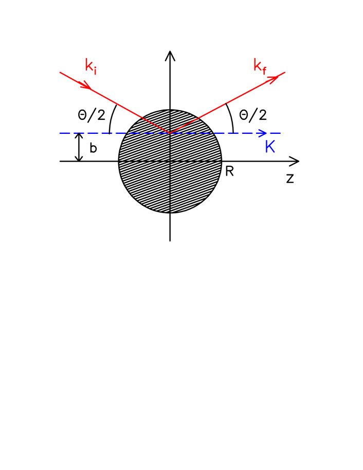
Figure 1: (Color online). Scattering geometry for a potential of radius $R$ showing the impact parameter $b$, the ray made by the incoming and outgoing momenta $\>{\bf k}_{i,f}\>$, and the mean momentum ${\bf K}=({\bf k}_{i}+{\bf k}_{f})/2$.

What happens for a nonlocal potential $\hat{V}$? In this case we have to start not from the Lagrangian path integral (2) but from the more general phase-space path integral

$$U({\bf x}_{b},T;{\bf x}_{a},-T) = \int_{{\bf x}(-T)={\bf x}_{a}}^{{\bf x}(T)={\bf x}_{b}}{\cal D}^{3}x(t)\,\int{\cal D}^{3}p(t)$$ (17)

$$\times\,\exp\Biggl{\{}\,i\int_{-T}^{+T}dt\Bigl{[}{\bf p}(t)\cdot\dot{\bf x}(t)-\frac{{\bf p}^{2}(t)}{2m}$$

$$\hskip 28.45274pt-V_{W}({\bf x}(t),{\bf p}(t))\Bigr{]}\,\Biggr{\}}\>.$$

Here

$$V_{W}({\bf x},{\bf p})\>=\>\int d^{3}y\>\left<{\bf x}-\frac{y}{2}|\hat{V}|{\bf x}+\frac{y}{2}\right>\,e^{i{\bf p}\cdot{\bf y}}$$ (18)

is the Wigner transform of the quantum-mechanical operator $\hat{V}$. Using it in the phase-space path integral is equivalent to applying Weyl’s quantization rule to velocity-dependent interactions (the “mid-point” rule). One can now follow all the previous steps to derive a path-integral representation of the $T$-matrix. Writing the additional (unconstrained) momentum variable ${\bf p}(t)=m\,{\bf u}(t)$ and using a 3-dimensional antivelocity we then arrive at the following expression

$${\cal T}_{i\to f}^{(3-3)} = i\frac{K}{m}\>\int d^{2}b\>e^{-i{\bf q}\cdot{\bf b}}\>\int{\cal D}^{3}v\,{\cal D}^{3}w\,{\cal D}^{3}u$$ (19)

$$\times\exp\left\{\,i\,\int\limits_{-\infty}^{+\infty}dt\,\frac{m}{2}\,\biggl{[}\,{\bf v}^{2}(t)-{\bf w}^{2}(t)-{\bf u}^{2}(t)\,\biggr{]}\,\right\}$$

$$\times\Bigl{\{}\>\exp\left[\>i\,\chi({\bf b},{\bf v},{\bf w},{\bf u})\>\right]-1\>\Bigr{\}}$$

where the phase function(al) is now

$$\chi({\bf b},{\bf v},{\bf w},{\bf u})=-\!\int\limits_{-\infty}^{+\infty}dt\,V_{W}\bigl{[}\mbox{\boldmath$\xi$}(t),{\bf K}+m{\bf v}(t)+m{\bf u}(t)\bigr{]}$$ (20)

and $\mbox{\boldmath$\xi$}(t)$ has been defined in Eq. (13). Again the path integrals are normalized such that Gaussian integrals are unity as in Eq. (7).

3 Applications

3.1 Eikonal expansions

For high-energy and small scattering angles the particle mainly travels along the reference path as shown by an appropriate scaling of variables Rose : all quantum fluctuations are suppressed by inverse powers of $K=k\cos(\theta/2)$ for the representation with a 3-dimensional antivelocity and by inverse powers of $k$ for the “ray” version. In the former case the leading term is given by

$${\cal T}_{i\to f}\!\simeq\!\frac{iK}{m}\!\int\!\!d^{2}be^{-i{\bf q}\cdot{\bf b}}\Biggl{\{}\exp\left[-i\int\limits_{-\infty}^{+\infty}\!dtV\left({\bf b}+\frac{{\bf K}t}{m}\right)\right]-1\Biggr{\}},$$ (21)

a version of the eikonal approximation due to Abarbanel and Itzykson AI . Higher-order corrections can be calculated systematically and agree with the systematic eikonal expansion due to Wallace Wal . In the nonlocal case neglecting all quantum fluctuations ${\bf v}(t),{\bf w}(t),{\bf u}(t)$ in Eq. (19) gives an approximation for the $T$-matrix first derived in Ref. Rowig .

3.2 Variational approximations

The new path-integral representations for the $T$-matrix suggest new variational approximations by applying the Feynman-Jensen variational principle. This has been studied in Ref. Carr with a trial action which is linear in the velocities ${\bf v}(t),{\bf w}(t)$ and in Ref. CaRo with a more general (linear + quadratic) trial action. In both cases the first correction to the variational result from a cumulant expansion has also been evaluated and impressive agreement with partial-wave calculations has been found, even for larger scattering angles.

3.3 Stochastic evaluation of high-energy scattering

One may try to evaluate the path integral for the $T$-matrix numerically by stochastic methods as is done in the Euclidean case. For this purpose (and for simplicity in the representation with a 3-dimensional antivelocity) we expand the velocity variables in a complete set of harmonic oscillator functions

$$\left(\begin{array}[]{c}{\bf v}(t)\\ {\bf w}(t)\end{array}\right)\>=\>C\,\sum_{n=0}^{\infty}\,\left(\begin{array}[]{c}{\bf v}_{n}\\ {\bf w}_{n}\end{array}\right)\,u_{n}\left(\frac{t}{t_{0}}\right)\>.$$ (22)

Here $t_{0}$ denotes a characteristic time which we take as the one needed to traverse the range $R$ of the potential, i. e. $t_{0}=mR/k$ and the constant $C$ is chosen such that the free action becomes

$$S_{0}\>=\>\sum_{n=0}^{\infty}\left({\bf v}_{n}^{2}-{\bf w}_{n}^{2}\right)\>.$$ (23)

Writing

$$\mbox{\boldmath$\xi$}(t)\>=\>{\bf b}+\frac{{\bf K}}{m}t+{\bf x}_{\rm quant}(t)$$ (24)

the quantum trajectory is then given by

$${\bf x}_{\rm quant}(t)\>=\>\sum_{n=0}^{\infty}\left[\,q_{n}\left(\frac{t}{t_{0}}\right)\>{\bf v}_{n}-q_{n}(0)\,{\bf w}_{n}\,\right]$$ (25)

where

$$q_{n}(y)\>:=\>\frac{Ct_{0}}{2}\,\int_{-\infty}^{+\infty}dx\>{\rm sgn}(y-x)\,u_{n}(x)\>.$$ (26)

Completeness of the harmonic-oscillator wave functions implies

$$\sum_{n=0}^{\infty}q_{n}\,\left(\frac{t_{1}}{t_{0}}\right)q_{n}\left(\frac{t_{2}}{t_{0}}\right)\>=\>\frac{1}{m}\,\Bigl{[}\,T-\left|t_{1}-t_{2}\right|\,\Bigr{]}$$ (27)

where the divergence of the infinite sum has been regulated by a large scattering time $T$ as before.

The path integral (12) can now be written as an infinite-dimensional integral over the expansion coefficients

$${\cal T}_{i\to f}^{(3-3)}\! = \!\frac{iK}{m}\int\!d^{2}b\,e^{-i{\bf q}\cdot{\bf b}}\,\left\{\prod_{n=0}^{\infty}\!\left(\int d^{3}v_{n}d^{3}w_{n}\right)\,e^{iS_{0}}\right\}^{-1}$$ (28)

$$\quad\times\prod_{n=0}^{\infty}\left(\int d^{3}v_{n}\,d^{3}w_{n}\right)\>e^{iS_{0}}\,\Bigl{(}e^{i\chi}\,-\,1\>\Bigr{)}\>.$$

In any numerical calculation the infinite sum over the modes $n$ has to be reduced to a finite one involving only $N$ modes. Therefore we split the free action into two parts , one ($S_{0}^{<}$) involving the lower modes $n=0,\,\ldots N-1$ and the other ($S_{0}^{>}$) depending only on the “upper” expansion coefficients $n=N,\,\ldots\infty$.

For the upper modes we employ the method of “partial averaging” PA , i. e.

$$\left<\,e^{i\chi}\,\right>_{N}^{\infty}\> := \frac{\prod_{N}^{\infty}\left(\int d^{3}v_{n}d^{3}w_{n}\right)\>\exp\left(\,iS_{0}^{>}\,\right)\>e^{i\chi}}{\prod_{N}^{\infty}\left(\int d^{3}v_{n}d^{3}w_{n}\right)\>\exp\left(\,iS_{0}^{>}\,\right)}$$ (29)

$$\simeq \exp\left(\>i\left<\,\chi\,\right>_{N}^{\infty}\>\right)\>.$$

In Fourier path integrals partial averaging has been successfully applied to determine the ground-state and thermal properties of bound systems (see, e.g. Ref. AlRo ). It includes the upper modes (up to infinity) at least approximately by averaging them with the free action thereby improving convergence with the number $N$ of explicit modes KFD .

Here we apply this method to a scattering problem. Note that $\left<\chi\right>_{N}^{\infty}$ depends on the lower coefficients and acts as a (complex) interaction phase for the $6N$-dimensional integral over the coefficients ${\bf v}_{n},{\bf w}_{n},\>n=0,\,\ldots N-1$. The free average of the potential over the upper coefficients is readily performed as only Gaussian integrals have to be evaluated and one obtains

$$\left<\chi\right>_{N}^{\infty}\>=\>-\int_{-\infty}^{+\infty}dt\>V_{\sigma(t)}\left({\bf x}_{\rm quant}^{<}(t)\right)$$ (30)

where

$${\bf x}_{\rm quant}^{<}(t)\>:=\>\sum_{n=0}^{N-1}\left[\,q_{n}\left(\frac{t}{t_{0}}\right)\,{\bf v}_{n}-q_{n}(0)\,{\bf w}_{n}\,\right]$$ (31)

is the quantum trajectory involving the lower coefficients and

$$\tilde{V}_{\sigma(t)}({\bf p})\>:=\>\tilde{V}({\bf p})\,\exp\left[\,-\frac{1}{2}\,\sigma(t){\bf p}^{2}\,\right]\>,$$ (32)

the Gaussian transform of the potential in momentum space. The width turns out to be purely imaginary

$$\sigma_{N}(t/t_{0})\>:=\>\frac{i}{2}\sum_{n=N}^{\infty}\left[\,q_{n}^{2}\left(\frac{t}{t_{0}}\right)-q_{n}^{2}(0)\,\right]$$ (33)

where the first term in the bracket comes from the velocity integration and the last one from the integration over the antivelocity. Due to Eq. (27) we can write it as

$$\sigma_{N}(t/t_{0})\>=\>\frac{i}{2m}\left[\,T-T\,\right]+\frac{i}{2}\sum_{n=0}^{N-1}\left[\,q_{n}^{2}(0)-\,q_{n}^{2}\left(\frac{t}{t_{0}}\right)\,\right]$$ (34)

showing how the arising divergence is exactly cancelled by the contribution of the antivelocity.

Still it is impossible to evaluate the remaining $6N$-dimensional integral over the lower coefficients without any damping. This is provided by giving the particle a complex mass

$$m_{\rm particle}\>\longrightarrow\>m\,\left(1+i\Gamma\right)$$ (35)

and the phantom the mass $m^{\star}$

$$m_{\rm phantom}\longrightarrow m\,\left(1-i\Gamma\right)\>.$$ (36)

If this is done in the full path integral, $\Gamma\to\infty$ would lead to the eikonal approximation because all quantum fluctuations are suppressed in that limit and $\Gamma\to 0$ would give the exact result. This supports the hope that numerical evaluations at finite $\Gamma$ and an extrapolation of these results to $\Gamma\to 0$ would yield reasonably accurate results for the $T$-matrix.

However, it is not possible to modify the path integral over the upper coefficients in this way as the phantom must have the same mass as the particle: If it would have a different mass, say $\lambda m$ then the second term on the r.h.s of Eq. (34) would be multiplied by $1/\lambda$ and the diverging term $T$ (originating from the particle) would not be cancelled. So partial averaging and damping do not marry (easily) …

If they remain separated, i. e. if only the explicit modes are damped then the stochastic results only slowly converge to the exact ones if $\Gamma$ is decreased. This is shown in Fig. 2 where scattering from a Gaussian potential

$$V(r)\>=\>V_{0}\,e^{-r^{2}/R^{2}}$$ (37)

at a fixed scattering angle is considered for $N=1$. It is seen that the relative deviation of the stochastic scattering amplitude indeed decreases if the damping is made smaller but that one also needs more and more Monte-Carlo calls to obtain a statistically valid result.

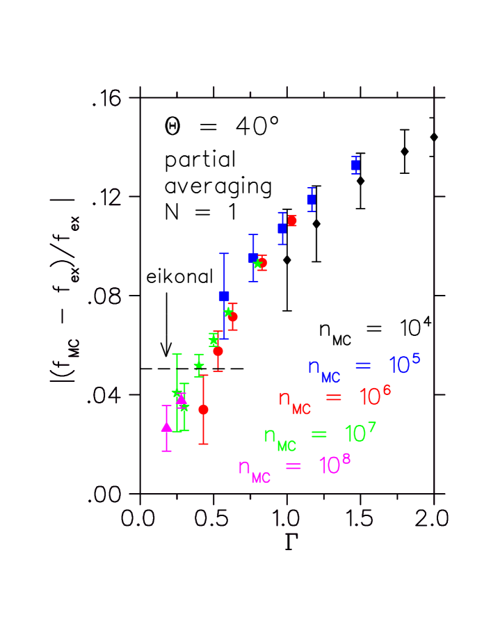
Figure 2: (Color online). The relative deviation $|\Delta f/f|$ of the stochastic scattering amplitude from the exact partial wave result at a fixed scattering angle $\theta=40^{o}$ for scattering from the Gaussian potential (37) with $2mV_{0}R^{2}=-4$ at $kR=4$.

Although encouraging these results indicate that further work is needed to obtain a practical Monte-Carlo scheme for high-energy potential scattering. For a different approach see Ref. Smir .

4 Relativistic extensions

To stay closer to the spirit and the aims of this workshop I will now consider scattering under relativistic conditions, i.e. truly high-energy scattering. In my opinion quantum field theory provides the most general, consistent - albeit not the most practical - framework to describe these phenomena and therefore I will consider a scalar theory of particles ($\Phi$) with mass $M$ interacting by exchange of scalar particles ($\phi$) of mass $m$ given by an interaction Lagrangian

$${\cal L}_{I}\>=\>g\,\left|\Phi^{2}\right|\,\phi\>.$$ (38)

This generalized Wick-Cutkosky model Wick ; Cut mimics meson-exchange between massive nucleons and – 55 years after its introduction – is still the favorite model  of many workers in the field mostly for the relativistic bound-state problem (see, e.g. Ref. BRS ).

Let us evaluate the 4-point function of the theory: neglecting nucleon loops (“quenched approximation”) and using the Schwinger representation for the nucleon propagator in the presence of the meson field

$$\left[-\partial^{2}-M^{2}+g\,\phi(x)+i0\right]^{-1}\>=\>$$

$$\quad\frac{1}{iM}\int_{0}^{\infty}dT\>\exp\left[\frac{i}{M}\left(-\partial^{2}-M^{2}+g\,\phi(x)\right)T\right]$$ (39)

the 4-point function for scattering of two nucleons can be written in “worldline” form

$$G_{4}(x_{1},x_{2},x_{3},x_{4})=\int_{0}^{\infty}\!\!dT_{1}\,dT_{2}\,\exp\left[-iM\left(T_{1}+T_{2}\right)\right]$$

$$\times\,\int_{y_{1}(-T_{1})=x_{1}}^{y_{1}(+T_{1})=x_{2}}{\cal D}^{4}y_{1}\int_{y_{2}(-T_{2})=x_{3}}^{y_{2}(+T_{2})=x_{4}}{\cal D}^{4}y_{2}$$

$$\times\exp\Biggl{(}\,iS_{0}[y_{1},y_{2}]+iS_{\rm int}[y_{1},y_{2}]\,\Biggr{)}+\left(\,x_{1}\leftrightarrow x_{3}\,\right).$$ (40)

Here the free action is given by

$$S_{0}[y_{1},y_{2}]\>=\>\sum_{i=1}^{2}\int_{-T_{i}}^{+T_{i}}d\tau\left(-\frac{M}{2}\dot{y}_{i}^{2}\right)$$ (41)

while the interaction part is retarded because the mesons have been integrated out:

$$S_{\rm int}[y_{1},y_{2}] = -\frac{g^{2}}{8M^{2}}\sum_{i,j=1}^{2}\int_{-T_{i}}^{+T_{i}}d\tau_{1}\int_{-T_{j}}^{+T_{j}}d\tau_{2}\>\int\frac{d^{4}p}{(2\pi)^{4}}$$ (42)

$$\times\frac{1}{p^{2}-m^{2}+i0}\,\exp\left[\,-ip\cdot\left(y_{i}(\tau_{1})-y_{j}(\tau_{2})\right)\right]\>.$$

This looks (superficially) very similar to a nonrelativistic description: if we neglect the $(i=j)$-terms, i. e. the self-energy of the nucleons, then we have a 4-dimensional analogue of scattering from a Yukawa potential. Still there are two different proper times $T_{1},T_{2}$ over which one has to integrate finally and a mass renormalization is needed to get rid of the divergencies at small proper time – of course, all these features are to be expected in a relativistic quantum field theory .

To obtain the relativistic $T$-matrix one has to Fourier transform the 4-point function (40) (easily done by converting to velocity path integrals), extract the energy-momentum-conserving $\delta$-function and remove the outer legs, i.e. multiply with the inverse (full) 2-point functions of the external particles. While the extraction of energy-momentum conservation is obvious in this field-theoretic framework due to the translation invariance of the action, the amputation of the full external nucleon propagators is more involved. Using the Bloch-Nordsieck approximation it is possible to achieve that by functional differentiation techniques (see, e.g. Ch. 10.1 in Ref. Fried ) but I expect that introducing phantom degrees of freedom as in the nonrelativistic case will do a better job. This is presently under investigation.

5 Summary

Several path integral representations for the $T$-matrix in potential scattering have been discussed, including a new one for nonlocal potentials. They serve to derive high-energy expansions, variational approximations and are a natural starting point for a stochastic evaluation of high-energy potential scattering. Many avenues lie open for further development, in particular in the relativistic domain.

Note added after publication:   A method for non-perturbative amputation of the 4-point function in the Wick-Cutkosky model and in scalar QED has been developed by Barbashov and collaborators Barb1 ; Barb2 ; MaTa . See also Refs. HaXu ; HaPo .

References

• (1) Koch, J., Mall, H., Lenz, S.: Stochastic methods for zero energy quantum scattering. Comp. Phys. Comm. 108, 115 (1998)
• (2) Rosenfelder, R.: Path integrals for potential scattering. Phys. Rev. A 79, 012701 (2009)
• (3) Lee, T. D., Wick, G. C.: Negative metric and the unitarity of the S-matrix. Nucl. Phys. B 9, 209 (1969)
• (4) Grinstein, B., Oโ€™Connell, D., Wise,M. B.: The Lee-Wick standard model. Phys. Rev. D 77, 025012 (2008)
• (5) Abarbanel, H. D. I., Itzykson, C.: Relativistic eikonal expansion. Phys.ย Rev.ย Lett.ย  23, 53 (1969)
• (6) Wallace, S. J.: Eikonal expansion. Ann. Phys.ย  78, 190 (1973)
• (7) Rosenfelder, R.: Wigner transform and the eikonal approximation for nonlocal potentials. Z. Phys. A 293, 25 (1979)
• (8) Carron, J.: Variational methods for path integral scattering. arXiv:0903.0273 [nucl-th]
• (9) Carron, J., Rosenfelder, R.: Variational approximations in a path-integral description of potential scattering. Eur. Phys. J. A 45, 193 (2010)
• (10) Doll, J. D., Coalson, R. D., Freeman, D.L.: Fourier path-integral Monte Carlo methods: Partial averaging. Phys.ย Rev.ย Lett.ย  55, 1 (1985)
• (11) Alexandrou, C., Rosenfelder, R.: Stochastic solution to highly nonlocal actions: The polaron problem. Phys.ย Rept.ย  215, 1 (1992)
• (12) Kunikeev, S. D., Freeman, D. L., Doll, J. D.: Convergence characteristics of the cumulant expansion for Fourier path integrals. arXiv:1006.1641v1 [physics.comp-ph]
• (13) Johnson, G. W., Lapidus, M. L.: The Feynman integral and Feynmansโ€™s operational calculus, 771 p. Oxford University Press, Oxford (2000)
• (14) Smirnov, V. V.: Test of a path-integral approach for the computation of scattering cross sections on an exactly solvable model. Phys. Rev. A 76, 052706 (2007)
• (15) Wick, G. C.: Properties of Bethe-Salpeter wave functions. Phys.Rev.96, 1124 (1954)
• (16) Cutkosky, R. E.: Solutions of a Bethe-Salpeter equation. Phys.ย Rev.ย  96, 1135 (1954)
• (17) Baym, G.: Inconsistency of cubic boson-boson interactions- Phys.ย Rev.ย  117, 886 (1960)
• (18) Barro-Bergflรถdt, K., Rosenfelder, R., Stingl, M.: Variational worldline approximation for the relativistic two-body bound state in a scalar model. Few Body Syst.ย  39, 193 (2006)
• (19) Fried, H. M.: Basics of functional methods and eikonal models, 326 p. Editions Frontiรจres, Gif-sur-Yvette, France (1990)
• (20) Barbashov, B. M., Kuleshov, S. P., Matveev, V. A., Sisakyan, A. N.: Eikonal approximation in quantum-field theory. Teor. Mat. Fiz. 3, 342 (1970) [English transl.: Theor. Math. Phys. 3, 555 (1970)]
• (21) Barbashov, B. M., Kuleshov, S. P., Matveev, Pervushin, V. P., Sisakyan, A. N., Tavkhelidze, A. N.: Straight-line paths approximation for studying high-energy elastic and inelastic hadron collisions in quantum field theory. Phys.ย Lett.ย  B 33, 484 (1970)
• (22) Matveev, V. A., Tavkhelidze, A. N.: On the representation of scattering amplitudes as path integrals in quantum field theory. Teor. Mat. Fiz. 9, 44 (1971) [English transl.: Theor. Math. Phys. 9, 968 (1971)]
• (23) Han, N. S., Xuan, N. N.: Planckian scattering beyond the eikonal approximation in the functional approach. Eur.ย Phys.ย J.ย  C 24, 643 (2002) [arXiv:gr-qc/0203054].
• (24) Han, N. S., Ponna, E.: Straight-line path approximation for studying Planckian-energy scattering in quantum gravity. Nuov. Cim A A 110, 459 (1997)