Parameter-free dissipation in simulated sliding friction

Abstract

Non-equilibrium molecular dynamics simulations, of crucial importance in sliding friction, are hampered by arbitrariness and uncertainties in the way Joule heat is removed. We implement in a realistic frictional simulation a parameter-free, non-markovian, stochastic dynamics, which, as expected from theory, absorbs Joule heat precisely as a semi-infinite harmonic substrate would. Simulating stick-slip friction of a slider over a 2D Lennard-Jones solid, we compare our virtually exact frictional results with approximate ones from commonly adopted empirical dissipation schemes. While the latter are generally in serious error, we show that the exact results can be closely reproduced by a viscous Langevin dissipation at the boundary layer, once the back-reflected frictional energy is variationally optimized.

The role of Molecular Dynamics (MD) simulation in the theory of sliding friction and nanofriction can hardly be overestimated Persson (1998); Robbins and Müser (2001). In a typical simulation, a slider is driven by an external force over a simulated solid substrate whose atoms, interacting through realistically chosen interatomic forces, vibrate and move according to Newton’s law. Naturally, in order to attain a frictional steady state the Joule heat must be removed. Unfortunately, a realistic energy dissipation is generally impossible to simulate reliably, owing to size (and time) limitations. In a small size simulation cell, the phonons generated at the sliding interface are back-reflected by the cell boundaries, rather than propagated away to properly disperse the Joule heat. The ensuing problem is a spuriously accumulating phonon population in the slider-substrate interface region. The empirical introduction in the equations of motion of ad-hoc Langevin viscous damping terms $-m\gamma_{i}\dot{q}_{i}$ (with $m$ and $\dot{q}_{i}$ the mass and the velocity of the $i$-th particle) and of an associated random noise, corresponding to some “thermostat” temperature $T$ Zwanzig (2001), represents the handiest and commonest solution. However, both this procedure and the choice of thermostat and damping parameters $\gamma_{i}$ are vastly arbitrary. The problem is not just one of principle. Dry friction generally involves stick-slip Persson (1998), and each slip generates a burst of phonons of very specific nature and composition. In realistic simulations the overall effect on frictional dynamics of the partial back-reflection of this burst must be minimized. Unless dealt with, back-reflection will cause the simulated steady state and friction coefficient to depend upon unphysical damping parameters. In the Prandtl-Tomlinson model Vanossi and Braun (2007) for instance, damping is known to modify the kinetics and the friction, both in the stick-slip regime (including the multiple-slips seen in Atomic Force Microscopy Medyanik et al. (2006)) and in the smooth sliding state. To a lesser or larger extent this lamentable state of affairs is common to all MD frictional simulations.

Pursuing a viable solution, one wishes to modify the equations of motion inside a relatively small simulation cell, so that they will reproduce the frictional dynamics of a much larger system, once the remaining variables are integrated out. Integrating out degrees of freedom is a classic problem, largely analysed in literature Rubin (1960); Zwanzig (2001); Li and E (2007); Kantorovich (2008); Kantorovich and Rompotis (2008). In the context of MD simulation, Green’s function methods were formulated for quasistatic mechanical contacts Campana and Müser (2006); approaches based on a discrete-continuum matching have also been discussed Luan et al. (2006); E and Huang (2001).

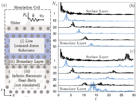
Figure 1: (Color online) (a) Sketch of the simulated system. (b),(c) Layer-averaged kinetic energy time evolution of a surface-injected phonon burst. Phonon back-reflection is strong without dissipation at the boundary layer (c), but accurately canceled once the correct dissipative kernels are included (b).

Among others, a formally exact dissipation formulation was given early on by Rubin Rubin (1960). Integrating out $N-1$ atoms in a linear harmonic chain yields a non-markovian Langevin-like equation of motion of a single atom of interest. Extensions of this method were applied to a variety of problems, including the relaxation of impurity molecules in solids Shugard et al. (1978); Nitzan et al. (1978), and atom-surface scattering Adelman and Doll (1976, 1974). Detailed formulations suitable for MD simulations were given by Li et al. Li and E (2007) and by Kantorovich Kantorovich (2008); Kantorovich and Rompotis (2008); Toton1 et al. (2010). The idea to variationally minimize back-reflection of individual phonons has also been put forward Li and E (2007). However, this body of theory has not yet found its way into realistic sliding friction MD simulations, so that neither the importance of back-reflection errors in dry friction, nor a realistic way to get rid of them have really been demonstrated. Here we describe how both goals are achieved, in a simulated 2D Lennard-Jones system that exhibits a realistic stick-slip. We find that exact stick-slip friction is indeed different from that of empirical damping schemes. However the back-reflected energy can be variationally minimized – although differently from Li et al. — the resulting approximate dynamics now reproducing quite accurately the exact benchmark stick-slip friction.

We focus on a model sliding system made of a semi-infinite two-dimensional crystalline substrate with $N_{z}$ monatomic layers each of $N_{x}$ atoms, and of a slider made of a single chain of $N^{\prime}_{x}$ atoms. All atoms interact via a Lennard-Jones (LJ) potential (cutoff for simplicity to first-neighbors). The slider is pressed against the substrate by a normal “load” force $F_{0}$, and is driven along $x$ (parallel to the substrate) through a spring of strength $k$, whose end is pulled at constant velocity $v_{0}$. Following similar earlier formulations Li and E (2007); Kantorovich (2008); Kantorovich and Rompotis (2008), the ideal infinitely thick substrate is divided as in Fig. 1(a), into three regions: (i) a live slab comprising $N_{z}-1$ atomic layers whose motion is fully simulated by Newton’s equations; (ii) the dissipative boundary ($N_{z}$-th) layer, whose motion includes the effective non-markovian Langevin terms; (iii) the remaining semi-infinite solid acting as a phonon absorber, or heat bath, whose degrees of freedom are integrated out, providing the source of effective damping terms in (ii). In our practical implementation we substitute the full LJ potential within region (iii) and between (ii) and (iii) with its harmonic approximation. This approximation, necessary in order to get an analytical form for the effective forces on the boundary atoms, is all the more accurate the weaker the intensity of frictional phonons. In practice, for crystal substrates above quantum freezing and below the Debye temperature, this level of accuracy can always be attained by a sufficient thickness $N_{z}-1$ of the live simulation cell (i). The harmonic heat bath (iii) is decoupled by diagonalizing the dynamical matrix $D_{\mu\nu}^{kl}$ ($k,l$ denoting atoms), obtaining eigenvalues $\omega^{2}_{k}$ and eigenvectors $\boldsymbol{\lambda}_{k}$. The equations of motion for the boundary layer atoms are Li and E (2007); Kantorovich (2008)

$$m\ddot{q}^{i}_{\mu}(t) = -\frac{\partial U_{sub}}{\partial q^{i}_{\mu}}-m\sum_{j,\nu}\int_{0}^{t}\!ds\;K^{ij}_{\mu\nu}(t-s)\;\dot{q}^{j}_{\nu}(s)$$ (1)

$$+R^{i}_{\mu}(t)+\sum_{j,\nu}q^{j}_{\nu}(t)\bigg{(}K^{ij}_{\mu\nu}(0)-D^{ij}_{\mu\nu}\bigg{)}\;,$$

where $i$ and $j$ denote boundary layer atoms, $\mu$ and $\nu$ indicate $x/z$ components, $U_{sub}$ is the LJ interaction between the $i$-th boundary atom and those inside the simulation cell (i). The second term is non-markovian and non-conservative, introducing an effective damping proportional to the velocity of the $j$-th atom, through a time convolution with the memory kernel functions $K^{ij}_{\mu\nu}(t)$. Standard kernels are built from the harmonic eigenvalues and eigenvectors of the heat-bath dynamical matrix and from the coupling vectors $\boldsymbol{\phi}_{\mu}^{i}$ containing the harmonic coupling constants $D_{\mu\mu}^{ik}$ and $D_{\mu\nu}^{ik}$ of the $i$-th atom of region (ii) with the $k$-th heat-bath atom $K^{ij}_{\mu\nu}(t)=\sum_{k}\bigg{[}\frac{(\boldsymbol{\lambda}_{k}\cdot\boldsymbol{\phi}_{\mu}^{i})(\boldsymbol{\phi}_{\nu}^{j}\cdot\boldsymbol{\lambda}_{k})}{\omega^{2}_{k}}\bigg{]}\;\cos{(\omega_{k}t)}$. They oscillate and decay with time, with power law tails due to the bath acoustical phonon branches. Periodic boundary conditions along the $x$ direction guarantee translational invariance, so that $K^{ij}_{\mu\nu}(t)$ is a function of $|i-j|$ only. As kernels inherit their symmetry properties from those of the heat-bath dynamical matrix, one can show that $K^{ij}_{\mu\nu}(t)=-K^{ij}_{\nu\mu}(t)$ and $K^{ij}_{\mu\nu}(t)=K^{ji}_{\nu\mu}(t)$. As $|i-j|$ grows, $|K^{ij}_{\mu\nu}(t)|$ decrease, but again not exponentially, so that correlations must be included up to large distance Li and E (2007). By cutting kernels off at time $\tau_{c}$ one could limit the time-integrals in Eq. (1), which need to be calculated at each time step. By increasing both $\tau_{c}$ and the live simulation cell size $N_{z}$, one refines the dissipation scheme accuracy as much as desired, although at increased computational cost. The third term in Eq. (1) is a gaussian stochastic force present at non-zero temperature, responsible for the energy transfer between the heat-bath (iii) and the live substrate (i), with $\langle R^{i}_{\mu}(t)\rangle=0$, and $\langle R^{i}_{\mu}(t)R^{j}_{\nu}(t^{\prime})\rangle=mk_{B}TK^{ij}_{\mu\nu}(t-t^{\prime})$ where brackets denote ensemble average, $k_{B}$ is Boltzmann’s constant and $T$ the temperature. As is well known Zwanzig (2001), this relationship fulfils the fluctuation-dissipation theorem — the scheme represents a well defined thermostat in contact with the simulation cell. The last term in Eq. (1) is the harmonic coupling between atoms $i$-th and $j$-th within the boundary layer, where the coupling constant $D_{\mu\nu}^{ij}$ is modified by $K^{ij}_{\mu\nu}(0)$.

As a first step before simulating friction we implement the set of equations (1), along with ordinary Newton’s equations governing the live cell in an MD simulation, to test phonon reflection. Starting with the equilibrated system ($N_{z}=30$ close packed layers and $N_{x}=10$ atoms per layer) at temperature $T$, a test burst of phonons is introduced at the topmost layer and time-evolved. Results in Fig. 1(b) show how a relatively thin $N_{z}=30$ layer substrate (i+ii) is able to mimick, within the exact dissipation scheme, the full ideal semi-infinite system (i+ii+iii). Layer-resolved kinetic energies inside the simulated substrate show the group of phonons propagating below the surface. Upon reaching the boundary layer the phonons are perfectly absorbed as if they propagated into the (integrated out) semi-infinite crystal (iii). For comparison, Fig. 1(c) shows the same phonons massively back reflected once the memory kernels are removed from the boundary layer.

We next simulate stick-slip sliding friction by driving a slider, here consisting of a LJ chain of $N^{\prime}_{x}=9$ atoms, over the same live substrate as above  . The instantaneous friction force is measured by the spring elongation $F(t)=k(x_{CM}-v_{0}t)$, $x_{CM}$ being the slider center of mass position. The sawtooth force profile typical of stick-slip friction is obtained (Fig. 2 (a)). The friction coefficient, obtained by averaging over a stationary sequence of stick-slips is $\langle F\rangle/F_{0}=0.116\pm 0.002$. The stick-slip pattern is irregular, with a periodicity similar but not exactly matching, a substrate lattice spacing. The highest spikes signal the forward jump of most slider atoms, smaller ones involve only about $2/3$ of them. A measure of the distribution of the spike heights is the variance of $F(t)$, i.e., $\sigma=\frac{1}{\tau_{s}\langle F\rangle^{2}}\int_{0}^{\tau_{s}}[F(t)-\langle F\rangle]^{2}dt$, where $\tau_{s}$ is the total simulation time. These simulations using the full Eq. (1), and the corresponding frictional results can be considered essentially exact, and represent our benchmark reference of stick-slip friction with a correct Joule heat removal. The numerical implementation of this standard scheme in a generic 3D case will in principle be possible but time consuming, and far from handy. Long-range non-markovian correlations imply a general scaling as $N_{x}^{2}$, so that simulations for large-size 3D sliding systems may pose a

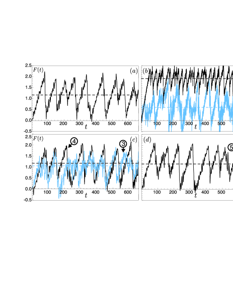
Figure 2: (Color online) (a) Simulated friction force $F(t)$ for the “exact” non-markovian dissipation scheme of Eq. (1), and [(b),(c) and (d)] for empirical Langevin schemes with a $-\gamma\dot{q}$ damping applied to tip L1, whole substrate L2 and bottom layer L3. The $\gamma$ value is identified by numbers $1$-$5$ in Fig.3. Dashed lines: mean value $\langle F\rangle$.

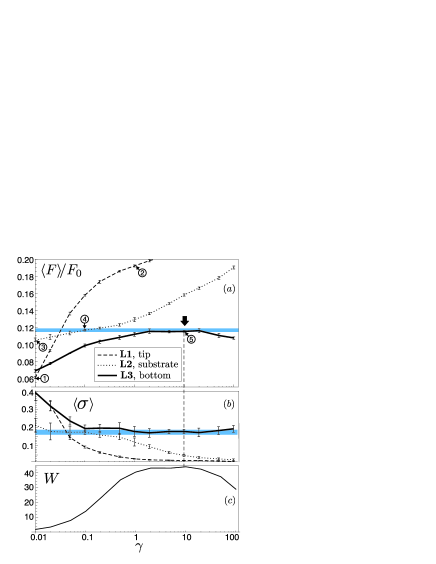
Figure 3: (Color online) (a),(b) Friction coefficient $\langle F\rangle/F_{0}$ and variance $\langle\sigma\rangle$ as a function of a viscous damping $\gamma$ for different empirical Langevin dissipation schemes, compared with exact non-markovian values (blue stripes). (c) Average internal energy $W$ per substrate atom for the markovian thermostat L3 divided by the internal energy $W_{exact}$ per substrate atom for the non-markovian scheme (1). The exact and empirical frictional behaviour nearly coincide when the boundary layer parameter $\gamma$ is such as to variationally minimize the relative total back-reflected energy $W/W_{exact}$.

practical challenge of parallel computing.

The virtually exact frictional dynamics just obtained can now be compared with empirical Langevin schemes commonly adopted in friction simulations, where a viscous damping $-\gamma\dot{q}$ is arbitrarily applied to the motion of some atoms in the system, for instance to slider atoms (L1, dashed line in Fig.3) or to all substrate atoms (L2, dotted line), or to the boundary atomic layer only (L3, solid line). As anticipated, the stick-slip friction simulated with all these empirical schemes depends vastly on $\gamma$, and generally deviates systematically from the correct benchmark. The closest agreement is obtained in case L3 where the viscous damping $-m\gamma\dot{q}^{i}_{\mu}(t)$ is applied to the $i$-th boundary layer atom motion, $m\ddot{q}^{i}_{\mu}(t)=-\frac{\partial U}{\partial q^{i}_{\mu}}-m\gamma\dot{q}^{i}_{\mu}(t)+R^{i}_{\mu}(t)$, with the appropriate gaussian stochastic force $R_{i}(t)$ with $\langle R^{i}_{\mu}(t)\rangle=0$ and $\langle R^{i}_{\mu}(t)R^{j}_{\nu}(t^{\prime})\rangle=2mk_{B}T\gamma\delta_{\mu,\nu}\delta_{i,j}\delta(t-t^{\prime})$. Since the parameter $\gamma$ is adjustable, we may seek to optimize it in order to approximate the exact results. Li et al.  Li and E (2007) considered variationally minimizing a group-velocity weighted phonon reflection. In the actual friction simulation, the steady state internal energy increase $W=\langle E\rangle-\langle E_{0}\rangle$ over the equilibrium value $E_{0}$ is easily computable. Our proposed scheme is to variationally minimize $W$, a quantity generally positive and proportional to the Joule frictional heat. In absence of back-reflection $W$ is minimal, whereas partial energy reflection at the boundary will cause Joule heat to artificially accumulate in the slab and increase $W$, so that for any arbitrary dissipation scheme $W/W_{exact}>1$. As a function of $\gamma$, a variational minimum of $W/W_{exact}$ occurs because back-reflection of frictional phonons is large both when the boundary layer damping $\gamma$ is too small and too large. This ratio is shown in Fig. 3(c). The agreement between the exact frictional results, where no phonons are back reflected, and the variational one at $\gamma=10$ is excellent. (We note incidentally that at the optimal $\gamma$ the friction coefficient also peaks). To confirm the variational result, we changed system parameters, including sliding velocity, and load. The variable load results of Fig. 4 (inset) show that the coincidence of optimal and exact friction is systematic. Fig. 4 also shows a dependence of calculated friction upon the thickness of the simulated substrate portion (i+ii), converging for sufficiently large $N_{z}$. The required thickness of a few tens of layers depends on velocity, and is reached once the substrate inertia grows large enough to stop interfering spuriously with the frictional dynamics.

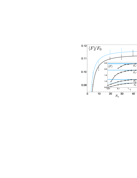
Figure 4: (Color online) Friction coefficient as a function of the simulated cell thickness $N_{z}$ for different driving velocities $v_{0}=0.01$ (blue) and $v_{0}=0.02$ (black) obtained with the non-markovian dissipation scheme. The inset reports the average friction force for different loads $F_{0}$ obtained with the non-markovian approach (blue stripes) and the comparison with the markovian Langevin scheme L3 at different $\gamma$ (black curves).

In conclusion, we demonstrated frictional MD simulations with a nonmarkovian dissipation, enacting the correct disposal of generated phonons, even in the relatively violent stick-slip case. Using the virtually exact frictional results so obtained as a reference, we benchmarked common empirical viscous dissipation schemes, finding them generally wanting. There exists however an optimal viscous damping $\gamma_{opt}$ which, once applied to the cell boundary layer, yields results nearly indistinguishable from the exact ones. The optimal damping parameter variationally minimizes the total back-reflected energy at the cell boundary, and can be identified even without any exact reference calculation. This optimal damping scheme, which unlike the exact one does not require a knowledge of the substrate vibrational properties, is a good candidate for adoption in future practical MD frictional simulations.

A discussion with L. Kantorovich is gratefully acknowledged. This work is part of Eurocores Projects FANAS/AFRI sponsored by the Italian Research Council (CNR), and of FANAS/ACOF. It is also partly sponsored by The Italian Ministry of University and Research, through a PRIN/COFIN contract.

References

- Persson (1998) B. N. J. Persson, Sliding Friction (Springer, Berlin, 1998).
- Robbins and Müser (2001) M. O. Robbins and M. H. Müser, chap. 20 in Modern Tribology Handbook Vol.I (CRC Press, Boca Raton, 2001).
- Zwanzig (2001) R. Zwanzig, Nonequilibrium statistical mechanics (Oxford University Press, New York, 2001).
- Vanossi and Braun (2007) A. Vanossi and O. M. Braun, J. Phys. Cond. Mat. 19, 305017 (2007).
- Medyanik et al. (2006) S. N. Medyanik, W. K. Liu, I.-H. Sung, and R. W. Carpick, Phys. Rev. Lett. 97, 136106 (2006).
- Rubin (1960) R. J. Rubin, J. Math. Phys. 1, 309 (1960).
- Li and E (2007) X. Li and W. E, Phys. Rev. B 76, 104107 (2007).
- Kantorovich (2008) L. Kantorovich, Phys. Rev. B 78, 094304 (2008).
- Kantorovich and Rompotis (2008) L. Kantorovich and N. Rompotis, Phys. Rev. B 78, 094305 (2008).
- Campana and Müser (2006) C. Campana and M. H. Müser, Phys. Rev. B 74, 075420 (2006).
- Luan et al. (2006) B. Q. Luan, S. Hyun, J. F. Molinari, N. Bernstein, and M. O. Robbins, Phys. Rev. E 74, 046710 (2006).
- E and Huang (2001) W. E and Z. Huang, Phys. Rev. Lett. 87, 135501 (2001).
- Shugard et al. (1978) M. Shugard, J. C. Tully, and A. Nitzan, J. Chem. Phys. 69, 336 (1978).
- Nitzan et al. (1978) A. Nitzan, M. Shugard, and J. C. Tully, J. Chem. Phys. 69, 2525 (1978).
- Adelman and Doll (1976) S. A. Adelman and J. D. Doll, J. Chem. Phys. 64, 2375 (1976).
- Adelman and Doll (1974) S. A. Adelman and J. D. Doll, J. Chem. Phys. 61, 4242 (1974).
- Toton1 et al. (2010) D. Toton1, C. Lorenz, N. Rompotis, N. Martsinovich, and L. Kantorovich, J. Phys.: Condens. Matter 22, 074205 (2010).